CLASSIFIER PGN: CLASSIFICATION WITH HIGH CONFIDENCE RULES
Iliya Mitov, Benoit Depaire, Krassimira Ivanova, Koen Vanhoof
Abstract. Associative classifiers use a set of class association rules,
gen-erated from a given training set, to classify new instances. Typically, these techniques set a minimal support to make a first selection of appropriate rules and discriminate subsequently between high and low quality rules by means of a quality measure such as confidence. As a result, the final set of class association rules have a support equal or greater than a predefined threshold, but many of them have confidence levels below 100%. PGN is a novel associative classifier which turns the traditional approach around and uses a confidence level of 100% as a first selection criterion, prior to maxi-mizing the support. This article introduces PGN and evaluates the strength and limitations of PGN empirically. The results are promising and show that PGN is competitive with other well-known classifiers.
1. Introduction. Within the data mining community, research on clas-sification techniques has a long and fruitful history. Clasclas-sification techniques based on association rules, called associative classifiers (AC), are relatively new.
ACM Computing Classification System(1998): H.2.8, H.3.3. Key words: Association rules, classification, high confidence rules.
Associative classifiers generate a set of association rules from a given training set and use these rules to classify new instances. In 1998, Liu et al. [16] in-troduced CBA, often considered to be the first associative classifier. During the last decade, various other associative classifiers were introduced, such as CMAR [15], ARC-AC [4], ARC-BC [4], CPAR [27], CorClass [29], ACRI [22], TFPC [7], HARMONY [25], MCAR [24], 2SARC1 [5], 2SARC2 [5], CACA [23] and ARUBAS [9].
Typically, the generation of association rules from a training set is guided by the support and confidence metrics. Many associative classifiers set a minimum support level and use the confidence metric to rank the remaining association rules. This approach, with a primary focus on support and confidence as the second criterion, will reject 100% confidence rules if the support is too low.
In this article, we question this common approach which prioritizes sup-port over confidence. We study a new associative classifier algorithm, called PGN, which turns the priorities around and focuses on confidence first by retaining only 100% confidence rules. The main goal of this research is to verify the quality of the confidence-first concept. We therefore did not focus on the computational ef-ficiency in this paper, which is left for future research in case the confidence-first concept is supported empirically.
The next section will introduce the related research and positions our approach into the academic literature of associative classification. Next, Section 3 explains the different steps of the PGN algorithm, while Section 4 discusses the results from the empirical analysis of PGN. Finally, conclusions and ideas for future research are stated in Section 5.
2. Associative Classifiers. Associative Classifiers are classification methods which belong to the domain of Data Mining. Fayyad et al. [10] iden-tify Data Mining as the essential step in Knowledge Discovery process where intelligent methods are applied in order to extract data patterns. According to the taxonomy given by Maimon and Rokach [17], data mining methods can be divided into verification methods and discovery methods. Verification methods deal with the evaluation of a hypothesis proposed by an external source, while discovery methods try to identify patterns in data.
Associative Classifiers belong to the family of discovery methods, and more in particular to the predictive discovery methods. Among the predictive discovery methods, one can discern classification and estimation methods. Es-timation methods map the input space onto a real-valued domain and are used when the outcome or predicted variable is continuous. Classification methods, to
which associative classifiers belong, map the input space onto predefined classes and they are used when the outcome or predicted variable is categorical or nom-inal. Other types of classification methods or classifiers are Support Vector Ma-chines [6], Decision Trees [20, 21], k-Nearest-Neighbor classifiers [3] and Neural Networks.
Compared to other classification methods, associative classifiers hold some interesting advantages [28]. Firstly, high dimensional training sets can be han-dled with ease and no assumptions are made about the dependencies between attributes. Secondly, the classification is often very fast. Thirdly, the classifica-tion model is a set of rules which can be edited and interpreted by human beings. On the other hand, associative classifiers cannot handle continuous attributes and assumes that all data are nominal or categorical. Therefore, when the data set contains continuous variables, these variables need to be discretized during data preprocessing. Discretization partitions continuous variables into a number of sub-ranges and transforms each sub-range into a category.
As mentioned in the introduction, various authors have introduced their own associative classifier algorithm over the last years. Although each implemen-tation differs, a common structure of three consecutive steps can be identified, i.e. the association rule mining step, the pruning step (optional) and the classification step. Next, we will provide a short discussion of the various implementations of these three steps in associative classifiers.
2.1. Association Rule Mining. All associative classifiers start by gen-erating association rules from a given training set. Association rule mining was first introduced in [1] and tries to extract interesting correlations, frequent pat-terns and associations among sets of instances in a transactional or other dataset. Originally, association rule mining focused on the analysis of transactional data-base, where each record represents a transaction comprising a set of items. From the transactional data perspective, the notation from [12] can be used to describe association rules.
Let D be a set of items, then X = {i1, . . . , ik} ⊆ D denotes an itemset
or a k-itemset. A transaction over D is a couple T = {tid, I} where tid is the transaction identifier and I is an itemset. A transaction T = {tid, I} is said to support an itemset X⊆D ifX ⊆I.
A transactional databaseD over D is a set of transactions over D. The cover of an itemsetX inD consists of the set of transaction identifiers of trans-actions in D that support X : cover(X, D) = {tid|(tid, I) ∈ D, X ⊆ I}. The support of an itemset X in D is the number of transactions in the cover of X in D, i.e. support(X, D) = |cover(X, D)|. Note that |D|= support({}, D). An
itemset is called frequent if its support is no less than a given absolute minimal support thresholdM inSup, with 0≤M inSup≤ |D|.
An association rule is an expression of the form X ⇒ Y, where X and Y are itemsets, and X ∩Y = {}. Such a rule expresses the association that if a transaction contains all items in X, then that transaction also contains all items in Y. X is called the body or antecedent, and Y is called the head or consequent of the rule. The support of an association ruleX ⇒ Y in D, is the support of X ∪Y in D and can be interpreted as a measure of evidence that the rule X ⇒ Y is real and not a noise artifact. The confidence or accuracy of an association rule X ⇒ Y in D is the conditional probability of having Y contained in a transaction, given that X is contained in that transaction, i.e. conf idence(X ⇒ Y, D) = P(Y|X) = support(X∪Y, D)
support(X, D) . A class association rule (CAR) is an association rule where the head or consequent of the rule refers to the class attribute.
Different implementations of associative classifiers use different associa-tion rule mining techniques. For example, the Apriori algorithm [2] is used by CBA [16], ARC-AC [4], ARC-BC [4], ACRI [22] and ARUBAS [9], while CMAR [15] uses the FP-tree algorithm [13], CPAR [27] uses the FOIL algorithm [21] and CorClass [29] uses the Morishita & Sese Framework [19].
Class association rules can be generated from a single data set containing all training transactions, which is e.g. the case for ARC-AC, CMAR or CBA, or can be generated from a set of data sets, where training cases are grouped per class label. The latter is the case for ARC-BC and makes it more probable for small classes to have representative class association rules. Furthermore, all association rule mining algorithms produce the same set of class association rules, but differ in terms of computational complexity. One exception is the FOIL algorithm used in the CMAR implementation, which is a heuristic rather than an exact solution and only gives an approximation of the exhaustive set of class association rules meeting specific support and confidence criteria.
2.2. Pruning. Once the CARs are generated from the training set, most associative classifiers apply some pruning strategy to reduce the size of the rule set. Even if there is no separate post-pruning step, all algorithms apply some sort of pre-pruning during the rule generation step by setting a support and/or confidence threshold. This pre-pruning technique is an isolated pruning technique as the CARs are evaluated individually, in isolation from the other CARs. Other isolated pruning techniques are Pessimistic Error Pruning (PEP) and Correlation Pruning (CorP). Pessimistic Error Pruning (PEP), applied in CBA [16], uses the
pessimistic error rate from C4.5 [21] to prune, while Correlation Pruning (CorP), which is applied in CMAR [15], uses the correlation between the rule’s body and the rule’s head.
Some associative classifiers use non-isolated pruning techniques which take multiple rules into account when deciding whether or not to prune a specific rule. A well known non-isolated pruning technique is the Data Coverage Pruning technique (DCP), which is applied in CBA [16], ARC-AC [4], ARC-BC [4] and CMAR [15]. DCP consists of two steps. First, the rule set is ordered according to confidence, support and rule size. Rules with the highest confidence go first. In case of a tie, rules with the highest support take precedence. In case of a tie in terms of confidence and support, the smaller the rule, i.e. the more general a rule is, the higher the ranking. Once the rule set is ordered, the rules are taken one by one from the ordered rule set and are added to the final rule set until every record in the training set is matched at least α times. For CBA, ARC-AC and ARC-BC this parameterα is fixed to 1, while in CMARα is a parameter which needs to be set by the user. Confidence Pruning (ConfP) is another non-isolated pruning technique which is used by CMAR, ARC-AC, ARC-BC. ConfP prunes all rules which are generalized by another rule with a higher confidence level.
2.3. Classification. Once the CARs are generated and pruned, the asso-ciative classifier uses all these pieces of local knowledge to classify new instances. While some associative classifiers apply order-based classification, others use non-order-based classification. With non-order-based classification, the association rules are ordered according to a specific criterion, while non-order-based classifiers do not rely on the order of the rules.
Among the order-based classification schemes, the Single Rule Classifi-cation approach has to be distinguished from the Multiple Rule ClassifiClassifi-cation approach. The former approach orders the rules and uses the first rule which covers the new instance to make a prediction. The predicted class is the selected rule’s head. This classification scheme is used by CBA, CorClass and ACRI. CBA and CorClass order the rules according to confidence, support and rule size in the same way the data coverage pruning technique does. ACRI on the other hand, allows the users to select from four different ordering criteria, i.e. a cosine measure, the support, the confidence or the coverage.
Multiple Rule Classification, which is used by CPAR, selects those rules which cover the new instance, groups them per class and orders them according to a specific criterion. Finally, a combined measure is calculated for the best Z rules, whereZ is a user-defined parameter. With CPAR, the rank of each rule is determined by the expected accuracy of the rule.
Furthermore, some associative classifiers, such as CMAR, AC, ARC-BC and CorClass, use a non-order-based classification scheme. These classifica-tion schemes select the rules which cover the new instance, group them per class and calculate a combined measure per class value. This approach is almost identi-cal to the order-based multiple rule classification scheme, except for the ordering step.
3. Classifier PGN.This section introduces the implementation details of our new associative classifier PGN. The main idea behind this associative classifier is to break with the existing habit of putting the primary focus on support when generating association rules. Instead, PGN focuses primarily on confidence, using only 100% confidence rules to classify with. The structure of the PGN classifier follows the general three-step structure of most associative classifiers, discussed in the previous section. Next, each of these three steps will be discussed in detail, preceded by a subsection introducing the necessary notation and definitions.
3.1. Notation. Association rule mining traditionally deals with trans-actional data, which differs structurally from rectangular data, which is more common in the domain of classification techniques. A record in a transactional data set is represented as a set of items, e.g. X1 = {a, b, d, e}, while the same
record in a rectangular data set is represented as a set of attribute-value pairs, e.g. X1 = {ha,1i,hb,1i,hc,0i,hd,1i,he,1i}. The most striking difference
be-tween both types of data sets is that the size of an instance in a transactional database is not fixed, while it is in a rectangular data set. Furthermore, the con-cept of a class attribute, i.e. the attribute whose value the classification algorithm tries to predict, is not easily represented in a transactional context. Therefore, this section introduces some new notation which allows us to define association rule mining concepts in the context of rectangular data.
In a rectangular data set D, each instance Xi = {a1i, . . . , aij, . . . , aiJ,}
consists of a set of J attribute-value pairs aij = aj, xij
where xij represents the value of attribute aj for instance Xi. The attributes are assumed to be
nominal or categorical, and thus xij ∈ {−,1,2, . . . Kj} with “–” representing “arbitrary” value. Furthermore, one of the attributes represents the class to which the instance belongs. To distinguish the class attribute from the other attributes, the corresponding attribute-value pair will be denoted as aiC =
aC, ci
. Often, a simplified notation is used by representing a record as a set of attribute values, which results in the following notation: Xi={xi1, . . . , xiJ−1, ci}.
Note that each record represents a class association rule and every class association rule can be expressed using the same notation as for records. For example, the association rule Rl :{xl1, . . . , x
l
J−1} ⇒ {c
l} corresponds with
nota-tion Rl ={xl1, . . . , x l
J−1, c
l} and vice versa. Attributes which are not part of an
association rule are denoted with a ‘missing value’, e.g the ruleRl:a1= 1∧a3=
2⇒aC = 1 is represented as Rl ={ha1,1i,ha2,−i,ha3,2i,haC,1i}.
Before support and confidence can be defined, two new relationships be-tween a rule Rl and a record Xi need to be defined.
Definition 1: Covering relation “⊂’’. A ruleRl={xl1, . . . , xlJ−1, cl}
covers a record Xi={xi1, . . . , xiJ−1, c
i} if the rule’s antecedent corresponds with the record, that is:
Rl ⊂Xi ⇔ ∀xlj|1≤j≤J−1, xlj 6=−}:xlj =xij
Definition 2: Matching relation “⊆”. A rule Rl={xl1, . . . , x l
J−1, c
l}
matches a record Xi ={xi1, . . . , xiJ−1, ci} if both the rule’s antecedent and con-sequent corresponds with the record, that is:
Rl ⊆Xi⇔Rl⊂Xi and cl =ci
Now the support and confidence of a rule can be defined with the new notation: Definition 3: Support. support(Rl, D) =|{Xi ∈D|Rl ⊆Xi}| Definition 4: Confidence. conf idence(Rl, D) = |{Xi ∈D|Rl⊆Xi}| |{Xi ∈D|Rl⊂Xi}|
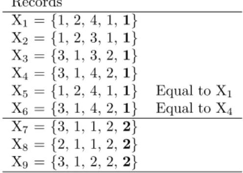
3.2. Association Rule Mining. To illustrate the algorithm, a simple data set shown in Table 1 is used as example.
Since the primary focus of the classifier PGN is on the rule’s confidence, we cannot use the downward closure property of the support metric to limit
the search space of confident association rules. The downward closure property specifies that by making an association rule more specific, i.e. adding additional antecedents, the support can not increase. The Apriori algorithm exploits this property by starting from very general rules and making them incrementally more specific until supports drops below a specified threshold. However, specifying such threshold will possible prevent us from learning all 100% confidence rules, which violates the goal of PGN.
Table 1. Example data set. The final attribute is the class attribute Records X1 ={1, 2, 4, 1,1} X2 ={1, 2, 3, 1,1} X3 ={3, 1, 3, 2,1} X4 ={3, 1, 4, 2,1} X5 ={1, 2, 4, 1,1} Equal to X1 X6 ={3, 1, 4, 2,1} Equal to X4 X7 ={3, 1, 1, 2,2} X8 ={2, 1, 1, 2,2} X9 ={3, 1, 2, 2,2}
PGN starts by adding all records to the set of association rules. For each class, a separate set of association rule is generated. In our example, the first four records are added as rules for class 1. Records X5 and X6 correspond to X1
and X4 respectively and are therefore not added since this would only result in
duplicate rules. The final three records are added to the rule set for class 2. This is illustrated in Figure 1.
Fig. 1. Adding records to the appropriate rule set
Next for each class, the intersection of every pair of rules is taken (cf. Definition 5). If the intersection results in a new rule which is not present in the rule set, it is added. This process continues until no more intersections are possible. The result of this step for the example data set is shown in Figure 2.
Definition 5: Intersection “∩”. R1∩R2 =R3 such that ∀x 3 j ∈R3 it holds that x3j = ( x1j if x1j =x2j − if x1j 6=x2j
Fig. 2. Creating new association rules through intersection
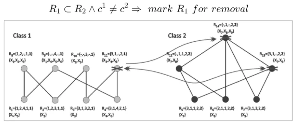
3.3. Pruning. In the pruning stage of PGN, association rules are re-moved from the rule set in two steps.
Firstly, all rules with a confidence less than 100% are removed, and sec-ondly rules for which a more general version is present in the rule set are also pruned. Pruning for confidence is performed in accordance with Definition 6. Application of this pruning step is illustrated in Figure 3. After all comparisons between rules from different classes are made, all rules marked for removal are pruned.
Definition 6: Pruning for confidence. R1⊂R2∧c
1
6
=c2 ⇒ mark R1 f or removal
Fig. 3. Pruning for confidence
It can easily be proven that pruning for confidence results in association rules with confidence equal to 100%.
P r o o f. Pruning for confidence removes rules with confidence less than 100%.
Assume that R1 ⊂ R2 and c 1
6
= c2. Since every rule is either a record from data setD or an intersection between two rules, we know that the support
of every rule is at least 1. From this follows that a record Xi exists such that
R2 ⊆Xi. Given that R1 ⊂R2, it follows thatR1⊂Xi. However, since R2 ⊆Xi
and c1 6=c2, we know thatR1⊆Xi cannot hold and conf idence(R1, D)<1.
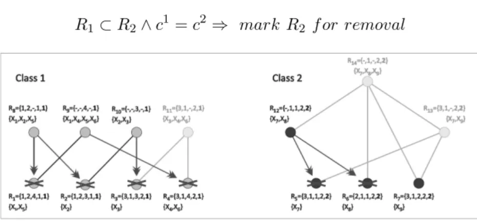
After all rules with a confidence level less than 100% are removed, a second pruning step is performed which retains only the most general rules. Pruning for general rules is performed as detailed in Definition 7. Application of this pruning step is illustrated in Figure 4. After all pairs of rules within each class are compared, all rules marked for removal are pruned.
Definition 7: Pruning for general rules. R1⊂R2∧c
1
=c2 ⇒ mark R2 f or removal
Fig. 4. Pruning for general rules
As a result of these two pruning steps, only general and highly confident rules are retained. For the example data set, the rules in Table 2 were retrieved after pruning.
Table 2. Association rules after pruning Rule Support Support set R1 ={1, 2, –, 1,1} 3 {X1, X2, X5} R2 ={–, –, 4, –,1} 4 {X1, X4, X5, X6} R3 ={–, –, 3, –,1} 2 {X2, X3}
X9 ={3, 1, 2, 2,2} 1 {X9} R5 ={–, 1, 1, 2,2} 2 {X7, X8}
3.4. Classification. To classify new instances with the pruned rule set, the definition for the size of an association rule must be introduced first. The association rule size corresponds to the number of non-class attributes which have a non-missing value.
Definition 8: Association Rule Size. |Rl|= n xlj|1≤j≤J−1, xlj 6=−o
This allows us to define an intersection percentage between a record Xi
and an association rule Rl:
Definition 9: Intersection Percentage.
IP(Xi, Rl) = 100∗
|Xi∩Rl|
Rl
To classify a new instance, the intersection percentage between the test case and every rule is calculated. This allows for three different scenarios:
– When the maximum intersection percentage occurs only once for one single rule, the class of this rule becomes the predicted class for the new instance. – When the maximum intersection percentage occurs multiple times, but only for rules from the same class, the class of these rules becomes the predicted class for the new instance.
– When the maximum intersection percentage occurs multiple times for rules from different classes, the supports of these rules are summed per class. The class with the highest aggregated support becomes the predicted class for the new instance.
Note that this classification scheme also uses association rules which do not cover the test case perfectly for classification purposes.
Let’s illustrate this classification method with the pruned rule sets in Ta-ble 2. Assume a new instanceXi={1,2,1,2,?}which needs to be classified (“?”
marks the unknown value of the class label). Firstly, the intersection percentage between Xi and every rule is calculated and shown in Table 3. The maximum
intersection percentage is 0.667 and occurs for rules R1 and R5 which belong to
different classes. Considering only the rules with an intersection percentage of 0.667, the summed support for class 1 is 3 and the summed support for class 2 is 2. Consequently, the new instance is predicted to belong to class 1.
Table 3. Classification ofXi ={1,2,1,2,?} Rl Xi∩Rl IP(Xi, Rl) Support R1 ={1, 2, –, 1, 1} {1, 2, –, –, ?} 0.667 3 R2 ={–, –, 4, –, 1} {–, –, –, –, ?} 0 4 R3 ={–, –, 3, –, 1} {–, –, –, –, ?} 0 2 R4 ={3, 1, 2, 2, 2} {–, –, –, 2, ?} 0.250 1 R5 ={–, 1, 1, 2, 2} {–, –, 1, 2, ?} 0.667 2
4. Empirical Analysis. The goal of this section is to empirically analyze the performance of PGN.
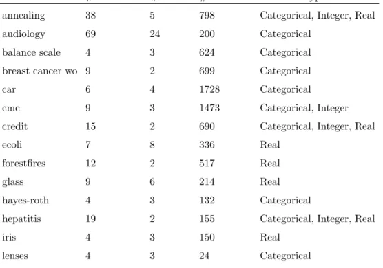
The experiments were performed on various data sets from the UCI Ma-chine Learning Repository [11]. The used data sets are described in Table 4. Data sets containing continuous attributes were discretized first by means of the Chi-merge method [14]. This discretization method is based on the χ2 statis-tic and uses a Chi-square threshold as stopping rule. In our experiments, the Chi-square threshold was set to 95%.
Table 4. Data sets
Data set # attributes # classes # instances Attribute type
annealing 38 5 798 Categorical, Integer, Real
audiology 69 24 200 Categorical
balance scale 4 3 624 Categorical
breast cancer wo 9 2 699 Categorical
car 6 4 1728 Categorical
cmc 9 3 1473 Categorical, Integer
credit 15 2 690 Categorical, Integer, Real
ecoli 7 8 336 Real
forestfires 12 2 517 Real
glass 9 6 214 Real
hayes-roth 4 3 132 Categorical
hepatitis 19 2 155 Categorical, Integer, Real
iris 4 3 150 Real
mammographic 5 2 961 Integer
monks1 6 2 432 Categorical
monks2 6 2 601 Categorical
monks3 6 2 554 Categorical
soybean 35 19 307 Categorical
tae 5 3 151 Categorical, Integer
tic tac toe 9 2 958 Categorical
votes 15 2 435 Categorical
wine 13 3 178 Integer, Real
winequality-red 11 6 1599 Real
zoo 16 7 101 Categorical, Integer
The goal of the experiments is to compare PGN against other classifiers and to find significant differences between the classifiers in terms of accuracy. For these purposes the methodology suggested by Demˇsar [8] is followed. First, unbiased estimates of the classifiers’ accuracies will be estimated by means of a five-fold cross validation for the observed datasets. Next, the Friedman test is used to detect statistically significant differences between the classifiers in terms of average accuracy. The Friedman test is a non-parametric equivalent of the repeated-measures ANOVA test, but is based on the ranking of the algorithms for each data set instead of the true accuracy estimates. In his paper, Demˇsar discusses several reasons why the ANOVA test is inappropriate for comparing multiple classifiers and why analyses should be performed on the ranking infor-mation instead of the overall accuracies. The interested reader is referred to [8]. If according to the Friedman test, differences between the classifiers exist, we use the Nemenyi test to compare each classifier with all other classifiers. The Nemenyi test controls for family-wise error in multiple hypothesis testing and is similar to the Tukey test for ANOVA. The results of the Nemenyi test are shown by means of critical difference diagrams.
The classifiers to compare with are representatives of different classifica-tion schemes, as follows:
– Associative classifiers: PGN and CMAR (using support threshold 1% and confidence threshold 50%);
– Decision Rules: One R, JRip (pruned and unpruned), Decision Table; NNge;
– Decision Trees: REP Tree, J48 (pruned and unpruned), LAD Tree; – Nearest Neighbor learners: IBk, KStar;
– Bayes: Na¨ıve Bayes, Bayes Net, HNB, WAODE, LBR; – Ensemble methods (Bagging): Random Forest;
– Support Vector Machines: SMO;
– Neural Networks: Multilayer Perceptron.
Experiments were made using the following programs:
– program realization of PGN in data mining environment PaGaNe [18]; – the program realization of CMAR in the LUCS-KDD Repository
(http://www.csc.liv.ac.uk/∼frans/KDD/);
– for all other classifiers their Weka implementation are used [26]. All classifiers received the discretized data set to begin with.
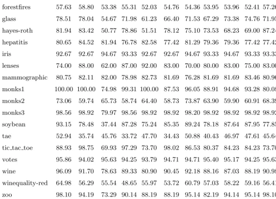
Table 5 shows the average accuracies of five-fold cross validation for ex-amined classifiers over chosen datasets.
Table 5a. Average accuracies of five-fold cross validation (first 11 classifiers) classifier PGN CMAR One R JRip- Dec. JRip- NNge REP J48- J48- LAD
dataset unpr. Table pruned Tree pruned unpr. Tree
annealing 96.24 95.99 83.71 99.00 98.37 98.12 97.24 97.62 98.12 98.75 98.12 audiology 75.50 59.18 47.00 68.50 61.00 69.50 67.00 62.50 72.00 72.00 71.50 balance scale 77.89 86.70 60.10 72.76 66.83 71.95 70.68 67.15 66.18 69.87 82.69 breast cancer wo 96.43 93.85 91.85 92.85 92.42 93.28 94.99 93.99 94.28 94.71 94.85 car 92.59 81.77 70.03 87.44 91.43 86.75 94.33 88.2 90.8 93.17 90.45 cmc 49.90 53.16 47.25 45.55 49.42 50.38 44.81 50.17 51.60 48.07 54.86 credit 87.54 87.10 85.51 81.45 85.8 85.07 80.14 85.07 85.36 83.91 86.67 ecoli 79.76 81.26 60.42 75.91 76.50 80.07 77.70 79.17 77.09 78.28 81.27
forestfires 57.63 58.80 53.38 55.31 52.03 54.76 54.36 53.95 53.96 52.41 57.26 glass 78.51 78.04 54.67 71.98 61.23 66.40 71.53 67.29 73.38 74.76 71.95 hayes-roth 81.94 83.42 50.77 78.86 51.51 78.12 75.10 73.53 68.23 69.00 87.24 hepatitis 80.65 84.52 81.94 76.78 82.58 77.42 81.29 79.36 79.36 77.42 77.42 iris 92.67 92.67 94.67 93.33 92.67 92.67 94.67 93.33 94.67 93.33 93.33 lenses 74.00 88.00 62.00 87.00 92.00 83.00 70.00 80.00 83.00 75.00 83.00 mammographic 80.75 82.11 82.00 78.98 82.73 81.69 76.28 81.69 81.69 83.46 80.96 monks1 100.00 100.00 74.98 99.31 100.00 87.53 96.05 88.91 94.68 93.28 80.08 monks2 73.06 59.74 65.73 58.74 64.40 58.73 73.87 63.90 59.90 60.91 68.39 monks3 98.56 98.92 79.97 98.56 98.92 98.92 98.20 98.92 98.92 98.92 98.92 soybean 93.15 78.48 37.44 87.28 75.24 85.35 89.24 78.18 87.64 87.95 77.85 tae 52.94 35.74 45.76 33.72 47.70 34.43 50.88 40.43 46.97 47.61 45.64 tic tac toe 88.93 98.75 69.93 97.29 73.70 98.02 86.53 80.37 84.23 84.23 73.70 votes 95.86 94.02 95.63 94.25 93.79 94.71 94.71 95.40 95.17 94.25 95.63 wine 96.09 91.70 78.63 89.33 80.90 90.45 92.18 88.16 87.03 88.19 90.98 winequality-red 64.98 56.29 55.54 48.65 55.97 53.72 60.79 57.03 58.22 59.16 56.41 zoo 98.10 94.19 73.29 90.14 88.19 88.19 95.14 82.19 94.14 95.14 98.10
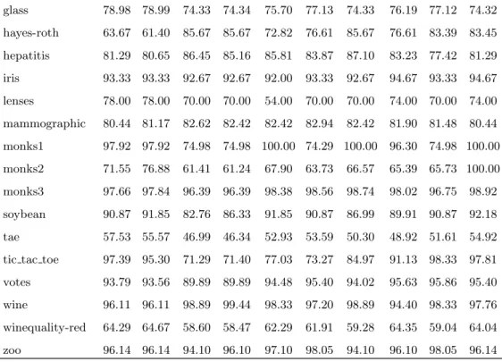
Table 5b. Average accuracies of five-fold cross validation (next 10 classifiers) classifier IBk KStar Na¨ıve Bayes HNB WAO LBR Rand. SMO Mult.
dataset Bayes Net DE Forest perc.
annealing 98.25 98.75 91.61 91.11 97.62 96.99 96.87 97.62 99.12 99.12 audiology 76.50 76.00 64.50 71.00 68.00 71.50 65.00 73.50 76.50 78.50 balance scale 85.26 86.70 90.54 90.54 87.02 88.14 90.54 75.48 89.42 98.72 breast cancer wo 95.85 95.28 97.14 97.14 95.13 95.85 97.14 95.42 95.99 96.28 car 92.94 86.81 85.19 85.30 92.24 90.11 91.95 93.52 92.59 99.83 cmc 47.12 50.31 50.45 50.31 52.96 52.68 52.55 48.68 53.50 47.73 credit 82.90 84.78 86.38 86.38 84.93 85.94 86.23 85.51 85.94 86.09 ecoli 79.76 80.36 84.84 84.54 79.77 82.75 84.84 80.36 84.24 80.67 forestfires 56.69 56.68 58.02 58.21 56.29 60.73 58.02 58.42 61.11 58.01
glass 78.98 78.99 74.33 74.34 75.70 77.13 74.33 76.19 77.12 74.32 hayes-roth 63.67 61.40 85.67 85.67 72.82 76.61 85.67 76.61 83.39 83.45 hepatitis 81.29 80.65 86.45 85.16 85.81 83.87 87.10 83.23 77.42 81.29 iris 93.33 93.33 92.67 92.67 92.00 93.33 92.67 94.67 93.33 94.67 lenses 78.00 78.00 70.00 70.00 54.00 70.00 70.00 74.00 70.00 74.00 mammographic 80.44 81.17 82.62 82.42 82.42 82.94 82.42 81.90 81.48 80.44 monks1 97.92 97.92 74.98 74.98 100.00 74.29 100.00 96.30 74.98 100.00 monks2 71.55 76.88 61.41 61.24 67.90 63.73 66.57 65.39 65.73 100.00 monks3 97.66 97.84 96.39 96.39 98.38 98.56 98.74 98.02 96.75 98.92 soybean 90.87 91.85 82.76 86.33 91.85 90.87 86.99 89.91 90.87 92.18 tae 57.53 55.57 46.99 46.34 52.93 53.59 50.30 48.92 51.61 54.92 tic tac toe 97.39 95.30 71.29 71.40 77.03 73.27 84.97 91.13 98.33 97.81 votes 93.79 93.56 89.89 89.89 94.48 95.40 94.02 95.63 95.86 95.40 wine 96.11 96.11 98.89 99.44 98.33 97.20 98.89 94.40 98.33 97.76 winequality-red 64.29 64.67 58.60 58.47 62.29 61.91 59.28 64.35 59.04 64.04 zoo 96.14 96.14 94.10 96.10 97.10 98.05 94.10 96.10 98.05 96.14
Table 6 shows the ranks of these classifiers over the data sets. Let’s men-tion that if two or more classifiers have equal accuracies, they share corresponded average ranks.
Table 7 shows the average rank for each classifier over the 25 UCI data sets. The Friedman test has aχ2 value of 95.579 with 20 degrees of freedom. For this degree of freedom the null hypothesis critical value is α0.10 = 28.412. This
indicates that there are statistically significant differences in accuracy among these 21 classifiers.
The rejecting of null-hypothesis of Friedman test gives the assurance to make post-hoc Nemenyi test. Figure 5 shows the results of the Nemenyi test.
CD0.10shows the groups of classifiers that are not significantly different atp=0.1.
From these results we see that PGN is competitive with techniques such as Neural Networks (Multilayer Perceptron), Support Vector Machines (SMO), Ensemble methods (Random Forest) and Bayes techniques and statistically outperforms more of the representatives of Decision Trees and Decision Rules.
T a b le 6 . T h e ra n k s o f cl a ss ifi er s ov er th e d a ta se ts cl a ss ifi er d a ta se t PG N CM AR On eR JR ip -u np ru ned Dec .T ab le JR ip -p ru ned NN ge RE PT ree J4 8-p ru ned J4 8-u np ru ned LA DT ree IB k KS ta r Na iv eB aye s Bay esN et HN B W A OD E LB R Ra nd For est SM O Mu lt. per cep tro n a n n ea li n g 1 7 1 8 2 1 3 6 9 1 4 1 2 9 4 .5 9 7 4 .5 1 9 2 0 1 2 1 5 1 6 1 2 1 .5 1 .5 a u d io lo g y 5 2 0 2 1 1 3 1 9 1 2 1 5 1 8 7 .5 7 .5 9 .5 2 .5 4 1 7 1 1 1 4 9 .5 1 6 6 2 .5 1 b a la n ce sc a le 1 2 8 .5 2 1 1 4 1 9 1 5 1 6 1 8 2 0 1 7 1 1 1 0 8 .5 3 3 7 6 3 1 3 5 1 b re a st ca n c. 4 1 7 2 1 1 9 2 0 1 8 1 2 1 6 1 5 1 4 1 3 7 .5 1 0 2 2 1 1 7 .5 2 9 6 5 ca r 6 .5 2 0 2 1 1 5 1 0 1 7 2 1 4 1 1 4 1 2 5 1 6 1 9 1 8 8 1 3 9 3 6 .5 1 cm c 1 3 3 1 8 2 0 1 4 9 2 1 1 2 7 1 6 1 1 9 1 0 .5 8 1 0 .5 4 5 6 1 5 2 1 7 cr ed it 1 2 1 1 .5 2 0 1 0 1 4 .5 2 1 1 4 .5 1 3 1 8 3 1 9 1 7 4 .5 4 .5 1 6 8 .5 6 1 1 .5 8 .5 7 ec o li 1 3 .5 7 2 1 2 0 1 9 1 1 1 7 1 5 1 8 1 6 6 1 3 .5 9 .5 1 .5 3 1 2 5 1 .5 9 .5 4 8 fo re st fi re s 9 3 1 9 1 4 2 1 1 5 1 6 1 8 1 7 2 0 1 0 1 1 1 2 6 .5 5 1 3 2 6 .5 4 1 8 g la ss 3 4 2 1 1 5 2 0 1 9 1 7 1 8 1 4 9 1 6 2 1 1 1 .5 1 0 8 5 1 1 .5 7 6 1 3 h ay es -r o th 8 6 2 1 9 2 0 1 0 1 3 1 4 1 7 1 6 1 1 8 1 9 3 3 1 5 1 1 .5 3 1 1 .5 7 5 h ep a ti ti s 1 3 .5 5 9 2 1 8 1 8 .5 1 1 1 5 .5 1 5 .5 1 8 .5 1 8 .5 1 1 1 3 .5 2 4 3 6 1 7 1 8 .5 1 1 ir is 1 7 1 7 3 9 .5 1 7 1 7 3 9 .5 3 9 .5 9 .5 9 .5 9 .5 1 7 1 7 2 1 9 .5 1 7 3 9 .5 3 le n se s 1 2 2 2 0 3 1 5 1 6 .5 7 5 1 0 5 8 .5 8 .5 1 6 .5 1 6 .5 2 1 1 6 .5 1 6 .5 1 2 1 6 .5 1 2 m a m m o g r. 1 7 8 9 2 0 3 1 2 2 1 1 2 1 2 1 1 6 1 8 .5 1 5 4 6 6 2 6 1 0 1 4 1 8 .5 m o n k s1 3 .5 3 .5 1 8 .5 7 3 .5 1 5 1 1 1 4 1 2 1 3 1 6 8 .5 8 .5 1 8 .5 1 8 .5 3 .5 2 1 3 .5 1 0 1 8 .5 3 .5 m o n k s2 4 1 9 9 .5 2 0 1 2 2 1 3 1 3 1 8 1 7 6 5 2 1 5 1 6 7 1 4 8 1 1 9 .5 1 m o n k s3 1 1 4 .5 2 1 1 1 4 .5 4 .5 1 4 4 .5 4 .5 4 .5 4 .5 1 7 1 6 1 9 .5 1 9 .5 1 3 1 1 9 1 5 1 8 4 .5 so y b ea n 1 1 7 2 1 1 2 2 0 1 5 9 1 8 1 1 1 0 1 9 6 3 .5 1 6 1 4 3 .5 6 1 3 8 6 2 ta e 5 1 9 1 6 2 1 1 1 2 0 8 1 8 1 4 1 2 1 7 1 2 1 3 1 5 6 4 9 1 0 7 3 ti c ta c to e 9 1 2 1 6 1 6 .5 3 1 0 1 4 1 2 .5 1 2 .5 1 6 .5 5 7 2 0 1 9 1 5 1 8 1 1 8 2 4 v o te s 1 .5 1 5 .5 4 1 3 .5 1 7 .5 1 0 .5 1 0 .5 7 9 1 3 .5 4 1 7 .5 1 9 2 0 .5 2 0 .5 1 2 7 1 5 .5 4 1 .5 7 w in e 1 0 1 3 2 1 1 6 2 0 1 5 1 2 1 8 1 9 1 7 1 4 8 .5 8 .5 2 .5 1 4 .5 7 2 .5 1 1 4 .5 6 w in eq .-re d 1 1 7 1 9 2 1 1 8 2 0 8 1 5 1 4 1 0 1 6 4 2 1 2 1 3 6 7 9 3 1 1 5 zo o 1 .5 1 3 2 1 1 7 1 8 .5 1 8 .5 1 1 .5 2 0 1 4 1 1 .5 1 .5 7 7 1 5 .5 9 .5 5 3 .5 1 5 .5 9 .5 3 .5 7
Table 7. Average ranks on 25 UCI data sets for PGN and 20 other classifiers PGN CMAR One R JRip- Dec. JRip- NNge REP J48- J48- LAD
unpr. Table pruned Tree pruned unpr. Tree Avg.Rank 7.96 10.52 17.18 14.40 13.94 13.78 12.50 14.20 12.48 12.08 10.20
IB k K Star Na¨ıve Bayes HNB WAO LBR Rand. SMO Mult.
Bayes Net DE Forest perc.
Avg.Rank 9.66 9.36 11.48 11.18 9.86 8.82 8.68 8.92 7.60 6.20
Fig. 5. Comparison PGN and 20 other classifiers (Nemenyi test)
Finally, note that in contrast with the some other classifiers (especially associative classifiers), PGN is a parameter free classifier.
5. Conclusions. The goal of this article is to question the support-first principle used by many associative classifiers when mining for association rules. Instead, a new associative classifier, called PGN, was developed which turns the common approach around and focuses primarily on the confidence of the association rules and only in a later stage on the support of the rules. The main purpose of this research was to provide a proof of concept for this new
approach and collect evidence about its potential.
The experimental results are very positive and show that PGN is com-petitive with some of the more advanced classification methods such as Neural Networks, Support Vector Machines, Ensemble methods and Bayes techniques, while statistically outperforming more of the representatives of Decision Trees and Decision Rules. At the same time, PGN has the advantage over the other Associative Classifiers that it is parameter free.
In general, the results provide evidence that the confidence-first approach yields interesting opportunities.
Now that the proof of concept is given, future research must focus on the computational efficiency of the algorithm, since this was not the focus during this research. Particularly, the association rule mining step is computationally expensive in the current implementations. Another interesting direction for future research concerns an adjustment of the current algorithm which to mine for highly confident association rules which are not necessarily 100% confidence results.
R E F E R E N C E S
[1] Agrawal R., T. Imielinski, A. Swami.Mining association rules between sets of items in large databases. In: Proceedings of the 1993 ACM SIGMOD international conference on Management of data, ACM, New York, USA, 1993, 207–216.
[2] Agrawal R, R. Srikant. Fast algorithms for mining association rules in large databases. In: Proceedings of the 20th International Conference on Very Large Data Bases (VLDB ’94), Morgan Kaufmann Publishers Inc, San Francisco, CA, USA, 1994, 487–499.
[3] Aha D., D. Kibler, M. Albert. Instance-based learning algorithms. Ma-chine Learning,6 (1991), No 1, 37–66.
[4] Antonie M.-L., O. Za¨ıane. Text document categorization by term asso-ciation. In: Proceedings of the 2002 IEEE International Conference on Data Mining (ICDM’02), IEEE Computer Society, Washington, DC, USA, 2002, 19–26.
[5] Antonie M.-L., O. Za¨ıane, R. Holte.Learning to use a learned model: A two-stage approach to classification. In: Proceedings of the Sixth
Inter-national Conference on Data Mining, IEEE Computer Society, Washington, DC, USA, 2006, 33–42.
[6] Boser B., I. Guyon, V. Vapnik.A training algorithm for optimal margin classifiers. In: Proceedings of the fifth annual workshop on Computational learning theory (COLT ’92), ACM, New York, NY, USA, 1992, 144–152. [7] Coenen F., P. Leng.Obtaining best parameter values for accurate
classi-fication. In: Proceedings of the Fifth IEEE International Conference on Data Mining (ICDM’05), IEEE Computer Society, Washington, DC, USA, 2005, 597–600.
[8] Demˇsar J.Statistical comparisons of classifiers over multiple data sets. J. Mach. Learn. Res.,7 (2006), 1–30.
[9] Depaire B., G. Wets, K. Vanhoof. Traffic accident segmentation by means of latent class clustering.Accident Analysis & Prevention,40(2008), No 4, 1257–1266.
[10] Fayyad U., G. Piatetsky-Shapiro, P. Smyth.Advances in knowledge discovery and data mining. Chapter. From Data Mining to Knowledge Dis-covery: An Overview, American Association for Artificial Intelligence, Menlo Park, CA, USA, 1996, 1–34.
[11] Frank A., A. Asuncion. UCI machine learning repository, 2010.
[12] Goethals B. Efficient Frequent Pattern Mining. PhD thesis, Transna-tionale Universiteit Limburg, 2002.
[13] Han J., J. Pei, Y. Yin. Mining frequent patterns without candidate gen-eration. SIGMOD Rec., 29(2000), No 2, 1–12.
[14] Kerber R.ChiMerge: discretization of numeric attributes. In: Proceedings of the tenth national conference on Artificial intelligence (AAAI’92), AAAI Press, 1992, 123–128.
[15] Li W., J. Han, J. Pei. CMAR: Accurate and efficient classification based on multiple class-association rules. In: Proceedings of the 2001 IEEE Inter-national Conference on Data Mining, IEEE Computer Society, Washington, DC, USA, 2001, 369–376.
[16] Liu B., W. Hsu, Y. Ma. Integrating classification and association rule mining. In: Proceedings of the ACM Int. Conf. on Knowledge Discovery and Data Mining (SIGKDD ’98), New York City, NY, 1998 80–86. (The CBA system can be downloaded fromhttp://www.comp.nus.edu.sg/dm2). [17] Maimon O., L. Rokach. Decomposition methodology for knowledge
dis-covery and data mining. Data Mining and Knowledge Disdis-covery Handbook, Springer US, 2005, 981–1003.
[18] Mitov I. Class Association Rule Mining Using Multi-Dimensional Num-bered Information Spaces. PhD thesis, Hasselt, Belgium, 2011.
[19] Morishita S., J. Sese. Transversing itemset lattices with statistical met-ric pruning. In: Proceedings of the nineteenth ACM SIGMOD-SIGACT-SIGART symposium on Principles of database systems, ACM, New York, NY, USA, 2000, 226–236.
[20] Quinlan J.Induction of decision trees.Mach. Learn.,1 (1986), 81–106. [21] Quinlan J.C4.5: programs for machine learning. Morgan Kaufmann
Pub-lishers Inc., San Francisco, CA, USA, 1993.
[22] Rak R., W. Stach, O. Zaane, M.-L. Antonie.Considering re-occurring features in associative classifiers. In: Advances in Knowledge Discovery and Data Mining, Lecture Notes in Computer Science, Vol.3518, 2005, Springer, Berlin/Heidelberg, 2005, 240–248.
[23] Tang Z., Q. Liao. A new class based associative classification algorithm.
IAENG International Journal of Applied Mathematics, 36 (2007), No 2, 15–19.
[24] Thabtah, F., P. Cowling, Y. Peng. MCAR: multi-class classifi-cation based on association rule. In: Proceedings of the ACS/IEEE 2005 International Conference on Computer Systems and Applications (AICCSA ’05), IEEE Computer Society, Washington, DC, USA, 2005. doi: 10.1109/AICCSA.2005.1387030
[25] Wang J, G. Karypis.Harmony: Efficiently mining the best rules for clas-sification. In: Proc. of SDM, 2005, 205–216.
[26] Witten I., E. Frank. Data Mining: Practical machine learning tools and techniques. Morgan Kaufmann, San Francisco, 2nd edition, 2005.
[27] Yin X., J. Han.CPAR: Classification based on predictive association rules. In: Proceedings of the SIAM International Conference on Data Mining, SIAM Press, San Francisco, CA, 2003, 369–376.
[28] Za¨ıane O., M.-L. Antonie. On pruning and tuning rules for associa-tive classifiers. In: Knowledge-Based Intelligent Information and Engineer-ing Systems, Vol. 3683, Lecture Notes in Computer Science, Springer, Berlin/Heidelberg, 2005, 966–973.
[29] Zimmermann A., L. De Raedt.CorClass: Correlated association rule min-ing for classification. In Discovery Science, Vol.3245, Lecture Notes in Com-puter Science, Springer, Berlin/Heidelberg, 2004, 60–72.
Iliya Mitov, Krassimira Ivanova
Institute of Mathematics and Informatics Bulgarian Academy of Sciences
Acad. G. Bonchev Str., Bl. 8 1113 Sofia, Bulgaria
e-mails: [email protected] [email protected]
Koen Vanhoof, Benoit Depaire IMOB, Hasselt University Hasselt, Belgium
e-mails: [email protected] [email protected]
Received July 5, 2013