Identification of undesirable behaviour in CCTV footage using Deep Learning

(1)

Middlesex University Research Repository

An open access repository of

Middlesex University research

http://eprints.mdx.ac.uk

Mateusz, Bulat (2018) Identification of undesirable behaviour in CCTV footage using Deep Learning. Masters thesis, Middlesex University.

Final accepted version (with author’s formatting)

This version is available at:http://eprints.mdx.ac.uk/26401/

Copyright:

Middlesex University Research Repository makes the University’s research available electronically. Copyright and moral rights to this work are retained by the author and/or other copyright owners unless otherwise stated. The work is supplied on the understanding that any use for commercial gain is strictly forbidden. A copy may be downloaded for personal, non-commercial, research or study without prior permission and without charge.

Works, including theses and research projects, may not be reproduced in any format or medium, or extensive quotations taken from them, or their content changed in any way, without first obtaining permission in writing from the copyright holder(s). They may not be sold or exploited commercially in any format or medium without the prior written permission of the copyright holder(s).

Full bibliographic details must be given when referring to, or quoting from full items including the author’s name, the title of the work, publication details where relevant (place, publisher, date), pag-ination, and for theses or dissertations the awarding institution, the degree type awarded, and the date of the award.

If you believe that any material held in the repository infringes copyright law, please contact the Repository Team at Middlesex University via the following email address:

[email protected]

The item will be removed from the repository while any claim is being investigated.

(2)

Mateusz Bulat 1 | P a g e

Identification of Undesirable Behaviour

in CCTV Footage Using Deep Learning

By Mateusz Bulat

M00347487

A thesis submitted to Middlesex University

in partial fulfilment of the requirements for the degree of Master of Science (by Research) Faculty of Science and Technology

December 2018 Supervised by: Dr Aboubaker Lasebae

(3)

Abstract

Anomaly detection in CCTV recording is a difficult and challenging subject due to the issue of the vast amount of the data that must be processed, and the expertise required to analyse it. CCTV operators undergo a long and extensive training to spot anomalous behaviour in CCTV recording, but even with the acquired expertise, on average an operator will lose up to 45% of screen activities after 12 minutes, and up to 95% after 22 minutes.

This research investigates a novel pipeline technique to process CCTV recording using a combination of different unsupervised machine learning techniques. The principle pipeline technique evaluated consists of and Autoencoder as a feature extractor, in combination with a one-class Support Vector Machine (SVM), and Hidden Markov Model (HMM). Extracted Autoencoder features are categorised using the SVM to determine anomaly per frame, followed by temporal smoothing of the SVM frame categorisation with the HMM. The system achieves an accuracy of 61.38% and an AUC of 0.59. The system was evaluated by comparing the results produced by the system with regards to labels provided with a dataset. The results collected from the comparison were used to produce an area under curve value.

The report will look in to comparing the results of using a pre-trained CNN (VGG16) and Autoencoder for purpose of feature extraction.

Being unsupervised, the system requires very little human interference and it was designed to teach itself how to differentiate an anomaly from a non-anomalous event. The only human input that the system requires was the selection of parameters for all the algorithms. The rest was left for

algorithm to decide based on a set criterion. The obtained results, which while inevitably inferior to the performance of comparable supervised systems (i.e. where the anomaly class is explicitly labelled in the training data), provides an effective proof of concept of pipelining that can be used for purpose of unsupervised anomaly detection of a CCTV image frame.

(4)

Acknowledgements

I would like to thank all my supervisors for all the support that they have provided me with.

Especially Dr David Windridge who provided me with invaluable knowledge of machine learning, Dr Aboubaker Lasebae who provided me with support regarding academic research.

I would also like to thank my mother whose support allowed me to complete my work.

Thanks also goes to Faculty of Science and technology at Middlesex University which financed my Master’s degree, and provided me with the equipment and support.

(5)

Table of Figures

Figure 1 Example of feedforward neural network (Michael Nielsen, 2017)... 15

Figure 2 Sigmoid activation function (Andrej Karpathy, 2015) ... 16

Figure 3 Tanh activation function (Andrej Karpathy, 2015) ... 17

Figure 4 ReLU activation function (Andrej Karpathy, 2015) ... 17

Figure 5 Visualization of the AlexNet network (Alex Krizhevsky, Ilya Sutskever and Geoffrey E Hinton, 2017) ... 21

Figure 6 Autoencoder diagram (Deeplearning4j Development Team., 2017) ... 23

Figure 7 Example of SVM using Linear kernel Polynomial Kernel (Eric Kim, 2015) ... 26

Figure 8 Example of SVM using Polynomial kernel (Xing Liu, 2014) ... 27

Figure 9 Example of using one class SVM (scikit-learn, 2010) ... 28

Figure 10 Examples of anomalous and non-anomalous sets of Ped1 set... 34

Figure 11 Diagram demonstrating the first experiment ... 37

Figure 12 Example feature vector of values extracted from Autoencoder in SVMLight format ... 39

Figure 13 Diagram demonstrating the second experiment ... 39

Figure 14 Diagram demonstrating the third experiment ... 41

Figure 15 Diagram demonstrating the fourth experiment. ... 44

Figure 16 Example loss function vs time graph for sixth training example ... 45

Figure 17 100th frame of sixth training example ... 46

Figure 18 Loss function of 31st training example ... 47

Figure 19 Frame 30 of 31st _{train example ... 47}

Figure 20 Frame 80 of 31st _{train example ... 47}

Figure 21 Loss function graph for sixth training example using 4th _{model ... 48}

Figure 22 Loss function graph for 31st training example using 4th _{model ... 48}

Figure 23 Loss function for 1st test example ... 48

Figure 24 Loss function for 14th test example ... 48

Figure 25 Frame 111 of Test001 example ... 49

Figure 26 Frame 137 of Test014 example ... 49

Figure 27 ROC curve for SVM trained on Autoencoder's features. ... 50

Figure 28 Example of anomalous frame ... 50

Figure 29 Example of anomalous frame ... 51

Figure 30 ROC Curve for layer 19 test ... 53

Figure 31 ROC Curve for layer 20 test ... 56

Figure 32 ROC for a combination of Autoencoder, SVM, and HMM where SVM parameters act as a threshold. ... 58

Figure 33 ROC for a combination of Autoencoder, SVM, and HMM where HMM parameters act as a threshold. ... 59

Figure 34 Graph presenting the values produced by Autoencoder, SVM, and HMM for Test 3 example ... 59

(8)

Figure 37 Graph presenting the values produced by Autoencoder, SVM, and HMM for Test 29 example ... 61 Figure 38 Graph presenting the values produced by Autoencoder, SVM, and HMM for Test 35 example ... 61

(9)

Tables

Table 1 Transition probability matrix for Sunny and Rainy example ... 30

Table 2 Emission probability matrix ... 31

Table 3 Autoencoder model design details ... 35

Table 4 Parameters selected for SVM trained of features provided by the Autoencoder ... 38

Table 5 Parameters selected for SVM ... 41

Table 6 Start Probabilities ... 42

Table 7 Transition Probabilities ... 43

Table 8 Emission Probabilities ... 43

Table 9 SVM parameters ... 43

Table 10 Results of each PED1 example produced by SVM trained using features provided by the Autoencoder. ... 52

Table 11 VGG16 layer 19 best overall accuracy results ... 54

Table 12 VGG16 layer 20 best overall accuracy results ... 57

Table 13 Results of example test example produced by combination of Autoencoder, SVM, and HMM ... 63

(10)

List of abbreviations

CCTV Close circuit television SVM Support vector machine HMM Hidden Markov Model ReLU Rectified linear units MSE Mean Squared Error

ROC Receiver Operating Characteristic Curve VGG16 Visual Geometry Group 16

RNN Recurrent Neural Network TP True positives

FN False negatives TN True negatives FN False negatives

Tanh hyperbolic tangent function MSE Mean Squared Error

CNN Convolutional neural networks LSTM Long short term memory

(11)

1. Introduction

1.1 Background and Motivation

According to report(BSIA CCTV statistics report July 2013. 2013) there are approximately 4 - 5.9 million CCTV cameras in Britain. A number of these cameras are actively monitored by CCTV

operators but large number of these would not be actively monitored due to lack of importance. The task of simultaneously monitoring multiple feeds from CCTV cameras is a very mentally demanding, tedious and monotonous task. Which is why according to study published in Security Oz magazine (Ainsworth, 2002) “after 12 minutes of continuous video monitoring an operator will often miss up to 45% of screen activity, after 22 minutes of viewing, up to 95% is overlooked” which proves the already established fact that people are very bad at prolonged cognitive tasks.

The purpose of this project was to test the effectiveness of machine learning to detect anomalous activity from a CCTV. Machine learning is a branch of artificial intelligence which concentrates on simulating the way that people learn. Neural networks simulate the explicit learning processes of the brain.

Recent advancements in gaming technology and graphics cards made training neural networks accessible to average researcher. It reduced training time from months to few weeks, and

sometimes couple hours. Neural networks are applied to a number of advanced tasks, for example, recurrent networks such as one developed by (Donahue et al., 2016) are now capable of describing a video clip in nearly real-time. A convolutional network described by (Spanhol et al., 2016) can detect cancerous cells in medical images.Both of these are examples of machine learning being used for tasks which recently were dominated by human experts.

Training a neural network for the purpose of anomaly detection is a challenging task because anomalies are rare events, and it is difficult to provide an example for every single type of anomaly. Therefore, a better approach is to train a network on non-anomalous examples which are easier to obtain and then allow a network to detect anomalies by comparing it to the expected pattern. This project will propose to use compressed features of Autoencoder with a combination of Support vector machine for the purpose of training an unsupervised model to detect anomalies in video recording.

(12)

The result of this combination will then be compared with a combination of the Convolutional neural network with a one class SVM, in order to evaluate the newly developed system against a supervised system.

1.2 The research Aim, Objectives & Research questions

This project aims to propose an anomaly detection technique combined of an unsupervised

Autoencoder as feature extraction, and one class Support vector machine as a classification system. The motivation to use Autoencoder comes from the algorithm’s strength of learning input features without any prior labelling. The Support vector machine is used for binary classification. However, it also has a one class variant that is ideally suited for anomaly categorization purposes, its usefulness coming from ability to categorize data only non-anomalous data labels available.

The questions that this project is aiming to answer are following:

1. How effective is unsupervised fully connected Autoencoder for feature extraction for anomaly detection?

2. Based on features provided by an Autoencoder can an SVM be used for classification purposes, and how well will the system have performed?

3. How do the results of the combination of Autoencoder and one class SVM compare to pre-trained Convolutional network and one class SVM?

1.3 Scientific Contribution

The report provides reader with a novel idea of how combination of different machine learning techniques can be used for purpose of anomaly detection. The combination combines the fully connected Autoencoder, SVM, and HMM.

The developed system was then compared against combination of a pre-trained CNN and SVM, for purpose of comparing the effectiveness of the two approaches.

For purpose of the first question the Autoencoder developed was unable to provide the necessary values to identify the anomaly in the frame, but the Autoencoder did learn the correct features. This allowed for the Autoencoder to be used for purpose of the second experiment.

For the second question the Autoencoder developed for purpose of first question was used again. For this question, the Autoencoder was used as a feature extractor, which worked very well with combination of SVM. Where Autoencoder was used for purpose of extracting the useful features off the frame, and then the one class SVM was used for purpose of classification.

The first experiment was the comparison of the combination of Autoeoncder and one class SVM against a pre-trained CNN and one class SVM. The aim of this experiment was to compare if the

(13)

trained Autoencoder and pre-trained CNN network makes difference for purpose of feature extraction for one class SVM.

The aim of the last experiment was to explore the idea of using HMM to provide smoothing of the results that one class SVM would provide, from the combination of techniques used in second experiment.

1.4 Thesis Outline

The report will go as follow. The chapter two will introduce different machine learning techniques, as well as evaluation methods used for purpose of comparing the results between different developed techniques.

The chapter three will explain the methodology used to confirm the research questions, and experiments that were used to achieve the answers to the research questions.

The fourth chapter is the discussion of the outcomes from the experiments performed in third chapter.

The last chapter is a conclusion and further research that could be performed to further develop the technique.

(14)

2. Literature Review

2.1. Anomaly Detection

Anomaly detection is a process of detecting anomalous reading, behaviour, or actions from an input data. The anomaly can be anything that does not conform to an expected pattern or other items of the dataset(Chandola, Banerjee and Kumar, 2009) . A well know example of anomaly detection is for bank and credit card fraud.

Deep neural networks are state of the art for general image classification due to their ability to process and learn complex features and relationships between data. It is more difficult to train a neural network to detect anomalies. This is due to an imbalance of dataset as anomalous cases are, by definition, significantly fewer and more diffuse compared to non-anomalous cases.

Due to this imbalance, an anomaly detection networks are usually only trained on non-anomalous examples. Only then the model is applied to anomalous cases. This type of training is called one-class training it was proven in number of cases such as one in “Video anomaly detection based on ULGP-OF Descriptor and One-class ELM”(Siqi Wang, En Zhu and Jianping Yin, 2016) . However, standard deep learning approaches are not appropriate for this form of training, due to the discriminative nature of the architectures such as CNN or deep networks. (Khan and Madden, 2014)

Another challenging aspect of training a system for the purpose of anomaly detection in CCTV recording is because the CCTV is a continuous stream of data. Therefore, an anomaly might be related to an action that happened some frames in the past, and the system might have to consider temporal context.(Jiajun Sun, Jing Wang and Ting-chun Yeh, )

(15)

2.2. Neural Networks

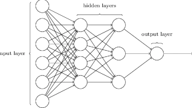
The neural network is an important subset of artificial intelligence, the purpose of this field being to model networks after human brain and nervous system (Christos Stergiou and Dimitrios Siganos, 2017) Figure 1 presents an example of a neural network made of multiple layers, where each layer contains several nodes. Neural network learns by using algorithms such as feedforward or

backpropagation.

2.2.1. Training Types

There are different paradigms in machine learning for processing data; the three main approaches are:(Katrina Wakefield, 2017)

• Supervised

• Semi-Supervised

• Unsupervised

Supervised learning depends on data being labelled and associating the result of the algorithm with a label. The system will adjust the parameters of the model such as weights to associate inputs with this specific label. The advantage of such system is that the system can be improved by applying more data with labels. The disadvantage of this approach is a human input requirement of labelling the data which might introduce a human error. (Katrina Wakefield, 2017)

Semi-supervised learning learns using partially labelled dataset, but then it will use its own

knowledge of the features to label the dataset and learn even more features. The advantage of this approach is that it requires a very small dataset compared to the supervised dataset. The

disadvantage is that the model might misclassify some inputs due to lack of labels in the dataset. (Katrina Wakefield, 2017)

Unsupervised learning does not use labels to learn the features of the dataset but looks at similarities of the input values. It will then categorise the same type of features into one type of class. For example, if there are two types of cars in the dataset green and red, the system might categorise the input into two different classes, due to distinct colours being presented. The

advantage of this system is that it does not require any human input, therefore, reduces the chance of a human error being introduced. The disadvantage of the system is the lack of control that supervised, and semi-supervised learning provides, and the system learns the feature on its own which might introduce some misclassification. (Katrina Wakefield, 2017)

(16)

2.2.2. Layers

Neural networks have three types of layers, input layers which takes an input value, hidden layers which processes the data and learns the features, and an output layer which outputs the

classification of an input Figure 1. (Standford University, 2015)

(17)

2.2.3. Activation Functions

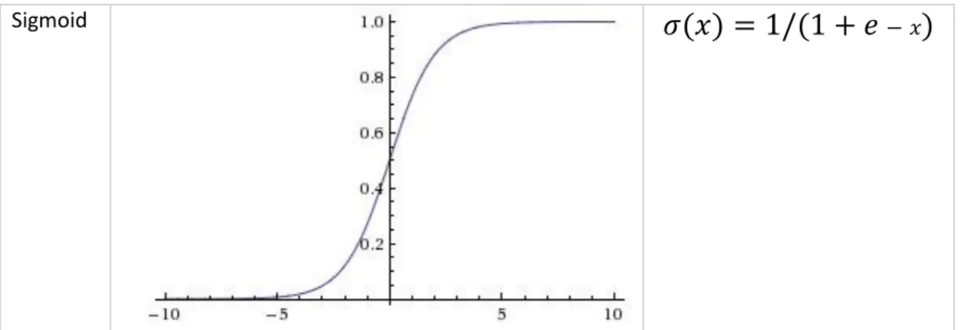
A hidden layer processes the data provided by input layers by passing it through an activation function using a process called forward propagation or feedforward. (Michael Nielsen, 2017) There a multiple different activation functions with different properties. Some examples of activation functions are Sigmoid Figure 2, RELU Figure 3, and Tanh Figure 4. The list here was used in designing of the Autoencoder model.

The sigmoid function Figure 2 is useful to combine the result in between two values of 0 and 1 which bounds the information in between two values. It provides control of how the data is being

processed. The same control of the data might cause the issues of vanishing gradient when the value is close to the horizon of the curve. This issue might prevent the network from learning any useful features when using algorithms such as backpropagation which relies on gradient big enough to affect the weights of the model. (Andrej Karpathy, 2015)

The sigmoid function is useful in bounding the result of the network in between two values, which is a useful activity for the last layer of the network which is used for classification purposes.

Sigmoid

_{𝜎(𝑥) = 1/(1 + 𝑒}

_{− 𝑥}

₎

(18)

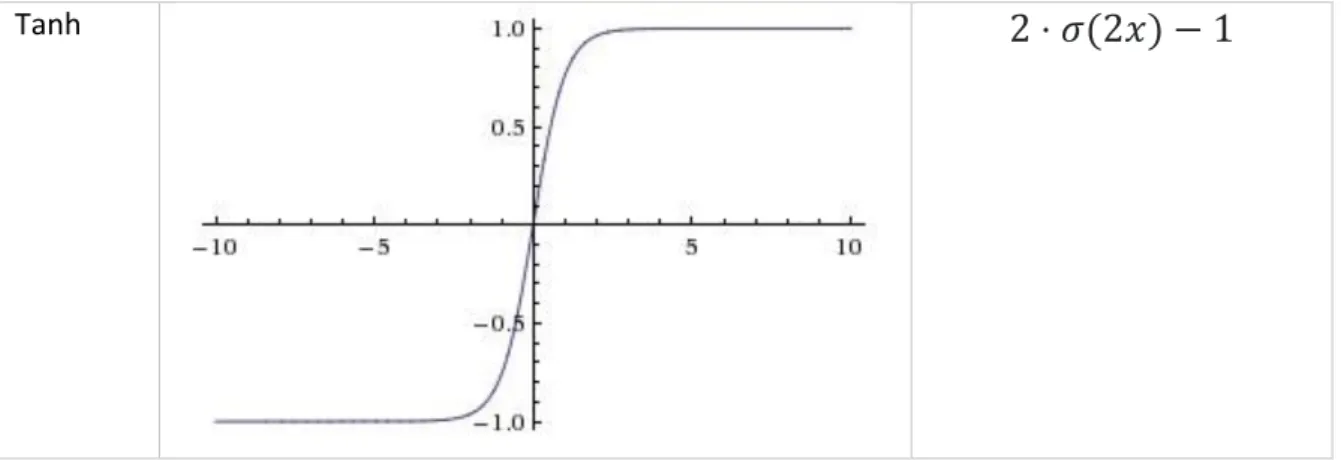
Tanh activation function Figure 3 is very similar to Sigmoid. Both functions are bound in between two values in case of Tanh it is -1 and +1. The Tanh is not zero-cantered therefore it does not make the weights of the layers “zig-zag” from negative to positive which is a case of the sigmoid function. (Andrej Karpathy, 2015)

Tanh

_{2 ⋅ 𝜎(2𝑥) − 1}

Figure 3 Tanh activation function (Andrej Karpathy, 2015)

The Rectified Linear Units (ReLU) Figure 4 is simple yet powerful activation function. The activation function takes the input value and checks if the value is lower than 0, then the output value is 0, otherwise the input is linear with slope of 1. The ReLU was found to increase the coverage of stochastic gradient decent compared to sigmoid or Tanh functions, due to its linear approach and non-saturating form. (Alex Krizhevsky, Ilya Sutskever and Geoffrey E Hinton, 2017)

ReLU

_{𝑓(𝑥) = 𝑚𝑎𝑥(0, 𝑥)}

(19)

2.2.4. Feedforward, Backpropagation, and Gradient Descent

Feedforward is an algorithm that is used for the purpose of inputting the data into a model and outputting a result. The feedforward model only works one way, and it does not receive any additional data during the process. Once the result is provided with the feedforward algorithm with adjusting its parameters to improve the performance of the model.

The feedforward backpropagation is an algorithm that will input the data into the model, and then calculate the error of the model and backpropagate the error to adjust the weights of the model to improve the accuracy of the system.

The weights of each layer will be adjusted using gradient descent. Which will take the derivative of the model, calculate the partial derivative of the layer, and adjust the weights of the layer to improve the performance of the model.(Standford University, 2015) (Jahnavi Mahanta, 2017)

2.2.5. Weights and Biases

Bias is a trainable constant value which allows shifting decision boundary to fit the network better. (Nate Kohl, 2010)

Weights are used to specify the importance of certain features over others; neural network uses weights to adjust the outcome of the network classification. Weights are being adjusted by backpropagation algorithm to improve the classification of the model.(Rojas and Feldman, 1996) There are several different variants of gradient descent. Batch gradient descent computes gradient by using the entire dataset, which is very computationally and expensive memory task due to the size of the dataset. Stochastic gradient descent, on the other hand, performs gradient update of a fraction of the dataset which is faster and less memory and computational task. (Sebastian Ruder, 2017)

(20)

2.2.6. Loss Function

The loss function is used for the purpose of measuring the degree of how well the network fits the dataset. (Yixuan Hu, 2017) In the case on an unsupervised model such as Autoencoder, the Loss function will calculate how well the model has reconstructed the input value, and produce the score to represent the accuracy of the output value.

Few examples of loss functions are:

Mean Squared Error (MSE) is an example of loss function

𝑀𝑆𝐸 ≔1

𝑛∑ 𝑒𝑡

2 𝑛

𝑡=1

Cross-Entropy Loss is another example of loss function 𝐻_𝑦′(𝑦) ≔ − ∑ 𝑦_𝑖′

𝑖

log(𝑦𝑖)

2.2.7 Evaluation methods

For machine learning algorithm to be meaningful it requires a method to evaluate its effectiveness. For that reason, there are number of methods that can be used to evaluate effectiveness of the system.

ROC (receiver operating characteristic) curve

Is a method used to evaluate the performance of the machine learning algorithm. The method uses a selected threshold value to provide four variables:

1. True positives (TP) 2. False negatives (FN) 3. True negatives (TN) 4. False negatives (FN)

The threshold value is used to generate multiple outcomes of above-mentioned variables.

The ROC is used for purpose of plotting a curve graph which is used to generate an AUC (Area under curve) value.

For this graph two values are required sensitivity and specificity. The value of sensitivity is calculated using following function:

(21)

The value of specificity is calculated using following function: TN/(TN+FP)

To produce the graph the value of sensitivity is plotted against specificity for each threshold value used.

For purpose of this research a single value was selected, for SVM it was the value of nu, and for HMM it was the values of emission probabilities and transition probabilities.

In case of SVM the values were selected by running a for loop 100 times and changing the sensitivity of the SVM by adjusting the nu value from 0.01 to 0.02, until the value of 1.0. For each test a new SVM model had to be trained, and each model took about 2 minutes of training.

Same methodology was used for purpose of HMM, but there were 4 values in total and each test, was run for ever value selected.

(Jennifer Hallinan, 2014) AUC (Area under curve)

Is a value that is produced out of the ROC diagram used for purpose of evaluating the effectiveness of an prediction system. The AUC is calculated combining an area of trapezoid where the base of the trapezoid is the base of the graph and two points of the ROC curve are the two highest points of the trapezoid.

All the areas of the trapezoid are then combined into a single value that measure the systems discriminative ability.

If the value of AUC is smaller or save as 0.5, it will mean that the system is guessing the outcome of the classification. A value larger than 0.5 is what’s being desired from the system.

(Suzanne Ekelund, 2012a)

2.3. Convolutional Neural Network

The origin of the convolutional neural network goes all the way back to Hubel and Wiesel’s (Hubel and Wiesel, 1959) experiments on cats. In which they tried to understand the way that brain process the visual input. They discovered that the brain processes visual inputs using layers which have different purposes such as edges detection. This neuroscientific experiment leads the way to several computer vision experiments such “Machine Perception of Three-Dimensional Solids” also

sometimes called Block World PhD paper by Lawrence Gilman Roberts. All these experiments lead to the development of convolutional networks such as LeNet5 in 1998.(Lecun et al., 1998)

(22)

Convolutional neural networks (CNN) is primarily used for the purpose of image classification; it is usually trained using supervised learning. The network uses a combination of convolutional and max-pooling layers to extract unique features of the image and produce a kernel that can be used for image classification. The network learns the features of the image by backpropagating the error back through the network and adjusting weights on each node to increase the accuracy of the model. (Alex Krizhevsky, 2015)

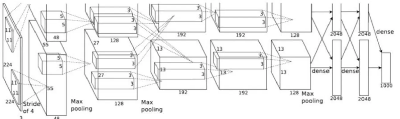
The convolutional networks became popular in 2012 when AlexNet network won the ImageNet competition by outclassing all the other competitors. Since 2012 most of the models submitted to this ImageNet competition were CNN’s. AlexNet was built by Alex Krizhevsky, who was a researcher at the University of Toronto.(Alex Krizhevsky, Ilya Sutskever and Geoffrey E Hinton, 2017)

The AlexNet was based on an early network called LeNet designed by Yann LeCun in 1990, the network was much shallower than AlexNet only five layers and was applied to the problem of number recognition.

Figure 5 Visualization of the AlexNet network (Alex Krizhevsky, Ilya Sutskever and Geoffrey E Hinton, 2017)

Convolutional networks have been used for the purpose of anomaly detection in several papers such as “Deep-anomaly: a Fully Convolutional neural network for fact anomaly detection in Crowded scenes” by (Mohsen Fayyaz, Mahmood Fathy and Reinhard Klette, 2016) . The CNN used in this paper was pre-trained, and it was used for extracting the features out of the dataset to use them in the fully connected network. The reason for not using a pure CNN network was due to totally supervised learning requirement of CNN which cannot be applied to unsupervised learning which anomaly detection dataset require.

The convolutional neural network’s strength is the high accuracy of image classification and feature extraction, but due to the need for supervised learning, it cannot be applied to unsupervised task on anomaly detection.

(23)

A CNN network involves several steps to perform its actions, such as ReLU activation, pooling (Down Sampling), Flattening, and fully connection. (Alex Krizhevsky, 2015)

ReLU activation function was already discussed previously.

Pooling is used for purpose of reducing spatial size of the representation, which improves the computation of the network by reducing the number of parameters. The pooling layers are usually placed in between convolutional layers. A popular pooling function is a max function which take the maximum value of the stride, for example if the stride is 2, then the pooling layer will take a

maximum value of 2 by 2 matrix. Other available function is average pooling.(Alex Krizhevsky, 2015) Flattening the CNN network operates on matrix data, but for the CNN network to classify something it requires a classification module to perform this operation such as a dense or fully connected layer. The fully connected layer can only perform its operation on flatten or vector data, for that reason a data must be reshaped from 2 dimensional into a single dimensional format which is called

flattening. (Alex Krizhevsky, 2015)

Fully connected layer is type of layer where each node is connected to another layer, and for purpose of CNN the fully connected layer is used for classification purposes.

2.4. Autoencoder

The Autoencoder is a network that tries to reconstruct input by reducing the reconstruction error. Autoencoder is an unsupervised network meaning it does not use any labels to associate them with features learnt. It will minimise the reconstruction error and use it as a measure the correctness of the outcome. (Skymind, 2016)

This type of network is made of encoding and decoding stages. An encoding stage will reduce the number of input features and decoding stage will try to decode the compressed features to match the input values.(Skymind, 2016)

Autoencoders are usually made of several fully connected layers, which take an input, process it and pass it along to next layer. There are some examples of convolutional autoencoders (Turchenko and Luczak, 2015) that instead of using fully connected layers use convolutional layers for the purpose of autoencoding.

These type of convolutional autoencoders use the convolutional layers, and pool layers, as well as unconvolutional and unpooling layers for the purpose of encoding and decoding.

(24)

Convolutional layers are used in convolutional networks and have been successfully used for the purpose of image classification. Therefore, applying this layer to autoencoder would be beneficial as proven by (Turchenko and Luczak, 2015) . The issue with this approach is that to use a convolutional layer in autoencoding requires the use of an unconvolutional layer and unpooling layers. These layers are not well understood and not included in many libraries, therefore, require a great amount of troubleshooting to make them work. (Turchenko and Luczak, 2015)

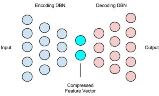
Figure 6 Autoencoder diagram (Deeplearning4j Development Team., 2017)

An autoencoder in Figure 6 is an example of stacked autoencoder. In this type of autoencoder, layers are “stacked” on top of each other. The first three layers will gradually compress the features which is called encoding. The decoding stage will take the compressed vector features and try to

reconstruct the input value by calculating the loss function.

Autoencoder network is a popular choice for anomaly detection, due to its ability to learn the input features without of any labels. Anomalies are rare therefore training a network to detect them is a challenging task as the unbalance in datasets does not provide enough features to learn the anomalies.

Therefore, for anomaly detection, autoencoders are trained to learn the features of non-anomalous results. The model trained in such a way will then be applied to anomalous examples, and the reconstruction error will be used for the purpose of measuring the probability of anomaly in the data. This is caused by model not being able to correctly reconstruct the data due to never seeing an

(25)

anomaly before, which is a good indication that something is going wrong in the data being processed.

Autoencoders are difficult to train due to their unsupervised nature. Because they do not need labels to learn the features, they will learn by compressing and decompressing the features and adjusting their weights depending on loss function error value. To achieve a good result, the network will have to pick up correct features and learn how to reconstruct them. If incorrect features are learnt by the network will not produce correct results.

Autoencoders are useful for the purpose of compressing the features and extracting them for different purposes. Therefore, they can be used to provide a unique representation of the data for another model to categorise it correctly. The reconstruction error can also be used for the purpose of categorising the possibility of an error occurring in the frame.

(Zhengying Chen et al., 2015) explain how an Autoencoder can be used for the purpose of anomaly detection. An autoencoder in this paper is trained on non-anomalous dense trajectories, and then in the testing phase, the model is applied to anomalous examples which the reconstruction error is different from the base provided by non-anomalous examples.

The issue of using autoencoder for anomaly detection is lack of control of what features the model will learn because the model is trained using unsupervised learning.

(26)

2.5. Support Vector Machine

Support vector machine is a binary algorithm used for the purpose of classification and separation of data. The SVM uses a hyperplane which is a line that splits the input variable space, and provides a classification of data. The distance between two points of different clusters is called a margin. The best margin is the one that has the largest value between two groups of classes. SVMs may be further enhanced by implemented a Kernel. The algorithm learns by transforming the problem using linear algebra.

The one class SVM provides an effective and inexpensive solution to a problem classification, where only way category is provided. Because the one-class SVM can be trained on a single category. It means that it can be used for purpose of anomaly detection training, where training set is combined of non-anomalous examples, and the test set is a mix of both anomalous and non-anomalous examples. As the one-class SVM is trained on non-anomalous examples, it knows very well on how to detect these types of examples, but once the model is introduced to anomalous examples, it will place this example outside of the border of non-anomalous examples, therefor marking this example something out of ordinary. (Schoelkopf et al., Nov 29, 1999) (Tax, 2001)

2.5.1. Linear Kernel

Linear Kernel is the simplest example of a kernel in SVM. The kernel defines the distance measure between new data and the support vector. The Linear kernel will split the data with a linear hyperplane.

(27)

Mateusz Bulat 26 | P a g e Figure 7 Example of SVM using Linear kernel Polynomial Kernel (Eric Kim, 2015)

In Linear kernel, the separation of data is done using a hyperplane; in the case of a Polynomial kernel, the kernel can separate the data more aggressively by being able to use a curved, non-linear separator. For this kernel to fit the data correctly, the degree parameter must be picked. Degree function is defined as “d” in the function below.

(28)

Mateusz Bulat 27 | P a g e Figure 8 Example of SVM using Polynomial kernel (Xing Liu, 2014)

The SVM was used in a number of different papers for the purpose of anomaly detection. In a paper by (Yingying Miao and Jianxin Song, 2014) SVM was used for the purpose of classifying output provided by Adaptive genetic simulated annealing algorithm (ASAGA). Using SVM for the purpose of anomaly detection provided very good results, as well as it made easy to retrain the results for different purposes. This paper used the same UCSD anomaly detection dataset used for the purpose of evaluation in this report.

(29)

Mateusz Bulat 28 | P a g e Figure 9 Example of using one class SVM (scikit-learn, 2010)

One important aspect of SVM is that it can be adapted for the purpose of one class classification. That is when the dataset only contains a single class, and the SVM learns how to detect that specific class. If an example is tested on a system that does not fit the class that SVM was trained on the SVM will mark it as an anomaly. (Microsoft, 2017)

2.6. Recurrent Neural Network

The purpose of the recurrent neural network is to process continuous data such as sound, movies, and graphs. The unique aspect of this network is that it remembers the error from past processed examples, and it uses these experiences to classify the result. RNN uses an LSTM layer (Long-Short term memory) for the purpose of carrying the state from past examples and combines it with a current example. (J•urgen Schmidhuber and Sepp Hochreiter, 1997)

Until the introduction of LSTM in 1997, the recurrent neural network was suffering from a problem of vanishing gradient. The vanishing gradient is when a gradient calculated at the top layers of the network is so small that bottom layers are unable to learn any useful features, which affects the performance of the entire network.

(30)

A video dataset is made of multiple frames, and anomaly might be a continuous action such as someone cycling or skateboarding. If only one frame is used for anomaly detection, this frame might not have enough information to provide certainty that the anomaly is present or not. Use of RNN might thus improve a chance of correctly classifying an action as anomaly or not. This approach was considered by (Chong and Tay, 2017) where a combination of RNN and CNN was used to detect anomalies by considering not only a single frame but the whole video recording as one continuous action.

For RNN to show its full potential, it requires a dataset that is very well labelled. In case of anomaly detection problem that is very unlikely to be provided. Full anomaly detection thus depends on one class classification which in case of RNN cannot be achieved as RNN requires labels for training purposes.

Technically RNN can be used for the purpose of one-class anomaly detection but only when there is a support system that can perform anomaly detection on a single frame, and then use that decision to train a recurrent neural network, on features extracted by the system, and label provided by the support system.

(31)

2.7. Hidden Markov Model

A Hidden Markov model (HMM) is a finite model that describes a probability distribution over an infinite number of possible sequences. HMM was used in a number of functions such as biological sequence analysis(Byung-Jun Yoon, 2009) .

An HMM is made of four variables:

• Observable

• State transition probability

• Initial state distribution

• Emission probability

In Markov model (MM) the system is only based on states, where HMM is based on observables. Observables are variables that indirectly select the probability of a state. For example, if MM were built to predict the weather the MM would use states such as rainy or sunny, but if these variables are unavailable we can use HMM which instead of depending on states would depend on

observables, which are related variables for example clothes that people wear in rain might different than clothes wore during sunny weather, and these observables could be used to predict the

weather pattern.

State transition probability are values that represent a probability of changing from one state to another. The total value of transition probability per state should not exceed a value of 1. For example, if the model measures a transition from one weather pattern to another such as sunny to rainy the transition between rainy and rainy might be 0.4 and rainy and sunny might be 0.6, which totals at the value of 1. The transition between sunny and sunny might be 0.6, and sunny to rainy might be 0.4, which again must total in 1.

The transition probability is usually represented in the form of a matrix. Table 1 Rainy Sunny

Rainy 0.4 0.6 Sunny 0.6 0.4

(32)

The initial state distribution is values that represent the initial probability of each state; these values must total together to the value of 1. To bring the weather example, if the place that the data is coming from is usually sunny then the initial state for sunny could be 0.7 and the initial state of rainy is could be 0.3.

Hidden Markov model which works by using variables called observables, instead of relying on states to provide the prediction.

Using the weather example, if the weather data is unavailable, but the data of what people wear is available, then the clothing can be used for the purpose of predicting the weather. Clothing, in this case, is an observable variable.

Observable variables require emission probability matrix that is used for the purpose of stating what’s the probability of seeing an observable value depending on the state. For example, for our observable, we have two values, someone wearing a t-shirt, and someone wearing a jacket.

Jacket T-shirt Rainy 0.7 0.3 Sunny 0.2 0.8

Table 2 Emission probability matrix

The total value for each state needs to equal to 1. Table 2 for example, total value for state Rainy is the combined value of observable Jacket (0.7) and observable T-Shirt (0.3) which totals together as the value of 1.

There is number of a different algorithms that can be used for the purpose of HMM such as Viterbi, The Forward Algorithm, The Forward-Backward Algorithm. (Hidden Markov Models. 2017)

(Ayse Elvan Gunduz Tugba Taskaya Temizel Alptekin Temizel, 2014) used HMM for the purpose of anomaly detection in the paper “Pedestrian Zone Anomaly Detection by Non-Parametric Temporal Modelling” for the purpose of combining the results extracted using feature extractors.

(33)

3. Anomaly Detection Experiments

This chapter will introduce the experiments that were used for purpose of this research project. The chapter will introduce the dataset used for all the experiments, followed by every experiment that was based on the dataset.

It takes time and resources to achieve a dataset which can be used for the purpose of anomaly detection; there arer number of parameters to consider such as human bias, the type of data in the dataset, the size of it, the time required for the purpose of creating the dataset. For that reason, it is easier and more reasonable to use already existing and established dataset which has been tested and used for a number of other researches. For that purpose, here are two datasets considered for the purpose of anomaly detection.

The Deeplearning4j library is developed by company called Skymind, a San Francisco-based business intelligence and enterprise software firm. The library is open-source, distributed deep-learning project in Java and Scala. The library supports several different deep learning techniques such as CNN, Autoencoders, RNN, and many others (Skymind, 2018) . The library and community behind the library provide several pre-build deep learning models inside of their model zoo, but it also allows for freedom of developing a model from scratch using a Java code. The library provides a support to Nvidia’s Cuda library which improves the speed at which the models are being trained. As of

November 2017, the Skymind joined the Eclipse foundation, which allowed it to establish its self as a number one deep learning library in Java ecosystem.(Chris Nicholson, 2017)

A LIBSVM library was selected for purpose of training the One class SVM. LIBSVM is an integrated software for support vector classification, (C-SVC, nu-SVC), regression (epsilon-SVR, nu-SVR) and distribution estimation (one-class SVM). It supports multi-class classification. The library is written in a Java language and is used in number of software such as scikit-learn (scikit-learn developers, 2018) or Rapidminer (RapidMiner, 2018) .

A library developed byadrianulbona on GitHub was selected for purpose of developing an implementation of an HMM. There aren’t a lot of well-developed libraries that allows for implementation of HMM, therefore this following library was selected due to its stability and simplicity of development.

(34)

A Java programming language was selected to its maturity and verticality, as well as authors knowledge of the language.

3.1. UCSD Anomaly Detection Dataset

The UCSD anomaly detection dataset was recorded from a stationary camera mounted at an elevation, overlooking pedestrian walkways. The crowd density varies from between clips, from few people to large crowd. The training set contains only pedestrians.

The weather conditions are good; no rain or fog which would hide aspects of the images. The dataset is in black and white. The recording took place during the day which provided good lighting conditions.

The dataset has a tree in the top right corner of video which hides some part of the path, but any events behind tree top are not being considered as part of anomalies.

Abnormal events are due to either:

• the circulation of non-pedestrian entities in the walkways

• anomalous pedestrian motion patterns

Anomalies include bikers, skaters, small carts, and people walking across a walkway or in the grass that surrounds it. A few clips also contain a wheelchair. All the anomalies are naturally occurring and not staged. The data was split into two subsets, each corresponding to a different scene. The video footage recorded from each scene was split into various clips of 200 frames each.

The two sets available are:

Peds1: clips of groups of people walking towards and away from the camera, and some amount of perspective distortion. Contains 34 training video samples and 36 testing video samples.

Peds2: scenes with pedestrian movement parallel to the camera plane. Contains 16 training video samples and 12 testing video samples.

(35)

Mateusz Bulat 34 | P a g e Figure 10 Examples of anomalous and non-anomalous sets of Ped1 set

For each clip, the ground truth annotation includes a binary flag per frame, indicating whether an anomaly is present in that frame. Also, a subset of 10 clips for Peds1 and 12 clips for Peds2 are provided with manually generated pixel-level binary masks, which identify the regions containing anomalies. This is intended to enable the evaluation of performance concerning the ability of algorithms to localise anomalies.(UCSD Anomaly Detection Dataset. 2010)

The accuracy of the model based on this dataset is measured using two factors.

Pixel level accuracy which is when a model detects the abnormally which covers 40% of the abnormality map.

Frame level accuracy which is when at least one pixel of the frame is considered as anomalous.

3.2. Subway-Exit

Subway-exit dataset is made of two actual surveillance video of subway station recorded by a camera at the entrance and exit gates.

The exit gate video is 43 minutes long. The base activities in the recordings are people exiting from the platform and coming up through the exit gates. Anomalous events mainly involve walking in from wrong direction and loitering.

(36)

The entrance video is 96 minutes long; it shows people going down and entering the platform. There are 66 rare events, mainly people walking in the wrong direction, people suddenly stopping, or running to the train. (A. Adam, 2010)

3.3. Dataset Conclusion

The UCSD anomaly detection dataset has been used in some research. It provides good quality recording as well as accurate ground truth labels. Compared to Subway-exit dataset which has more data available, but the ground truth labels are less accurate, or sometimes missing. The UCSD has an effective way of evaluating the performance of the model that was created, which allows comparing the different models against each other. For this research, UCSD dataset will be used as the main dataset, to be precise the PED 1 section of the dataset.

3.4. Autoencoder Experiment

The following methodology was used for testing performance of the Autoencoder as a source of features extractor.

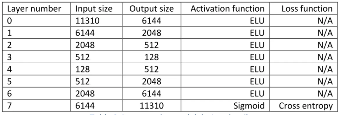
A fully connected Autoencoder was built using Deeplearning4j library. The network was made of 8 layers.

Layer number Input size Output size Activation function Loss function

0 11310 6144 ELU N/A 1 6144 2048 ELU N/A 2 2048 512 ELU N/A 3 512 128 ELU N/A 4 128 512 ELU N/A 5 512 2048 ELU N/A 6 2048 6144 ELU N/A

7 6144 11310 Sigmoid Cross entropy

Table 3 Autoencoder model design details

The following parameters were selected for network design. The weights were initialised using Xavier algorithm. The gradient was normalized by clipping L2 per layer. The optimization algorithm was Stochastic Gradient Descent. The updater was AdaDelta. Regulazation was selected, and the L2 algorithm was selected.

The learning rate was set to 0.001; the l2 parameter was set to 0.01, bias Learning Rate was set to 0.001, gradient normalization was set to 0.1, batch size was set to 256, a number of the epoch was set to 100.

(37)

The Autoencoder was trained using UCSD Ped 1 dataset which consists of a training and testing sets. The model was trained using training dataset. The testing test was then applied to produce the graphs.

The training set was split into two portions 70% training and 30% testing using the splitting feature provided as part of the library. The size of each frame of the dataset was size by approximately 50% to prevent memory allocation issues produced by the size of the Autoencoder parameters; the graphics card was equipped with 12Gb of video RAM, this was a limiting factor to a number of features that could have been used for training. Each image was normalized between values of 0 and 1, and then reshaped from the matrix into a vector.

The performance of the Autoencoder was evaluated by producing a temporal graph of combined loss function of each frame of the example. The graphs for training sets are available in Appendix A, and graphs for testing sets are available in Appendix B.

The graphs were then compared with the ground truth, to ensure that Autoencoder can produce a meaningful result.

(38)

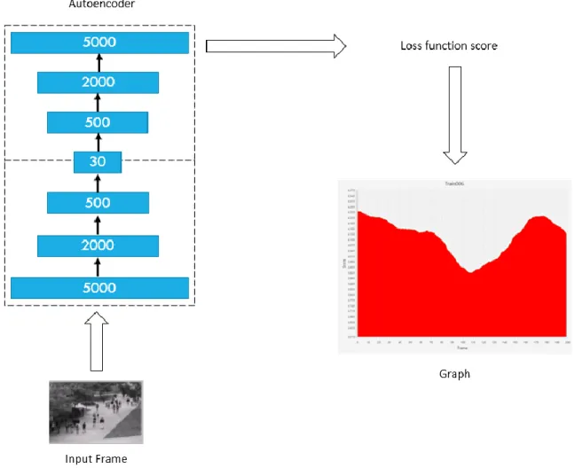
Mateusz Bulat 37 | P a g e Figure 11 Diagram demonstrating the first experiment

Figure 11 shows step by step how the experiment was performed.

The first step was to train the Autoencoder using UCSD dataset. Once the dataset was trained, every frame of the test portion of PED 1 dataset was run through the trained model. The Loss function score produced by the model was then collected, and once every frame of the example was tested and the values combined to produce the temporal graph.

(39)

3.5. Autoencoder and SVM Experiment

The following methodology was used for the purpose of testing the performance of a combination of Autoencoder as feature extractor and SVM for the purpose of anomaly detection.

The compressed representation of features produced by the Autoencoder was used for the purpose of training the SVM. The logic of this experiment is to find out the performance of the SVM on features provided by the Autoencoder.

The following parameters (Table 4) were selected for the training of one class SVM model. Parameter Value

SVM Type One class Cache size 80

Shrinking True Kernel type Polynomial

Nu 0.65

Eps 0.001

Gamma 2

Degree 3

Coef 1

Table 4 Parameters selected for SVM trained of features provided by the Autoencoder

The SVM was trained on a laptop equipped with Intel i5-3340M 2.7Ghz, and 16GB of RAM. The training time took approximately 2 minutes due to the high input compression achieved by the Autoencoder.

The one class SVM was trained using following features extracted from each frame. The format used for extracted features is called SVMLight which is a format recommended by an LIBSVM library, a library that was used to produce the SVM model. This format requires that every value of the vector needs to have a number assigned, also if the vector has a label or ground truth associated with it is has to be placed before the vector and separated by the space or empty character.

(40)

Mateusz Bulat 39 | P a g e 1:0.38 2:0.37 3:0.27 4:0.82 5:2.65 6:0.39 7:0.69 8:3.95 9:0.34 10:0.38 11:0.74 12:0.47 13:0.38 14:0.36 15:15.59 16:0.37 17:0.33 18:4.87 19:0.19 20:0.23 21:6.16 22:0.20 23:0.17 24:2.98 25:3.40 26:0.41 27:0.51 28:6.46 29:5.34 30:0.37 31:5.33 32:5.02 33:2.73 34:5.37 35:0.34 36:0.41 37:2.99 38:0.12 39:0.37 40:0.34 41:0.40 42:0.41 43:0.46 44:4.68 45:0.41 46:0.70 47:5.99 48:0.39 49:3.87 50:4.56 51:0.32 52:6.78 53:3.50 54:0.27 55:4.06 56:0.13 57:6.30 58:0.33 59:7.59 60:0.42 61:0.39 62:1.59 63:0.38 64:0.48 65:8.50 66:6.92 67:0.41 68:3.27 69:5.68 70:1.66 71:2.02 72:0.28 73:0.41 74:1.30 75:0.43 76:0.39 77:5.66 78:2.56 79:6.13 80:0.30 81:0.49 82:0.08 83:0.54 84:0.36 85:0.39 86:11.58 87:1.78 88:0.33 89:1.40 90:4.46 91:0.37 92:0.45 93:2.01 94:1.78 95:3.04 96:0.37 97:0.45 98:10.57 99:0.40 100:0.13 101:6.73 102:3.56 103:4.47 104:0.94 105:0.04 106:5.07 107:4.45 108:4.42 109:0.36 110:0.32 111:0.42 112:12.80 113:0.43 114:0.34 115:0.88 116:3.05 117:1.84 118:0.47 119:5.80 120:3.62 121:0.22 122:11.96 123:1.96 124:0.43 125:0.47 126:2.02 127:0.49 128:3.47

Figure 12 Example feature vector of values extracted from Autoencoder in SVMLight format

The accuracy and performance of the SVM were evaluated using the ground truth labels provided with the dataset. The results are going to be presented using receiver operating characteristic curve (ROC), from which an area under curve (AUC) value is going to be calculated. AUC is a value selected for the purpose of comparing different approaches based on this dataset.

(41)

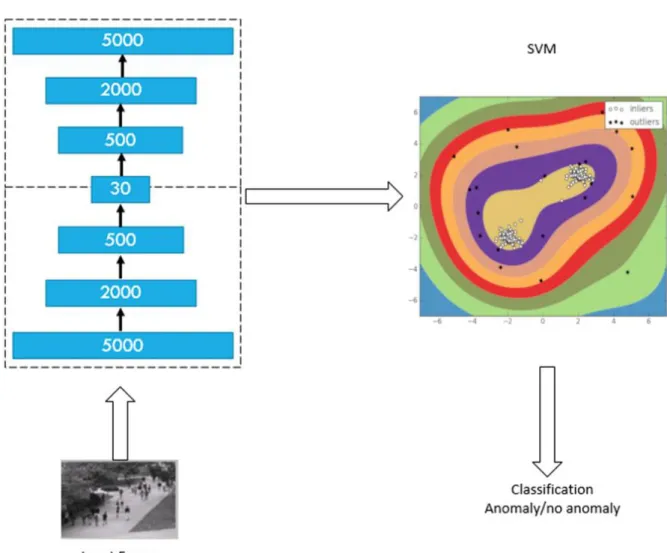
Figure 13 is a diagram demonstrating the second experiment. In this experiment, every frame was processed separately, but instead of using the loss function, the compressed values of the middle-hidden layer were used to train SVM. The SVM was trained using training set, and the test set was used to test the performance of the SVM, the system was evaluated by comparing the values produced by the SVM with the ground truth provided by the dataset.

3.6. CNN and SVM Experiment

Following methodology was used for the purpose of testing performance of a combination of CNN and SVM for the purpose of anomaly detection.

The purpose of this experiment was to compare the effectiveness of the Autoencoder as a feature extractor against other methods used for feature extraction. In case of this experiment, a CNN network will be used as a feature extractor. Usually, CNN’s are used for classification purposes, but they can also be used as feature extractors, by extracting values out of layers that aren’t used for classification purposes.

Once the values are extracted, they were used for the purpose of training an SVM network to classify if the frame is anomalous or not.

A model picked for this test was VGG16 which secured first the second place of ImageNet challenge in 2014(Karen Simonyan and Andrew Zisserman, 2014) . This model was pre-trained using ImageNet dataset. It was provided as part of zoo model in Deeplearning4j Library(Skymind, 2017)

The two layers selected for extraction purposes are layers 14 and 15 which are represented in the library as layers 19 and 20. Both layers are fully connected layers which provide features in vector format.

The extracted parameters were then used for the purpose of training an SVM, to predict if the frame contains anomaly or not.

The same library as in the second experiment was used to train and test the SVM. SVMLight data format was used to process the data provided by the CNN.

(42)

Parameter Value SVM Type One class Cache size 80

Nu 0.99

Eps 0.001

Gamma 7

Degree 2

Coef 1

Table 5 Parameters selected for SVM

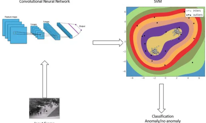
Figure 14 Diagram demonstrating the third experiment

Figure 14 demonstrated the design of the third experiment. Each frame was reduced in size to meet the input requirements of the CNN network. Each frame was processed separately. Once the frames were processed by the CNN, they were extracted and used for training and testing purposes of the SVM.

The experiment was evaluated by comparing the classification provided by SVM against the ground truth provided by the dataset. The result of comparison was then used to produce the ROC, which

(43)

then will be used to calculated AUC a value which is used for the purpose of evaluating the performance of the model against other models.

3.7. Autoencoder, SVM and HMM Experiment

Following methodology is used for the purpose of testing the effect of considering the relationship between the frame classification provided by the SVM. The combination of Autoencoder and SVM was only considered a single frame of the dataset without of considering the relation between frames. By not considering the relation between frames the accuracy of the system might be reduced, due to a fact that the Autoencoder only considers a single frame, and this single frame doesn’t contain any details about the past of the action that is currently happening in that certain frame.

To address this disadvantage, a new process was added to the system which considers the relationship between predictions provided by the combination of Autoencoder and SVM.

The selected process is a Hidden Markov model, a system used for the purpose of representing the probability of distribution over a sequence of observations.

A library provided by adrianulbona from Github was used for the purpose of building and testing the HMM. (Adrian Bona, 2015)

The outputs provided by the SVM was used as observables for the HMM.

The SVM provided double variables of 1.0 and -1.0, but due to requirements of the library the variables were converted from 1.0 to “positive”, and -1.0 to “negative”.

The two states selected for the purpose of HMM are called “Anomaly” and “No anomaly”. Following HMM parameters were selected.

The start probabilities are 0.1 for Anomaly and 0.9 for No Anomaly Table 6. Anomaly No Anomaly

0.1 0.9

Table 6 Start Probabilities

Table 7 contains the transition probabilities, used for the purpose of calculating a probability of changing from one state to another.

(44)

Anomaly No Anomaly

Anomaly 0.7 0.3

No Anomaly 0.2 0.8

Table 7 Transition Probabilities

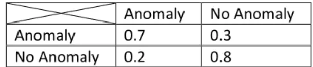
Table 8 contains emission probabilities selected for the purpose of calculating the relation between observables and states.

Positive Negative

Anomaly 0.4 0.6

No Anomaly 0.6 0.4

Table 8 Emission Probabilities

The probabilities values selected for purpose of this experiment were selected by running this experiment through all the available values between 0.1 and 0.9 using a simple loop statement. For every available combination of the probabilities, a test was performed by running the solution generated on the test set of the dataset and comparing the results against labels provided with the dataset. The final values selected in this experiment are the values which had the highest final score available generated from the system.

The dataset itself had couple of cases where the training set contained an anomalous case, for example in one set there was a cyclist visible for number of frames, which should not be happening in the dataset, due to idea that the autoencoder trained on this set might consider this as non-anomalous example.

The parameters for SVM were adjusted to provide improved results as presented in Table 9. As in previous experiments, the model was trained using training and testing vectors produced by Autoencoder, the values were formatted using SVMLight format.

Parameter Value SVM Type One class Cache size 80

Nu 0.67 Eps 0.001 Gamma 1 Degree 1 Coef 1 Table 9 SVM parameters

(45)

Mateusz Bulat 44 | P a g e Figure 15 Diagram demonstrating the fourth experiment.

Figure 15 shows the diagram demonstrating the fourth experiment. The first three sections of the experiment are same as in the third experiment. The frame is converted into a vector; the

autoencoder is trained and used to extract compressed feature representation, then SVM is trained using the vector values produced. The next step is to buffer all the frames for each example and input them into HMM which will provide series of values based on inputs provided by the SVM. This experiment was evaluated by comparing the values provided by the HMM against ground truth provided by the dataset. The comparison result will then be represented using ROC curve which will be used to calculate the AUC values.

(46)

4. Results and Discussion

4.1. Autoencoder Experiment

The Autoencoder produces meaningful results, the majority of the graphs generated by the Autoencoder for the training set having a flat graph without of any crest or troughs. A few graphs, however, did produce a crest or trough for example Figure 16.

Flat graphs in relation to the normal class training set are a good sign, as it means that the

Autoencoder did not have any difficulties with decoding the frames. As otherwise, the autoencoder would produce trough or crests which would mean that it tried to decode something that it never has seen before and it had difficulty in performing the decoding phase of the Autoencoder.

(47)

Figure 17 is the 100th_{frame from the 6}th_{training example. This frame received the lowest score out}

of the entire 6th_{example. While there is no anomaly in this frame, the Autoencoder had difficulty in}

reconstructing this frame. There is no straightforward way to pinpoint the exact reason why this score was produced, however it might be due to some people looking very different to features that Autoencoder saw before or it might be due to the amount of people in the frame.

Figure 17 100th frame of sixth training example

Figure 18 contains the result of training example 31. This training example contains a small trough between frame 50 and 80. Again because the Autoencoder is looking at the frame level anomaly it is hard to pin-point the exact reason why the score was selected, but if we look at Figure 19 and Figure 20 which show frame 30 and 80 of the example, we can clearly deduce that it might be caused by the number of people present in the frame.

(48)

Mateusz Bulat 47 | P a g e Figure 18 Loss function of 31st training example

Figure 19 Frame 30 of 31st _{train example} _{Figure 20 Frame 80 of 31}st _{train example} The same trough and crest were present in models trained before final model. Figure 16 and Figure 18 are produced using sixth and final model, Figure 21 and Figure 22 are produced using a fourth model, and the trough and crests are visible.

(49)

Mateusz Bulat 48 | P a g e Figure 21 Loss function graph for sixth training

example using 4th _model

Figure 22 Loss function graph for 31st training example using 4th _model

When the Autoencoder was presented with a test set of the dataset, the model had a challenging time reconstructing the anomalies, and whenever an anomaly was presented their score jumped or trough. Figure 23 and Figure 24 are two examples of Autoencoder detecting anomaly in between frame 80 and 140 for Figure 23 and between frame 90 and 150 for Figure 24

Figure 23 Loss function for 1st test example Figure 24 Loss function for 14th test example

The trough or crest in the graphs represents increased or reduced loss function score; the score is increased or reduced is caused by an event in the frame that the Autoencoder has difficulty to reconstruct.

(50)

Below are two frames Figure 25, and Figure 26. The score produced by Autoencoder is lowest for the first figure and highest for the second figure. The selected frames do contain anomalies, in the first frame it is a cyclist; in case of the second frame, it is a white delivery truck.

Figure 25 Frame 111 of Test001 example Figure 26 Frame 137 of Test014 example

The loss function produced by the Autoencoder hence provides some basis for anomaly detection, but because the scale between different anomalies is inconsistent we conclude it cannot, by itself, be used for anomaly detection directly.

The score of Autoencoder is inconsistent. Therefore the Autoencoder will be used for the purpose of extracting a compressed representation of each frame, which then will be used for the purpose of anomaly detection.

This experiment proved that an Autoencoder can be used for purpose of extracting useful features out of one class problem, although the original idea was to extract the value of loss function, this did not work as intended and an alternative method was selected. This method extracts features out of the smallest encoding layer, and doesn’t consider the decoding portion of the system at all.

4.2 Autoencoder and SVM Experiment

On its own, the Autoencoder trained in the previous chapter cannot be used for the purpose of anomaly detection due to lack of consistent value between different anomalies as represented by the loss function, but because the Autoencoder was trained on all the frames from the training set, it can very well compress the representation of each frame.

Therefore, another use of the Autoencoder is as a feature extractor, which can be used for the purpose of providing a features for another system, in this case is a one class SVM.

Identification of undesirable behaviour in CCTV footage using Deep Learning

Middlesex University Research Repository

An open access repository of

Middlesex University research

http://eprints.mdx.ac.uk

Identification of Undesirable Behaviour

in CCTV Footage Using Deep Learning

Abstract

Acknowledgements

Table of Contents

Table of Figures

Tables

List of abbreviations

1.

Introduction

1.1

Background and Motivation

1.2

The research Aim, Objectives & Research questions

1.3

Scientific Contribution

1.4

Thesis Outline

2.

Literature Review

2.1.

Anomaly Detection

2.2.

Neural Networks

2.2.1.

Training Types

2.2.2.

Layers

2.2.3.

Activation Functions

𝜎(𝑥) = 1/(1 + 𝑒

)

2 ⋅ 𝜎(2𝑥) − 1

𝑓(𝑥) = 𝑚𝑎𝑥(0, 𝑥)

2.2.4.

Feedforward, Backpropagation, and Gradient Descent

2.2.5.

Weights and Biases

2.2.6.

Loss Function

2.2.7 Evaluation methods

2.3.

Convolutional Neural Network

2.4.

Autoencoder

2.5.

Support Vector Machine

2.5.1.

Linear Kernel

2.6.

Recurrent Neural Network

2.7.

Hidden Markov Model

3.

Anomaly Detection Experiments

3.1.

UCSD Anomaly Detection Dataset

3.2.

Subway-Exit

3.3.

Dataset Conclusion

3.4.

Autoencoder Experiment

3.5.

Autoencoder and SVM Experiment

3.6.

CNN and SVM Experiment

3.7.

Autoencoder, SVM and HMM Experiment

4.

Results and Discussion

4.1.

Autoencoder Experiment

4.2

Autoencoder and SVM Experiment

_{𝜎(𝑥) = 1/(1 + 𝑒}

₎

_{2 ⋅ 𝜎(2𝑥) − 1}

_{𝑓(𝑥) = 𝑚𝑎𝑥(0, 𝑥)}