A Supervised Feature Selection Approach Based on Global Sensitivity

(1)

on Global Sensitivity

Hana Sulieman and Ayman Alzaatreh

Abstract In this paper we propose a wrapper method for feature selection in supervised learning. It is based on the global sensitivity analysis; a variance-based technique that determines the contribution of each feature and their interactions to the overall variance of the target variable. First-order and total Sobol sensitivity indices are used for feature ranking. Feature selection based on global sensitivity is a wrapper method that utilizes the trained model to evaluate feature importance. It is characterized by its computational efficiency because both sensitivity indices are calculated using the same Monte Carlo integral. A publicly available data set in machine learning is used to demonstrate the application of the algorithm.

Hana Sulieman·Ayman Alzaatreh

Department of Mathematics and Statistics, American University of Sharjah, P.O. Box 26666, Sharjah, United Arab Emirates

[email protected] [email protected]

Archives of Data Science, Series A

(Online First) DOI 10.5445/KSP/1000087327/03

KIT Scientific Publishing ISSN 2363-9881

(2)

1 Introduction

The purpose of feature selection, as a process for dimensionality reduction, is to identify the subset of features that provides the most reliable and robust learning performance. By removing noisy or redundant features, computational cost is reduced; higher accuracy and better interpretability are achieved. Feature selection plays a central role in many areas such as natural language process-ing, computational biology, image recognition, information retrieval, business analytics and many others.

In this article, we implement a sensitivity analysis approach to feature selection. Sensitivity analysis is concerned with understanding how the input variables (features) influence the changes of the output (target) variable. There exist two categories of techniques for sensitivity analysis: local sensitivity techniques and global sensitivity techniques. Local sensitivity techniques are mainly derivative-based techniques that measure the local impact of input variables on the output variable. On the other hand, global sensitivity techniques measure the impact on the output variable resulting from varying the inputs in their ranges of uncertainty. Over the last decade, global sensitivity analysis has gained acceptance among practitioners of model development. The proposed feature selection is a variance-based sensitivity technique that decomposes the target variable variance into summands of variances of the features in an increasing dimensionality. The approach utilizes the model training algorithm to compute feature sensitivities. Hence, the effectiveness of the resulting sensitivity measures depends largely on the precision of the trained model. The article is organized as follows. Section 2 presents a review of some existing methods for feature selection. Section 3 describes the global sensitivity analysis approach and gives some theoretical foundation of the method. Section 4 illustrates an application of the method and concludes with a discussion of some of its computational aspects.

(3)

2 Review of Feature Selection Methods

Based on the search strategy used, the existing methods of feature selection can be classified into three general frameworks (Guyon and Elisseeff, 2003; Janecek et al, 2008; Maio and Niu, 1981):

1. Filters, 2. wrappers, and 3. embedded methods.

Filters use the data itself to rank the features according to certain criteria and performs feature selection before the learning algorithm runs. Wrapper methods, on the other hand, evaluate the importance of features using the learning algorithm itself. Embedded methods search for the most discriminative subset of features simultaneously with the process of model construction. What follows is a brief description of each framework:

1. Filters

Filters evaluate feature importance as a pre-processing operation to model construction as depicted in Figure 1. They use some information metric to calculate feature ranking from the data without direct input from the target. Popular information metrics includet-statistic,p-value, Pearson correlation coefficient, mutual information and other correlation measures. Computationally, filters are more efficient than wrappers as they require only the computation of nscores for n features. A drawback of filter methods is that they evaluate feature importance based on linear effects. Nonlinear effects of features are left undiscovered. The Markov blanket, a technique based on Bayesian networks, was developed to overcome this drawback of filter methods (Aliferis et al, 2010).

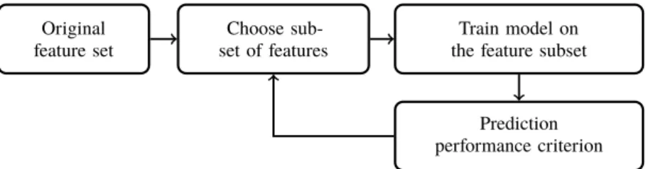
Original feature set

Choose subset of features with the highest metric score

Train model on the feature subset Figure 1:Filters framework.

(4)

2. Wrappers

Wrapper methods are model-based methods for feature selection and are considered to be the most effective and computationally stable algorithms. Figure 2 shows the main principle of the wrapper methods’ framework. Basically, to find the most relevant set of features, the intended model is trained for different subsets of features. The subset with the highest score on a particular performance criterion is selected as best set of features. Because wrapper methods utilize the learning algorithm they are considered more effective and hence more desirable than filters and embedded methods. Original feature set Choose sub-set of features Train model on the feature subset

Prediction performance criterion Figure 2:Wrappers framework.

However, wrapper methods are generally criticized for their excessive computational cost. They require training and evaluation of the perfor-mance of the learning algorithm for every selected subset of features. Fornfeatures, the number of feature subsets is equal toO(2n), i.e., the computational needs of wrappers exponentially increase with the number of features in the model. This makes the search for all possible subsets of features impractical for even moderate values ofn. Sequential search methods such as forward selection, backward elimination and stepwise regression became popular techniques used to overcome some of the computational demands of wrappers. Other efficient search strategies have also been developed to find the desired optimal subset of features (Hocking and Leslie, 1967).

3. Embedded methods

Embedded methods combine the characteristics of filter and wrapper methods. They are implemented by learners that have built-in search procedures for the optimal subset of features (Figure 3). Embedded methods aim at maximizing the performance of the learning algorithm while minimizing the number of features in the algorithm.

(5)

Original feature set Train model on the original feature set

Choose feature subset based on model parameters Figure 3:Embedded methods framework.

Regularization regression methods such as Ridge Regression (Hoerl, 1970), Least Absolute Selection and Shrinkage Operator (LASSO, Tibshirani, 1996) are the most popular forms of embedded methods. Regularized decision tree algorithms, such as random forests (Breiman, 2001), are other examples of embedded methods.

For more comprehensive reviews of feature selection methods, the reader is referred to Guyon and Elisseeff (2003) and Clarke et al (2009).

3 Global Sensitivity Indices

In this section we propose a variance-based feature selection approach for supervised learning in which the variance of the target variables is decomposed into contributions of individual or subsets of features. The technique which was first developed by Sobol (1990, in Russian) and Sobol (1993, in English) relies on the theory of ANOVA decomposition (Efron and Stein, 1981; Scheffé, 1959).

For a model functionY = f(X), the importance of input variables (features) X = (X1, ... ,Xn)is quantified in terms of the reduction in the variance ofY whenXare fixed at some value. For a particular Xi, this is expressed as

Si=

Vi

V(Y) =

VXi[EX−i(Y|Xi)]

V(Y) , i=1,2, ... ,n, (1)

and the joint (interaction) effect is given by

Si j=

Vi j

V(Y) =

V_X_i,Xj[EX−i j(Y|Xi,Xj)] −Vi−Vj

V(Y) , i,j=1,2, ... ,n, i, j, (2)

whereX−i is the set of all variables exceptXiandE(.)andV(.)represent the expected value and variance.Si andSi j represent the first order and interaction effects for Xi and (Xi,Xj), respectively. These effects measure the reduced

(6)

portion of the output (target) variable uncertainty caused by the inputXiand its interactions when the true value ofXi is known. Higher order interaction effects can be defined in a similar fashion. Another popular variance measure of

Xiis the total effect index defined by:

T Si = TVi V(Y) = EX−i[VXi(Y|X−i)] V(Y) =1− VX−i[EXi(Y|X−i)] V(Y) . (3)

T Siis the ratio of the remaining uncertainty of the output to the unconditional varianceV(Y)when the true values of all inputs exceptXiare known. It measures the total effect comprising of first order, interaction and higher order effects involvingXi, i.e., T Si =Si+ n Õ j:j,i Si j+ ... +S1...i...n. (4)

The underlying theory of the above variance-based measures is related to the decomposition of the function f(X)(Sobol, 1993):

f(x)= f0+ n Õ i=1 f_i(X_i)+ Õ 1≤i<j≤n f_{i j}(X_i,X_j)+ ... + f12...n(X1, ... ,Xn) = f₀+ 2n₋₁ Õ s=1 f_I_s(X_I_s), (5) I =1≤i1 < ... <is ≤ n, s =1,2, ... ,2n−1, (6) where f0 =E(Y) (7) fi(Xi)=EX−i(Y|Xi) − f0 (8) fi j(Xi,Xj)=EX−i j(Y|Xi,Xj) − fi− fj− f0 (9) and so on.

(7)

The decomposition in Equation (5) holds true if the model function f(x) is square-integrable and defined over then-dimensional unit hypercube:

Kn= {X|0 ≤ Xi ≤1,i=1, ... ,n} (10) and the integral of every summand over any of its variables is zero, i.e.

1

∫

0

fIs(XIs)dXk =0, k ⊂ I, (11) whereIs is a subset of input variables. For statistically independentX1, ... ,Xn, the terms in Equation (5) are mutually orthogonal and the decomposition is unique. Additionally, with independent inputs, the unconditional varianceV(Y)

can be decomposed in the same way as the model function, i.e.,

V(Y)= n Õ i=1 Vi+ Õ 1≤i<j≤n Vi j+ ... +V12...n (12) with V_i₁_..._i_s =V(f(X_i₁, ... ,X_i_s)) =V[E(f|X_i₁, ... ,X_i_s)], 1≤i1< ... <is ≤n, (13) where the conditional expectation is taken over allXjnot inIsand the variance is computed over the range of possible values ofIs, s=1,2, ... ,2n−1. Dividing both sides of Equation (12) byV(Y), we obtain:

1= n Õ i=1 S_i+ Õ 1≤i<j≤n S_{i j}+ ... .+S₁₂...n (14)

With the identity in Equation (14) and the definitions ofSi andT Si in Equa-tions (1) and (3), it is easy to verify that, if interaction effects exist,

n

Õ

i=1

(8)

and that the difference 1− n Õ i=1 Si (16)

is an indicator of the presence of interaction effects among features. It can also be concluded that

n

Õ

i=1

T Si ≥ 1. (17)

Saltelli et al (2010) suggested that for independent X1, ... ,Xn, one can avoid to explicitly include the probability distribution function of each Xi in the construction of f_i, f_{i j}, ... , etc.Therefore and without loss of generality, all input variables can be conceived as defined inKnand the mapping fromKnto the actual probability distribution ofXiis intended to be part of the definition of fi.

3.1 Monte Carlo Estimation

We construct in this section a Monte Carlo algorithm for the numerical estimation of Sobol sensitivity indices. The Monte Carlo procedure allows the estimation of both sets of indicesSiandT Siusing a single set of random samples generated from the assumed probability distributions ofX. The general framework for the numerical algorithm is as follows:

1. For a given design matrixDof sizeM×nand a vector of output (target) valuesyof sizeM×1, use an appropriate learning algorithm to train the model and obtain predictions f(D). HereMis the number of realizations of features and of the target variable andnis the number of features. 2. For the assumed probability distributions, generate two independent

samplesAandBofX=(X1, ... ,Xn)each of sizeN×n.Nis the number of simulated observations ofX,N ≥ M.

3. For thei-th feature, construct a matrix Ai_B, consisting of all columns of

Aexcept thei-th column which is taken from matrixB.

4. EstimateViandTVi, the numerators ofSiandT Siin Equations (1) and (3), respectively, andV(Y)by the following formulas (Saltelli et al, 2010):

ˆ Vi = 1 N N Õ r=1 f(B)_r[f(A_Bi )_r − f(A)_r] (18)

(9)

ˆ TVi = 1 2N N Õ r=1 [f(Ai_B)r − f(A)r]2 (19) ˆ V(Y)= 1 N N Õ r=1 f(A)_rf(B)_r − f₀2 (20)

wherer is therth row ofAandBand

f0 = 1 N N Õ r=1 f(A)r. (21)

5. Use Equations (1) and (3) to obtain the estimated values for first-order and total effect indices, ˆSiand ˆT Si.

6. For a givenk, select the features with the highestk% first-order or total effect scores.kdepends on the desired accuracy of the model.

The number of model evaluations required by the above estimation algorithm for the combined set of ˆSi and ˆT Si is N(n+2). A larger N produces more accurate estimates. Another important aspect of the computation is the random sampling of the two matrices Aand B. The Monte Carlo method makes use of quasi-random (QR) points of the Sobol sequences (Bratley and Fox, 1988). QR sequences possess the desired uniformity property and optimally fill the unit hypercubeKnin a fashion that avoids inhomogeneity of selected points. Sobol sequences possess the additional favored property of being low discrepancy points and they perform well in existing QR methods. More details about the characteristics and generation of Sobol QR sequences can be found in Saltelli et al (2010).

4 Numerical Example

The above described computational algorithm of Sobol sensitivity indices is ap-plied here to a published data set containing 100 independent variables (features) and one output (target) variable (source:https://drive.google.com/ file/d/0ByPBn4rtMQ5HaVFITnBObXdtVUU/view). The features rep-resent various profiles of certain stocks while the target variable reprep-resents a rise in the stock price (1) or a drop in stock price (−1).

(10)

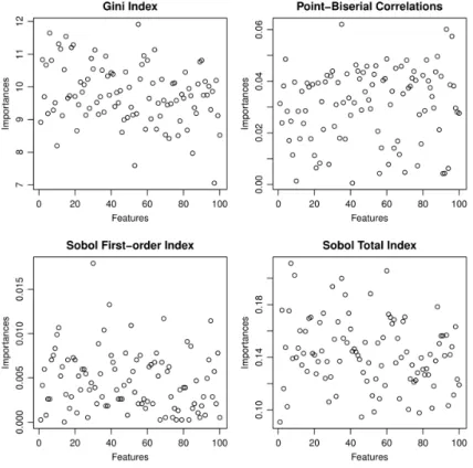
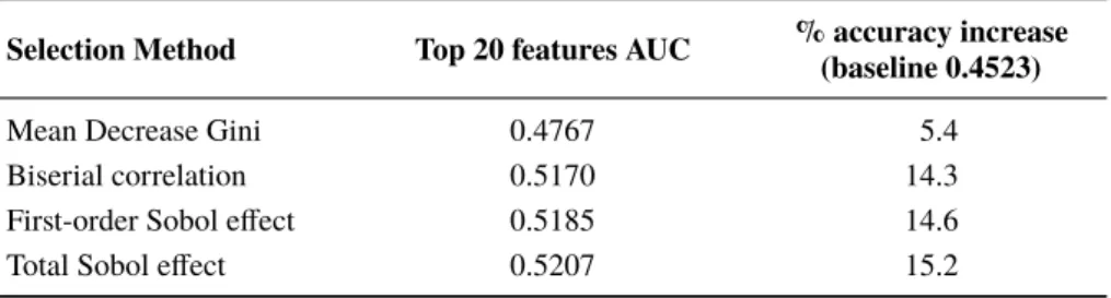
The data set includes 3000 observations. The model was first trained by a Random Forest (RF) utilizing 67 % of the data set and the model was validated on the remaining 33 % of the observations. The reported accuracy of the validated model – measured by the Area Under Curve (AUC) – was 0.4523. Using the mean decrease in the Gini index measure for feature importance (Clarke et al, 2009), the top 20 features were selected and the model was retrained with these most important 20 features. The resulting validated prediction accuracy was 0.4767 (5.4 % increase in accuracy). We followed the same learning algorithm and applied instead the global sensitivity analysis to select the top 20 features. We usedN =15000 simulations. A filter method based on the point-biserial correlation coefficient of each feature with the binary target variable is added to the analysis. The results are shown in the following Figure 4 and Table 1.

(11)

Figure 4 depicts scatter plots of the feature relevance (importance) values computed based on mean decrease in the Gini index (as reported in the source article), point-biserial correlation coefficient and Sobol sensitivity indices versus feature index. A quick examination of the scatter plots reveals that the first-order Sobol sensitivity indexS_ihas the strongest discrimination ability of the most important features, followed by biserial correlation and total sensitivity index

T Si. The three measures possess more dispersed scatters in the upper range as compared to the Gini index.This is confirmed by the values of the coefficient of variation which are from highest to lowest: 73 % forSi, 45 % for biserial correlation, 37 % forT Siand 9 % for Gini index.

Table 1:Prediction accuracy of reduced model.

Selection Method Top 20 features AUC % accuracy increase

(baseline 0.4523)

Mean Decrease Gini 0.4767 5.4

Biserial correlation 0.5170 14.3

First-order Sobol effect 0.5185 14.6

Total Sobol effect 0.5207 15.2

Table 1 clearly indicates that the Sobol sensitivity indices produce the highest predictive accuracy when the model is trained on the top 20 selected features.

5 Conclusion

In this paper a supervised feature selection approach is proposed based on the global sensitivity analysis. Feature importance is measured by the first-order and total Sobol sensitivity indices that quantify the contribution of individual features and their interactions to the overall variance of the target variable. A computational algorithm of the two sensitivity indices was described and applied to a publicly available data set. It is shown that Sobol sensitivity indices identify the most important features more distinctly than other existing feature selection techniques and provide a higher predictive accuracy.

(12)

The classical Sobol-based sensitivity analysis presented in this paper assumes statistically independent features. In subsequent work, the authors wish to extend the analysis to include dependent features and also compute sensitivity indices for subsets of features.

Acknowledgements The authors gratefully acknowledge the support of the American University of Sharjah, United Arab Emirates.

References

Aliferis C, Statnikov A, Tsamardinos I, Mani S, Koutsoukos X (2010) Local causal and Markov Blanket induction for causal discovery and feature selection for classification. Journal of Machine Learning Research 11:171–234.

Bratley P, Fox B (1988) Sobol’s quasirandom sequence generator. Association for Computing Machinery Transactions on Mathematical Software 14:88–100. Breiman L (2001) Random forests. Machine Learning 45(1):5–32, Kluwer Academic

Publishers. DOI: 10.1023/A:1010933404324.

Clarke B, Fokoué E, Zhang H (2009) Principles and theory for data mining and machine learning, 1st edn. Springer, New York. DOI: 10.1007/978-0-387-98135-2.

Efron B, Stein C (1981) The Jackknife estimate of variance. The Annals of Statistics 9(3):586–596.

Guyon I, Elisseeff A (2003) An introduction to variable and feature selection. Journal of Machine Learning Research 3:1157–1182.

Hocking R, Leslie R (1967) Selection of the best subset in regression analysis. Tech-nometrics 9:531–540.

Hoerl R A.E.and Kennard (1970) Ridge regression: biased estimation for nonorthogonal problems. Technometrics 12:55–67.

Janecek A, Gansterer W, Demel M, Ecker G (2008) On the relationship between feature selection and classification accuracy. Proceedings of the Workshop on New Challenges for Feature Selection in Data Mining and Knowledge Discovery at ECML/PKDD 2008, Proceedings of Machine Learning Research (PMLR) 4:90–105. Maio J, Niu L (1981) A Survey on Feature Selection. DOI: 10.1016/j.procs.2016.07.111. Saltelli A, Annoni P, Azzini I, Campolongo F, Ratto M, Tarantola S (2010) Variance based sensitivity analysis of model output. Design and estimator for the total sensitivity index. Computer Physics Communications 181(2):259–270. DOI: 10.1016/j.cpc.2009.09.018.

(13)

Scheffé H (1959) The analysis of variance. Wiley series in probability and mathematical statistics. Probability and mathematical statistics, John Wiley & Sons, New York. Sobol I (1990) On sensitivity estimation for nonlinear mathematical models (in Russian).

Matematicheskoe Modelirovanie 2:112–118.

Sobol I (1993) Sensitivity estimates for nonlinear mathematical models. Mathematical Modeling and Computational Experiment 1:407–414.

Tibshirani R (1996) Regression shrinkage and selection via the lasso. Journal of the Royal Statistical Society, Series B (Methodological) 58(1):267–288.