A mobile network planning tool based on data analytics

(1)

Research Article

A Mobile Network Planning Tool Based on Data Analytics

Jessica Moysen, Lorenza Giupponi, and Josep Mangues-Bafalluy

Centre Tecnol`ogic de Telecomunicacions de Catalunya (CTTC), Av. Carl Friedrich Gauss 7, 08860 Castelldefels, Spain Correspondence should be addressed to Jessica Moysen; [email protected]

Received 3 August 2016; Accepted 14 November 2016; Published 5 February 2017 Academic Editor: Piotr Zwierzykowski

Copyright © 2017 Jessica Moysen et al. This is an open access article distributed under the Creative Commons Attribution License, which permits unrestricted use, distribution, and reproduction in any medium, provided the original work is properly cited. Planning future mobile networks entails multiple challenges due to the high complexity of the network to be managed. Beyond 4G and 5G networks are expected to be characterized by a high densification of nodes and heterogeneity of layers, applications, and Radio Access Technologies (RAT). In this context, a network planning tool capable of dealing with this complexity is highly convenient. The objective is to exploit the information produced by and already available in the network to properly deploy, configure, and optimise network nodes. This work presents such a smart network planning tool that exploits Machine Learning (ML) techniques. The proposed approach is able to predict the Quality of Service (QoS) experienced by the users based on the measurement history of the network. We select Physical Resource Block (PRB) per Megabit (Mb) as our main QoS indicator to optimise, since minimizing this metric allows offering the same service to users by consuming less resources, so, being more cost-effective. Two cases of study are considered in order to evaluate the performance of the proposed scheme, one to smartly plan the small cell deployment in a dense indoor scenario and a second one to timely face a detected fault in a macrocell network.

1. Introduction

Nowadays, we are assisting to the definition of what 5G networks will look like. 3GPP has started multiple work items that will lead to the definition of a novel 5G radio and architecture [1]. The main vendors are publishing numer-ous white papers presenting their view on 5G networks and architectures. The EU commission has put in place an important 5G Infrastructure Public Private Partnership (5GPPP) program to fund research for5G networks [2]. What is clear from all these converging visions is that network management in beyond4G and future5G networks has to face a whole new set of challenges, due to (1) ultradense deployments, heterogeneous nodes, networks, applications, and Radio Access Networks (RANs) and also heterogeneous spectrum access through novel technologies, such as Long Term Evolution Unlicensed (LTE-U) and License Assisted Access (LAA), all coexisting in the same setting, (2) the need to manage very dynamic networks where part of the nodes is controlled directly by the users (e.g., femtocells), energy saving policies generating a fluctuating number of nodes, active antennas, and so on, (3) the need to support 1000x traffic and 10x users and to improve energy efficiency, (4) the

need to improve the experience of the users by enabling Gbps speeds and highly reduced latency, or (5) the need to manage new virtualised architectures.

In this context, it is already widely recognized that the network needs to establish new procedures to become more intelligent, self-aware, and self-adaptive. An initial step in this direction has been introduced in 4G LTE networks, since Release 8, with the introduction of Self-Organising Network (SON). However, this vision needs to be further developed in 5G considering the huge complexity of these networks. As we already observed in [3], a huge amount of data is currently already generated in 4G networks during normal operations by control and management functions, and more data is expected to be gathered in 5G networks due to the densification process [4], heterogeneity in layers and technologies, the additional control and management complexity in Network Functions Virtualisation (NFV) and Software Defined Network (SDN) architectures, the increas-ing relevance of Machine to Machine (M2M) and Internet of Things (IoT) communications, the increasing variety of applications and services, each with distinct traffic patterns and QoS/Quality of Experience (QoE) requirements, and so on.

Volume 2017, Article ID 6740585, 16 pages https://doi.org/10.1155/2017/6740585

(2)

The main objective of network management is then to make the network (1) more self-aware, by exploiting and analysing data already generated by the network (this is expected to drive network management from reactive to pre-dictive) and (2) more self-adaptive by exploiting intelligent control decisions tools, offered by ML, based on learning and experience.

In this paper, among many network management prob-lems, we focus on smart network planning, which gives particular emphasis to the QoS offered to the users and the resources used by the operator to offer it. We believe that the use of smart network planning tools is crucial and inevitable for operators running multi-RAT, multivendor, multilayer networks, where an overwhelming number of parameters needs to be configured to optimise the network performance. The state of the art in network planning, in literature, and in the market offers a wide range of platforms systems and applications proposed by the research community and/or oriented to the industry. From an industry perspective, the market of commercial planning tools aims at providing a complete set of solutions to design and analyse networks [5–8]. For instance, in [9], the authors present an open-source network planning tool that includes different planning algorithms to analyse the network under different failures and energy efficiency schemes. However, these works in general focus on several configuration scenarios, RF coverage planning, network recovery test, traffic load analysis, and forecasting traffic, among others, and not directly on QoS offered to end-users and the resources that mobile network operators need to offer. Other works are more targeted to QoS estimation, but not in the area of network planning. The literature already offers different works targeting the problem of QoS prediction and verification, such as [10, 11]. In our preliminary work [12], we focus on complex multilayer heterogeneous networks where we predict QoS indepen-dently of the physical location of the UE, that is, based on data learned throughout the whole network. Preliminary results show that by abstracting from the physical position of the measurements we can provide high accuracies in the estimations of QoS in other arbitrary regions. Furthermore, the results presented in [13] show that data analysis achieves better performance in a reduced space rather than in the original one.

This paper presents a smart network planning tool that works in two steps. First, it estimates the QoS at every point of the network based on user-collected measurements, which may have been taken at different time instants and anywhere in the heterogeneous network. We perform this estimation through supervised learning tools. This results in an appropriately tuned QoS prediction model, which is then integrated in the next step. Second, we adjust the network parameters in order to reach certain network objectives by evaluating different combinations and calculating the result-ing QoS based on the model of step 1. Network objectives are set in terms of PRB per Mb. We focus on this specific QoS indicator because it combines information that is relevant to the operator (PRBs) and other that is relevant to the end-user (Mb of data) into a single metric. Therefore, the minimization of this indicator allows serving users with an improved

spectral efficiency and offered QoS. More specifically, to carry out this optimisation we take advantage of GAs, which are stochastic search algorithms useful to implement learning and optimisation tasks [14], and so are adequate for our purpose.

In order to evaluate the performance of the proposed scheme, we consider two use cases. The first one is in a densified indoor scenario, and the second one is in a more traditional macrocell scenario. In the first use case, we focus on how to plan a dense small cell deployment inspired in a typical 3GPP dual stripe scenario [15], where the parameters to adjust are the number of small cells and their position. In the second use case, we deal with self-healing aspects in macrocellular scenarios. We focus on readjusting the parameters of the surrounding cells to quickly solve an outage problem by automatically adjusting their antenna tilt parameters.

We evaluate the performance of the proposed planning tool through a network simulation campaign carried out over the 3GPP compliant, full protocol stack ns-3 LENA module. We show that the proposed ML-based network plan-ning, differently from other closed optimisation approaches, is extremely flexible in terms of application problem and scenario, and, in this sense, it is generic. Without loss of gen-erality, particular attention has been focused on how to plan a dense 4G small cell deployment and how to quickly solve an outage problem. As can be seen, the approach is equally valid and shows good performance in both studied use cases, characterized by very different optimisation problems and scenarios. As for the RAT, we have focused on 4G and its evolution. The same technique can be applied also to 2G and 3G technologies.

This paper is organised as follows. The general approach is described in Section 2. It describes the ML-based network planning tool, its main design principles, and algorithms we use to build it. In Section 3, we discuss the specific design details and tuning of the QoS prediction model and we put all the pieces (i.e., prediction and optimisation) together. In Section 4, we present the details of the two use cases to which the tool is applied, the simulation platform, and the simulations results. Finally, Section 5 concludes the paper.

2. ML-Based Network Planning

Tool Description

We propose designing a network planning tool, which works in two steps. First, we propose to model the QoS through the analysis of data extracted from the networks in the form of measurements. This phase requires to first prepare the data and then to analyse it. And second, we keep on adjusting the parameters and analysing the impact on QoS based on the previous model. In this way, the performance of the network is optimised to meet certain operator targets. Figure 1 presents the different phases required by the proposed network plan-ning.

(1) Data Preparation.This process aims at transforming data into a meaningful format for the estimation at hand. The target is to integrate and prepare large volumes of data

(3)

Table 1: Relevant sources of information in mobile networks.

Source Information Usage

Control info for short-term network operation

Call/session setup, release, maintenance QoS, RRC, idle and connects mode mobility

Discarded after usage Control info for SON

functions

Info on Radio link failure, intercell interference, UE measurements, MDT measurements, radio resource

status, cell load signalling, etc.

Heuristic algorithms typically discard info

after

Management information for long-term operation

Fault configuration, accounting, performance and security management (FCAPS), Operations and Management, e.g.,

in OAM aggregated statistics per eNB, on network performances, # users, successful/failed HO, active

bearers, information from active probing

Mainly used for triggering engineer

intervention Customer Relationship

Information Complaints about bad service quality, churn info

Only used by customer service

Data preparation Data analysis Optimised network

planning

(i) Reducing the high dimensional space (ii) Building machine learning models Modelling QoS

(i) Collecting the data

(iii) Loading the data (ii) Preprocessing the

data

(i) Optimisation of decision making process

Figure 1: Architecture of the network planning tool.

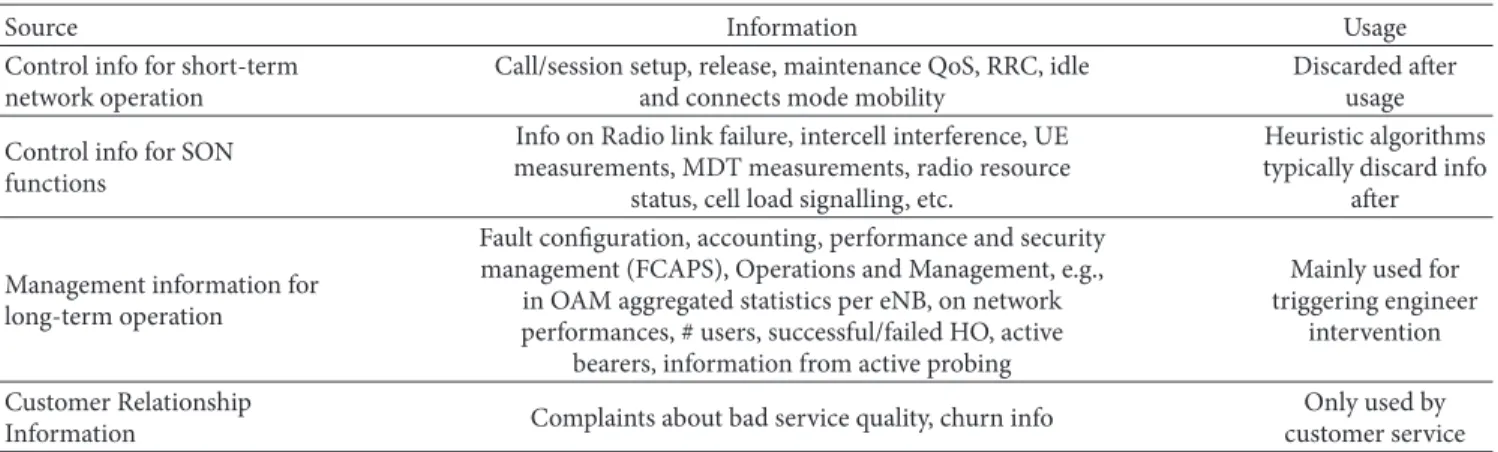
over the network to provide a unified information base for analysis. To do this, we follow the Extract-Transform-Load (ETL) process, which is responsible for pulling data out of the source and placing it into a database. It involves 3 main steps: data extraction (E), whose objective is to collect the data from different sources; data transformation (T), which prepares the data for the purpose of querying and analysis; data loading (L), which loads the data into the main target, most of the cases into a flat file. This process plays an important role for the design and implementation of planning for future mobile networks. The objective is to create a data structure that is able to provide meaningful insights. Some examples of the kind of sources available in mobile networks are shown in Table 1 [3]. Here the data are classified based on the purpose for which they are generated in the network. The usage that is given nowadays in the network is also suggested in the last column. For the purpose of network planning, we plan to extract data reported by the UEs to the network in the form of UE measurements, in terms of received power, received quality, and offered QoS.

Once the data has been collected, we prepare the data for storing, using the proper structure for the querying.

(2) Data Analysis.The objective of this process is to discover patterns in data that can lead to predictions about the future. This is done by finding this information/correlation among the radio measurements extracted from the network. We do this by applying ML techniques.

(3) Optimised Network Planning.The objective of this process is to find the configuration parameters for the optimised

network planning based on the information extracted from the previous data analysis process. In the complex cellular context, we need to deal with several network characteristics that introduce high complexity, for example, the very large number of parameters, the strong cross-tier interference, fast fading, shadowing, and mobility of users. In order to deal with these issues and to guarantee an appropriate network planning, in this work, we propose to use GAs, which allow avoiding some of the problems of typical closed optimisation techniques (e.g., computational intractability) in this complex and dynamic scenario. More specifically, they work with chromosomes (i.e., a given combination of values for the parameters to be tuned in the network). For each of the chromosomes, they calculate its fitness score based on a given objective function (in our case, the QoS predicted by the model) [17]. Then, they select the chromosomes with the best fitness score and generate better child chromosomes by combining the selected ones and they keep on iterating until the objective function of the chromosomes generated reaches the performance target. In this way, GAs perform parallel search from a population of points, which represent the values of the different parameters to be tuned in the scenario and, jointly with other techniques, they have the ability to avoid local minima and use probabilistic search rules.

2.1. Modelling the QoS. We estimate the QoS at every point of the network based on measurements collected in different moments in time and from other regions of the heteroge-neous network, that is, based on the measurement history of the network. To do this, we consider thedata preparation

and data analysis processes of the network planning tool. As mentioned previously, the objective of these 2 processes is to extract, prepare, and analyse the information already available in the network to provide insightful information from the analysis of it. In fact, in this kind of estimations, ML techniques can be very effective to make predictions based on observations. Therefore, we take advantage of ML techniques to create a model that allows estimating the QoS by learning the relation between PHY layer measurements and QoS measured at the UE. We propose using SL, since among many applications it offers tools for estimation and

(4)

prediction of behaviours. In particular, we focus on a regres-sion problem, since we want to analyse the relationship between a continuous variable (PRB per Mb) and the data extracted from the network in the form of UE measurements. Many regression techniques have been developed in the SL literature, and criteria to select the most appropriate method include aspects such as the kind of relation that exists between the input and the output or between the considered features, the complexity, the dimension of the dataset, the ability to separate the information from the noise, the training speed, the prediction speed, the accuracy in the prediction, and so on. We focus on regression models, and we select the most representative approaches. We then use ensemble methods to sub-sample the training samples, prioritizing criteria such as the low complexity and the high accuracy.

We then build a dataset of user measurements, based on the same data contained in the Minimization of Drive Tests (MDT) database. The MDT is a standardized database used for different 3GPP use cases. The dataset contains training samples (rows) and features (columns) and is divided into 2 sets, the training set to train the model and the test set to make sure that the predictions are correct. That training data develop a predictive model and evaluate the accuracy of the prediction, by inferring a function 𝑓(x), returning the predicted output ̂𝑦. The input space is represented by an𝑛-dimensional input vectorx = (𝑥(1), . . . , 𝑥(𝑛))𝑇 ∈ R𝑛. Each dimension is an input variable. In addition, a training set involves𝑚training samples((x₁, 𝑦₁), . . . , (x_𝑚, 𝑦_𝑚)). Each sample consists of an input vector x_𝑖 and a corresponding output𝑦_𝑖of one data point𝑖. Hence,𝑥(𝑗)_𝑖 is the value of the input variable𝑥(𝑗)in training sample𝑖, and the error is usually computed via|𝑦_𝑖− ̂𝑦_𝑖|or with the root mean square error.

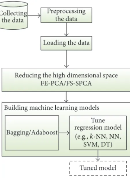
In addition to regression analysis, we exploit Unsuper-vised Learning (UL) techniques for dimensionality reduction to filter the information in the data that is actually of interest (thus reducing the computational complexity) while maintaining the prediction accuracy. We do this by feeding the data into an ensemble method consisting of Bagging/ AdaBoost to manipulate the training samples. And after that, the SL techniques under evaluation are then applied. Details for each step are given in the following, and the whole process is depicted in Figure 2.

(1) Collecting the Data.The data we take into account comes from mobile networks, which generate data in the form of network measurements, control, and management informa-tion (Table 1). As we meninforma-tioned previously, we focus on MDT functionality, which enables operators to collect User Equipment (UE) measurements together with location infor-mation, if available, to be used for network management, while reducing operational costs. This feature has been intro-duced by 3GPP since Release 10; among the targets there are the standardization of solutions for coverage optimisation, mobility, capacity optimisation, parametrization of common channels, and QoS verification. In this context, the literature already offers different solutions for this feature. An example of that can be observed in, [18, 19]. Since operators are also interested in estimating QoS performance, in Release 11, the

Building machine learning models Reducing the high dimensional space

FE-PCA/FS-SPCA Bagging/Adaboost Tuned model Preprocessing the data Collecting the data

Loading the data

Tune regression model

SVM, DT)

(e.g.,_k-NN, NN,

Figure 2: Modelling the QoS.

MDT functionality has been enhanced to properly dimension and plan the network by collecting measurements of through-put and connectivity issues [20]. Therefore, we collect for each UE (1) the Reference Signal Received Power (RSRP) and (2) the Reference Signal Received Quality (RSRQ) coming from the serving and neighbouring eNBs. The size of the input space is[𝑙 × 𝑛]. The number of rows is the number𝑙of UE in the scenario, and the number of columns corresponds to the number of measurements𝑛. The size of the output space is [𝑙×1], which corresponds to the QoS performance in terms of the PRB per transmitted Mb. These measurements gathered at arbitrary points of the network throughout its lifetime are exploited to plan other arbitrary future deployments.

(2) Preprocessing the Data. In order to obtain a good per-formance during the evaluation, the input variables of the different measurements must be in a similar scale and range. So, a common practice is to normalize every variable between −1 ≤ 𝑥(𝑗)_{≤ 1}_{range and replace}_𝑥(𝑗)_with_𝑥(𝑗)_{− 𝜇}(𝑗)_{, over the}

difference between the maximum and minimum values of the input variables in the dataset, where𝜇(𝑗)is the average of the input variable(𝑗)in the dataset. The normalized data is then split into training and test set. We create a random partition from the𝑙sets of input. This partition divides the observations into a training set of𝑚samples and a test set𝑝 = 𝑙 − 𝑚 samples. We randomly select approximately𝑝 = (1/5) × 𝑙 observations for the test set.

(3) Loading the Data. This process varies widely. As we mentioned before, depending on the operator requirements, the data can be updated or new data can be added in a historical form at regular intervals. For our propose, in this particular work, we maintain a history of all changes to the data loaded in the network.

(4) Reducing the High Dimensional Space.One of the prob-lems that mobile operators have to face in this kind of

(5)

networks is the huge amount of potential features we have as input. In our particular case, features would substantially increase as networks densify. Therefore, to deal with the huge amount of features, we propose applying regression techniques in a reduced space, rather than in the original one. The idea behind that comes from our previous work [12], in which we observed that using a high dimensional space did not result in the best performance. Therefore, we suggest applying the regression analysis in a reduced space. As a result, we take advantage of dimensionality reduction techniques to reduce the number of random variables under consideration. These methods can be divided into Feature Extraction (FE) and Feature Selection (FS) methods. Both methods seek to reduce the number of features in the dataset. FE methods do so by creating new combinations of features (e.g., Principal Component Analysis (PCA)), which project the data onto a lower dimensional subspace by identifying correlated features in the data distribution. They retain the 𝑐 Principal Components (PCs) with greatest variance and discard all others to preserve maximum information and retain minimal redundancy [21]. Correlation-based FS meth-ods include and exclude features present in the data without changing them. An example is Sparse Principal Component Analysis (SPCA), which extends the classic method of PCA for the reduction of dimensionality of data by adding sparsity constraints on the input features; that is, by adjusting a set of weights over the input features, it induces a matrix in which most of the elements are zero in the solution. In FS-SPCA the sparsity is used to select the𝑓features that give the most useful information; as we increase the weight of SPCA, the number of features is reduced. That is, by adding sparsity constraints on the input features, we promote solutions in which only a small number of input features capture most of the variance. Some preliminary work on these features was presented in [13].

(5) Building the Machine Learning Models.We select some representative regression models, prioritizing criteria such as low complexity and high accuracy: (1)𝑘-Nearest Neighbours (𝑘-NN), (2) Neural Networks (NN), (3) Support Vector Machines (SVMs), and (4) Decision Tree (DT), and we analyse them by performing an empirical comparison of these algorithms, observing the impact on the prediction of the different kinds and amounts of UE measurements.

(1)𝑘-NN can be used for classification and regression [22]. The𝑘-NN method has the advantage of being easy to interpret and fast in training and parameter tuning is minimal.

(2) NN is a statistical learning model inspired by the structure of a human brain where the interconnected nodes represent the neurons to produce appropriate responses. NN support both classification and regres-sion algorithms. NN methods require parameters or distribution models derived from the dataset, and in general they are susceptible to overfitting [23]. (3) SVMs can be used for classification and regression.

The estimation accuracy of this method depends on a good setting of the regularization parameter𝐶,𝜖,

and the kernel parameters. This method in general shows high accuracy in the prediction, and it can also behave very well with nonlinear problems when using appropriate kernel methods [24].

(4) DT is a flow-chart model, which supports both clas-sification and regression algorithms. Decision trees do not require any prior knowledge of the data, are robust, and work well on noisy data. However, they are dependent on the coverage of the training data, as is the case for many classifiers, and they are also susceptible to overfitting [25, 26].

In order to enhance the performance of each learning algorithm described before, instead of using the same dataset to train, we can use multiple data sets by building an ensemble method. Ensemble methods are learning models that combine the opinions of multiple learners. This tech-nique has been investigated in a huge variety of works [27, 28], where the most useful techniques have been found to be Bagging and AdaBoost [29]. Bagging manipulates the training examples to generate multiple hypothesis. It runs the learning algorithm𝑛itertimes, each one with a different

subset of training samples. AdaBoost works similarly, but it maintains a set of weights over the original training set and adjusts these weights by increasing the weight of samples that are misclassified and decreasing the weight of examples that are correctly classified [30].

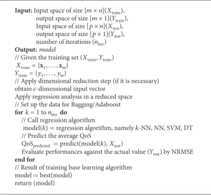
In summary, once the extracted data has been processed and loaded into a file, it is fed into a dimensionality reduc-tion step, and subsequently into an ensemble step, which manipulates the training set by applying Bagging/AdaBoost techniques. The learning algorithm is then applied to produce a regression (see Algorithm 1).

(6) Evaluation of Accuracy.To evaluate the accuracy of the model, the performance of the learned function is measured on the test set. That is, we use a set of samples used to tune the regression algorithm. For each test value, we predict the average QoS and compare it with the actual value in terms of the Root Mean Squared Error (RMSE) of the prediction as follows RMSE= √∑𝑝_𝑖=1(𝑦_𝑖− ̂𝑦_𝑖)2/𝑝, where𝑝is the length of the test set,̂𝑦_𝑖indicates the predicted value, and𝑦_𝑖is the testing value of one data point𝑖. In order to compare the RMSE with different scales, the input and output variable values are normalized as follows: NRMSE = RMSE/(𝑦_max− 𝑦_min), where𝑦_maxand𝑦_minrepresent the max and min values in the output space𝑌testof size[𝑝 × 1], respectively.

2.2. Optimised Network Planning. As we mentioned before, the objective of this process is to close the loop by adjusting the parameters, and so the network performance, through a GA. This results in a GA organised into different phases, as depicted in Figure 3.

(1) Create S Feasible Solutions. We create a set S =

{𝜃(1), . . . ,𝜃(𝑝size)} _{of feasible solutions (also called}

chromo-somes or individuals), where𝑝sizeis the starting population

(6)

Input:Input space of size[𝑚 × 𝑛](𝑋_train), output space of size[𝑚 × 1](𝑌train), Input space of size[𝑝 × 𝑛](𝑋test), output space of size[𝑝 × 1](𝑌_test), number of iterations (𝑛_iter)

Output:𝑚𝑜𝑑𝑒𝑙

// Given the training set (𝑋_train, 𝑌_train)

𝑋train= {x1, . . . ,x𝑚}

𝑌train= {𝑦1, . . . , 𝑦𝑚}

// Apply dimensional reduction step (if it is necessary) obtain𝑐-dimensional input vector

Apply regression analysis in a reduced space // Set up the data for Bagging/Adaboost

for𝑘 = 1to𝑛_iter do

// Call regression algorithm

model(𝑘)flregression algorithm, namely𝑘-NN, NN, SVM, DT // Predict the average QoS

QoSpredicted flpredict(model(𝑘),𝑋test)

Evaluate performances against the actual value (𝑌_test) by NRMSE

end for

// Result of training base learning algorithm modelflbest(model)

return (model)

Algorithm 1: Train regression algorithm.

Evaluate network deployment performance Selection Crossover Mutation yes no Output Desired performance reached? Create S random initial feasible solutions

Figure 3: Optimised network planning.

parameters vector of an individual𝑠, with𝜃(𝑠)_𝑗 denoting the value for the parameter of eNB𝑗, for instance, the transmitted power (𝜃(𝑠)_𝑗

txp), the antenna tilt (𝜃

(𝑠)

𝑗tilt), or the action to switch ON

or OFF (𝜃(𝑠)_𝑗_sc) the𝑗th small cell.

(2) Evaluate Network Deployment Performance.This function is responsible for evaluating the network deployment perfor-mance. The objective is to calculate the objective function (fitness) of each individual. Given a particular configuration parameter vector𝜃(𝑠), this function is responsible for return-ing the average offered QoS, that is, the average network per-formance predicted based on the measurement history of the network. This function takes as inputSfeasible solutions and the model produced by the regression algorithm discussed in the previous section. That is, the output of Algorithm 1.

The behaviour of this module is as follows. In each iteration, we collect𝑋evalmeasurements in some arbitrary𝑞

points in the scenario. These measurements are obtained as a consequence of having configured the parameters of the sce-nario according to each𝜃∈S. Based on these measurements, the QoS in the points of interest is predicted by using the model generated in step 1 (seeevalNetPerformancefunction in Algorithm 2). Finally, for a given individual, the average of the predicted QoS at the𝑞points is returned as an indicator of the performance of the system with this setup.

As we mentioned before, our metric of interest is the PRB per transmitted Mb, since reducing it allows improving the QoS of the users while also improving the spectral efficiency of the operator. Therefore, the fitness function aims at finding the configuration of parameters for which the total PRB per transmitted Mb is minimized. The operator can target a desired value for the total PRB per transmitted Mb, and, based on this, the network planning tool can decide when the objective has been achieved and interrupt the operation. Therefore, as in any GA, we try to improve the tuning of parameters for each new generation through the processes

(7)

Input:Configuration parameters vector (𝜃), the tuned model (model)

Output:average QoS

evalNetPerformanceflfunction(𝜃, model){

// Call ns-3 network simulator evaluate𝜃(s)= (𝜃₁(𝑠), . . . , 𝜃_𝑀(𝑠))

// Collect measurements at𝑞points in the scenario

𝑋eval= {x1, . . . ,x𝑞}

// Predict the average QoS

QoSpredictedflpredict(model,𝑋eval)

average QoSflmean(QoS_predicted) return (average QoS)}

Algorithm 2: Evaluate network deployment performance.

described below (i.e., selection, crossover, and mutation). And our measure of improvement is the average predicted QoS values for the individuals belonging to each generation.

(3) Selection.We select the best fit individuals for reproduc-tion based on their fitness, that is, this funcreproduc-tion generates a new population of individuals from the current population. This selection is known as elitist selection. Elitism copies the best𝑒fittest candidates into the next generation.

(4) Crossover. This function forms a new individual by combining part of the genetic information from their parents. The idea behind crossover is that the new individual may be better than both parents if he takes the best characteristics from each of them. We use an arithmetic crossover, which creates new individuals (𝛽) that are the weighted arithmetic mean of two parents. If 𝜃(𝑎) and 𝜃(𝑏) are the parents, the function returns as follows:

𝛽 = 𝛼 ×𝜃(𝑎)+ (1 − 𝛼) ×𝜃(𝑏), (1) where 𝛼 is a random weighting factor chosen before each crossover operation. That is, the arithmetic crossover oper-ator combines two parent chromosome vectors to produce a new individual, where𝛼is a random value between[0, 1].

(5) Mutation. This function randomly selects a parameter based on a uniform random value between a minimum and maximum value. It maintains the diversity in the value of the parameters for subsequent generations. That is, it avoids premature convergence on a local maximum or minimum. For that, we set to𝛿the probability of mutation in a feasible solution 𝜃(𝑠). If 𝛿 is too high, the convergence is slow or it never happens. Therefore, most of the times 𝛿 tends to be small. Finally, we replace the worst fit population with new individuals. The whole genetic algorithm is described in Algorithm 3.

3. Design of the Network Planning Tool

This section presents a discussion on how to tune the model for the ultradense complex scenarios under consideration

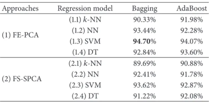
Table 2: Overall model accuracy.

Approaches Regression model Bagging AdaBoost

(1) FE-PCA (1.1)𝑘-NN 90.33% 91.98% (1.2) NN 93.44% 92.28% (1.3) SVM 94.70% 94.07% (1.4) DT 92.84% 93.60% (2) FS-SPCA (2.1)𝑘-NN 89.69% 90.88% (2.2) NN 92.41% 91.78% (2.3) SVM 93.62% 92.87% (2.4) DT 91.22% 92.08%

and then explains how this model is integrated into the global network planning tool.

3.1. Design and Evaluation of the QoS Modelling Component.

This section compares the different options for each of the components that define our QoS model, namely, dimension-ality reduction, ensemble methods, and regression methods. We consider different options for each of them: (1) FE-PCA and FS-SPCA for dimensionality reduction; (2) Bagging and AdaBoost as ensemble methods; and (3)𝑘-NN, NN, SV, and DT as regression models, as anticipated in Section 2.1.

Table 2 summarizes the performance accuracy of each learning algorithm. Accuracy is measured as(1 −NRMSE) × 100. Based on this table, we discuss potential design deci-sions:

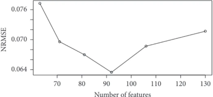
(1) FS-SPCA is a very useful approach if we are interested in excluding features to retain minimal information redundancy. This can be observed in Figure 4, which shows the NRMSE as a function of different number of features (𝑓) selected by the SPCA, and where results reveal that for𝑓 = 92features we obtain the lowest NRMSE value. As a consequence, we select the 92features that give us the most useful information. On the other hand, for the FE-PCA approach, we observed in Figures 5 and 6 that we can obtain the 70% of cumulative variance if we consider 𝑐 = 10 PCs. That is, with the first10PCs we already capture the main variability of the data. Therefore, on the one hand, FE-PCA would present less inputs to the SL step of the data processing chain at the cost of a prior processing of features. On the other hand, FS-SPCA would simplify the initial feature processing, since selected features are taken as they are, but the cost would be the higher needed storage.

In terms of the overall accuracy of the prediction, by implementing the FS-SPCA approach, we can reduce the dimensionality of the data down to𝑓features and still maintain almost the same accuracy with respect to FE-PCA approach. That is, if we consider the 92 features, we lose only1% of accuracy with respect to FE-PCA (i.e., 92 inputs versus 10 inputs to the SL step). Therefore, it will depend on the specific network and operator to select whether computing or storage

(8)

Input:Initial population (S), size ofS(𝑝_size),

the tuned model (model), number of generations (𝑔), rate of elitism𝑒, rate of mutation𝛿 Output:solution𝜃(∗) //Initialization for𝑖 = 1to𝑔do

// Return the value of average QoS describing the fitness of each individual𝜃∈S

for all𝜃∈S do

average QoSfl evalNetPerformance(𝜃, model)

end for

// Elitism based selection select the best𝑒solutions // Crossover

number of crossover𝑛_𝑐= (𝑝_size− 𝑒)/2

for𝑗 = 1to𝑛_𝑐do

randomly select two solutions𝜃(𝑎)and𝜃(𝑏) generate𝜃(𝑐)by arithmetic crossover to𝜃(𝑎)and𝜃(𝑏)

end for

// Mutation

for𝑗 = 1to𝑛_𝑐do

mutate each parameter of𝜃(𝑗)under the rate𝛿and generate a new solution

end for

// The GA keeps on iterating until the new solution reaches the performance target.

end for

return the best solution𝜃(∗)

Algorithm 3: GA scheme.

should be reduced and to decide whether the price paid in terms of accuracy is acceptable.

(2) When we build ensemble methods, SVM and NN regression models perform better when they are bagged than when they are boosted. This was expected, as Bagging combines many weak predictors (i.e., the predictor is only slightly correlated with the true prediction) to produce a strong predictor (i.e., the predictor is well-correlated with the true prediction). This works well for algorithms where by changing the training set the output changes.

The opposite behaviour can be found in𝑘-NN and DT regression models; that is, when these algorithms are boosted the models tend to provide better results than when they are bagged. That is, in order to improve the performance of AdaBoost, we use suboptimal values, for the number of the neighbours (𝑘) for𝑘-NN, and the number of trees (𝑇) for DT; that is, we use values that are not that good, but at least better than random. Therefore, we make weak predictors by tuning the parameters to avoid the cases in which the regressors respond similarly [31]. This is not the case for SVM and NN. Since these learning algorithms do not have an input parameter that we can adjust to obtain a weak predictor without affecting the accuracy of the model, the probability that these algorithms provide

better performance when they are boosted than when are bagged is lower. Some initial results about how a SVM can be used as a weak predictor can be found in [32]. Another option could be treating this kind of algorithm as a weak regressor by using fewer samples to train, as stated in [33].

(3) By applying different regression models, and in par-ticular when the SVM regression model is bagged, we improve by5% the overall accuracy of the prediction with respect to the𝑘-NN model. More specifically, in terms of the NRMSE,𝑘-NN exhibits an error of10%, while SVM halves this value to5%.

Results suggest that while all the regression models exhibit high accuracy, the bagged-SVM learning model is the one that better fits our needs and exhibits more accurate predictions. Therefore, in this work we focus on bagged-SVM to build the best model that fits the data.

3.2. Putting It Together: ML-Based Network Planning Tool. In summary, the proposed tool exploits the power of both com-ponents working together, namely, ML-based QoS modelling and GA-based network optimisation. The former is capable of extracting the most relevant information out of wealth of operational data measured in complex ultradense networks and make meaningful predictions for the operator and the end-user. This results in powerful network performance

(9)

80 90 100 110 120 130 70 Number of features 0.064 0.070 0.076 NRMS E

Figure 4: NRMSE, a function of different number of features selected by the SPCA.

30 40 50 60 70 80 90 100 C u m u la ti ve va ri an ce (%) 200 400 600 800 1000 1200 0 PCs

Figure 5: Cumulative contribution of each PC to the original data’s variance. 4 6 8 10 2 PCs 0 100 200 300 V ar ia n ces

Figure 6: Variability of the data set as a function of the𝑐 = 10PCs.

prediction models that are fed into the latter, which explores and finds the best combination of parameters for configuring the network elements, wherebestmeans the one that gives the best predicted QoS according to the learned model. The whole network planning process is depicted in Figure 7.

4. Performance Evaluation of the Network

Planning Tool

In order to evaluate the performance of the proposed scheme, we consider two cases of study.

(A) Case Study#1: Deployment Planning in a Dense Small Cell Scenario.In this use case, we exploit the experience gained

throughout the network to properly dimension and deploy (i.e., locate) the small cells in an indoor deployment. The goal is to improve the QoS offered to end-users while increasing the spectral efficiency by reducing the PRBs used per Mb transmitted.

(B) Case Study #2: Self-Healing to Compensate for Faults.

Cell Outage Compensation (COC) is applied to alleviate the outage caused by the loss of service from a faulty cell. For this use case, an adequate reaction is vital for the continuity of the service. As a result, vendor specific Cell Outage Detection (COD) schemes have also to be designed [34–36]. In this case of study we assume the outage has already been detected, and we focus on readjusting the network planning (antenna tilt) to solve the outage problem.

The planning tool aims at guaranteeing that the network meets the operator’s needs. We proceed to design the appro-priate planning tool by defining the following aspects:

(1) Data: we define the radio measurements that we extract and analyse from the network.

(2) Parameter: we define the network parameters that we aim to tune.

(3) Action: we define the possible actions to take in order to optimise network performance.

(4) Objective: we define the system level target.

Table 3 presents this information for each use case under study.

The results of the use cases of application are described in the rest of the section. We first present the simulation scenario and then the simulation results for each use case.

(A) Case of Study#1: Deployment of Indoor Small Cells.We aim at providing a network planning of a small cell indoor deployment to improve the QoS offered to end-users and to increase the resource efficiency (in PRB per Mb) of our planning.

(1) Simulation Scenario.The scenario that we set up consists of1Enhanced Node Base station (eNB), with3sectors. We need to plan the deployment of the small cell network defined as the standard dual stripe scenario based on1 block of2 buildings [37]. The building has1floor, with20apartments, which results in40apartments, as depicted in Figure 8. We consider that1 small cell is located in each apartment and the planning will decide which one will be switched ON or OFF. The parameters used in the simulations and the learning parameters are given in Table 4.

(2) Simulation Results.The simulation starts with an initial deployment, where each apartment of the building has ran-domly deployed a small cell. The Signal to Interference and Noise Ratio (SINR) at each point of the scenario, obtained through this initial deployment, is depicted in Figure 9. The idea is to determine the most effective number and location of small cells by evaluating the performance of each individual

𝜃scconfiguration. The configuration𝜃scis represented by a

(10)

Building machine learning models

Reducing high dimensional space FS-SPCA Bagging Preprocessing the data Collecting the data

Loading the data

Evaluate network deployment performance Selection Crossover Mutation yes no Output Desired performance reached? Create S random initial feasible solutions

Optimised network planning

Subsets of training samples

Tune SVM

using grid search Data analysis Data preparation T u ned mo del

Figure 7: Bagged-SVM network planning tool architecture.

Table 3: Information relevant for the network planning tool.

Information Case study #1 Case study #2

Data RSRP and RSRQ coming from the serving and neighbouring_cells RSRP and RSRQ coming from the serving and_{neighbouring cells} Parameter 𝜃sc= (𝜃sc1, . . . , 𝜃sc𝑁sc), which is a binary vector that denotes if

the small cells are switched ON or OFF

𝜃tilt= (𝜃tilt1, . . . , 𝜃tilt_𝑀), which is a vector that denotes the

tilt value associated with each of the surrounding cells that are trying to fill the outage gap

Action Switch ON or OFF each small cell Adjusting the antenna tilt parameter Objective

Increasing the resource efficiency of our planning by dimensioning the deployment and locating LTE indoor small

cells

Readjusting the network planning to quickly solve an outage problem

×2

Figure 8: Scenario.

string represents if the𝑗th small cell is ON or OFF. A value of 1means that the power transmission of the𝑗th small cell is set to23dBm, while a0means that the𝑗th small cell is switched OFF. At each iteration (i.e., generation of the GA), the GA_𝜃sc process evaluates different strings, and when the evaluation is done, the GA_𝜃_sc process provides a new configuration of

−150 −100 −50 0 50 100 150 200 250 300 350 y -co o rdina te (m) −20 −10 0 10 20 30 40 50 SI NR (dB) 100 150 200 250 300 350 50 x-coordinate (m)

Figure 9: Initial deployment, in which we consider one small cell located in each apartment.

small cells. Therefore, the proposed network planning tool takes advantage of the model generated through the data

(11)

Table 4: Case of study #1: simulation parameters.

Parameter Value

Propagation loss model HybridBuildings

Shadow fading Log-normal, std =8dB

Scheduler Proportional Fair (PF)

AMC model LteAmc::MiErrorModel

Transport protocol User Datagram Protocol (UDP)

Traffic model Constant bit rate

Layer link protocol Radio Link Control (RLC)

Mode Unacknowledged Mode

(UM) Macro cell scenario

Number of eNBs 1 site with3cells

eNB Tx power 46dBm

Small cell scenario

Initial number of small cells (𝑁_sc) 40

Small cell Tx power 23dBm

LTE Bandwidth 5MHz Number of RBs 25 TTI 1ms GA Type binary-valued Size ofS(𝑝𝑠𝑖𝑧𝑒) ₁₀₀ Elitism𝑒 2 Mutation change𝛿 0.1 Bagged-SVM Number of iteration (𝛾) 1000 Epsilon𝜖 0.1

Kernel Radial Basis Function

(RBF)

Simulation time 0.25s

preparation and data analysis processes to estimate the QoS at any random point in the scenario given a certain𝜃_sc. Then, it learns online through theoptimised network planningtool the𝜃_sc(∗)best configuration to the small cell deployment by improving the configuration with each new generation (see Figure 10). This process is referred hereafter as GA_𝜃sc.

We evaluate the system performance of each deployment, represented by a binary string of dimension𝑁sc, on the ns-3

LENA module. When we get a new configuration from the GA_𝜃sc, we implement it in the system simulator and evaluate it again, until the network deployment reaches the network performance target set by the operator.

Figures 11 and 12 show the fitness of the best individuals found in each generation (Best) and the mean of the fitness values across the entire population (Mean), in terms of PRB/Mb and Average Throughput, respectively. Figure 11 depicts the time evolution of the average PRB per Mb in the scenario. We observe that as the generations proceed and the

−150 −100 −50 0 50 100 150 200 250 300 350 y -co o rdina te (m) −20 −10 0 10 20 30 40 SINR (dB) 100 150 200 250 300 350 50 x-coordinate (m)

Figure 10: Final deployment, in which the GA_𝜃_scscheme finds the number of small cells to deploy.

Best Mean 0.4 0.6 0.8 1 1.2 A verag e PRB p er Mb 20 40 60 80 100 0 Generations

Figure 11: Evolution of the average PRB per Mb.

GA_𝜃scevolves, the PRB/Mb decreases as it was expected, and so the efficiency of the planning increases because the average throughout increases and the PRBs consumed decrease. That is, at the60th generation, the GA_𝜃_screaches the best spectral efficiency for the planning. Figure 12 shows the evolution of the GA_𝜃_sc scheme in terms of the average throughput in the whole network. We observe that for each new generation the GA_𝜃sc scheme finds the number and location of small cells that maximise the throughput. Figure 10 shows the resulting SINR map of the deployment. It can be seen that the SINR in the represented region of the network is also globally improved.

A comparison of different planning schemes is shown in Figure 13. This figure shows the SINR performance for three deployments: (1) one where all the small cells are ON and there is a small cell in each apartment (tagged asinitial deployment), (2) the proposed GA_𝜃scapproach (tagged asfinal deployment), which results in 28 deployed small cells, and (3) a benchmark deployment based on a greedy algorithm. The greedy algorithm searches for the best deployment by testing a certain number 𝑚subset of string vector configurations,

defining the number and position of switched ON nodes. For each configuration, the greedy algorithm computes the QoS and then it selects the configuration that provides the

(12)

Best Mean 25 26 27 A verag e THR (Mb ps) 20 40 60 80 0 Generations

Figure 12: Evolution of the average throughput in the whole network. Final deployment Initial deployment Greedy deployment 0 10 20 30 −10 SINR (dB) 0 0.5 1 CD F

Figure 13: CDF of the SINR (dB) in the building.

best QoS results. The argument𝑚subsetis discussed in [38].

It offers a tradeoff between a high number of configurations, which would result in high computational effort, and low number of configurations, which may result in local optima. We have tested different values against performances and we finally selected the𝑚subset = 10000. While the greedy search

algorithm rarely outputs optimal solutions, it often provides reasonable suboptimal solutions [39]. This can be observed in Figure 13, where the number of small cells in the initial deployment is40, in the greedy deployment it is33, and when applying our GA_𝜃scscheme it is28. We observe in this figure that, in general, the GA_𝜃sc tends to work more effectively, since it provides improved QoS while deploying a reduced number of small cells. The reason for this is that the GA app-roach makes a much deeper estimation of the state of the environment through the regression analysis and counts on a more sophisticated combinatorial search scheme, based on the genetic approach, than the greedy scheme, which performs a limited search and may be trapped at local optima.

Active cell Faulty sector Neighbouring cell eNB1 eNB2 eNB4 eNB3 ×2 Figure 14: Scenario.

(B) Case of Study#2: Self-Healing to Compensate for Faults.As we already mentioned, in this case of application, we focus on readjusting the network planning to quickly solve an outage problem by adjusting the antenna tilt parameter. To evaluate this, we generate a sector fault in a typical macrocellular deployment. That is, during a certain period of time, a sector is not able to offer service to its users. Therefore, the proposed network planning tool allows setting the antenna tilt for each compensating sector to automatically alleviate the outage caused by the loss of service from a faulty sector [40].

(1) Simulation Scenario.We consider a Long Term Evolution (LTE) cellular network composed of a set ofMeNBs. The

M eNBs form a regular hexagonal network layout with intersite distance𝐷and provide coverage over the entire net-work. We assume that a sector in the scenario is down (see Figure 14). The parameters to tune are the antenna tilts of the cells neighbouring the affected sector. In particular, the surrounding𝑀cells automatically and continuously adjust their antenna tilt until the coverage gap is filled. The vertical radiation pattern of a cell sector is obtained according to [41], where the gain in the horizontal plane is given by

𝐺_ℎ(𝜙) =max{−12 ( 𝜙

HPBW_ℎ) ,SLLℎ} . (2) Here 𝜙 is the horizontal angle relative to the maximum gain direction, HPBW_ℎ is the half power beam-width for the horizontal plane, and SLL_ℎis the side lobe level for the

(13)

horizontal plane. Similarly, the gain in the vertical plane is given by

𝐺V(𝜌) =max{−12 ((𝜌 − 𝜃_HPBWtilt)

V) ,SLLV} . (3)

All eNBs in the scenario have the same antenna model where 𝜌is the vertical angle relative to the maximum gain direction, 𝜃tiltis the tilt angle, HPBWVis the vertical half power

beam-width, and SLL_ℎis the vertical side lobe level. Finally, the two gain components are added by

𝐺 (𝜙, 𝜌) =max{𝐺_ℎ(𝜙) + 𝐺_V(𝜌) ,SLL₀} + 𝐺₀, (4) where SLL₀ is an overall side lobe floor and𝐺₀the antenna gain. We consider a cellular network whose system perfor-mance has been evaluated on the 3GPP-compliant ns-3 LENA module. The parameters used in the simulations and the learning parameters are given in Table 5. The macrocell sce-nario that we set up consists of4eNB with3sectors each, which results in12cells, as depicted in Figure 14.

Therefore, each feasible solution corresponds to a vector of𝑀 = 6tilt values (i.e., each tilt value is associated with one of the surrounding cells that are trying to fill the outage gap).

(2) Simulation Results.We analyse performance results obt-ained through the network planning tool described in Sec-tion 2. Figures 15–17 show the fitness of the best individual found in each generation (Best) and the mean of the fitness values across the entire population (Mean). We observe that, for each generation, the population (i.e., the possible com-binations of antenna tilts) tends to get better as generations proceed. Figure 15 depicts the time evolution of the PRB per offered Mb in the scenario during the evolution of the

GA_𝜃tilt. We observe that as the GA_𝜃tiltevolves, the efficiency of

the planning increases. That is, as the generations proceed, the GA_𝜃tilt finds the configuration parameter vector that minimizes the value of PRBs per transmitted Mb.

In order to analyse the overall impact of the outage and its evolution for each new generation, we depict the average throughput for neighbouring cells only (Figure 16) and for the whole network (Figure 17).

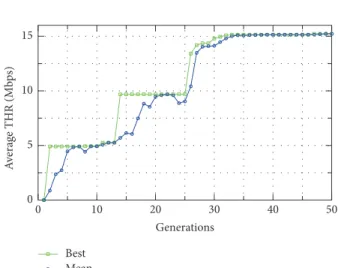
More specifically, Figure 16 depicts the time evolution of the average throughput of the compensating sectors. That is, it shows the performance in terms of the throughput of the6neighbouring cells, which adjust their antenna tilt in order to compensate for the faulty sector. Figure 17 describes the average throughput of the whole network. From this figure, we observe that the GA_𝜃tiltscheme achieves at the30 -th generation23Mbps of average throughput in the whole network, while, in the neighbouring cells (Figure 16), the achieved throughput is only15Mbps, which is reasonable, due to the challenging service conditions in this area.

Finally, the GA_𝜃tilt scheme is compared in Figure 18 with the self-organised Reinforcement Learning- (RL-) based approach for COC proposed in [42], where in order to design the self-healing solution (AC_𝜃_tilt), the antenna tilt is adjusted. The considered RL approach is an Actor Critic algorithm, which is already proven to outperform different solutions for

Best Mean 0.9 1 1.1 A verag e P RB p er Mb 10 20 30 40 50 0 Generations

Figure 15: Evolution of the average PRB per Mb.

Best Mean 0 5 10 15 A verag e THR (Mb ps) 10 20 30 40 50 0 Generations

Figure 16: Evolution of the average throughput in the neighbouring cells. Best Mean 10 15 20 25 A verag e THR (Mb ps) 10 20 30 40 50 0 Generations

Figure 17: Evolution of the average throughput in the whole network.

(14)

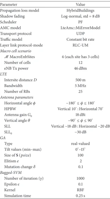
Table 5: Case of study #2: Simulation parameters.

Parameter Value

Propagation loss model HybridBuildings Shadow fading Log-normal, std =8dB

Scheduler PF

AMC model LteAmc::MiErrorModel

Transport protocol UDP

Traffic model Constant bit rate

Layer link protocol-mode RLC-UM Macro cell scenario

MMacroEnbSites 4(each site has 3 cells)

Number of cells 12 eNB Tx power 46dBm LTE Intersite distance𝐷 500m Bandwidth 5MHz Number of RBs 25 Antenna parameters Horizontal angle𝜙 −180∘≤ 𝜙 ≤ 180∘ HPBW Vertical10∘: Horizontal70∘

Antenna gain𝐺₀ 18 dBi

Vertical angle𝜃 −90∘≤ 𝜙 ≤ 90∘

SLL Vertical−18 dB : Horizontal−20 dB

SLL₀ −30 dB

GA

Type real-valued

Tilt values (min–max) 0∘–15∘

Size ofS(𝑝𝑠𝑖𝑧𝑒) 100 Elitism𝑒 2 Mutation change𝛿 0.1 Bagged-SVM Number of iteration (𝛾) 1000 Epsilon𝜖 0.1 Kernel RBF Simulation time 0.25s

COC available in literature in [42]. Therefore, we consider this to be a good benchmark for comparison.

Figure 18 depicts the CDF of the SINR of the network. We assume the user is out of outage when its SINR is above the threshold of−6 dB, as explained in [42]. Therefore, in this figure, we observe that AC_𝜃_tilt is able to recover 95% of UE, while the GA_𝜃tilt is able to recover all the UE. We observe in this figure that, in general, the GA_𝜃tilttends to work effectively, since it maintains the diversity in the values taken by the parameters during the generations and it makes a much deeper estimation of the state of the environment through the regression analysis approach than the AC_𝜃_tilt scheme, which considers only the SINR and CQI feedback from the UE to determine the state of the environment and to estimate the general behaviour of the network.

From these figures, we observe that using the planning tool to adjust the antenna tilt parameter, we are able to

0 0.5 1 CD F −5 0 5 10 15 20 −10 SINR (dB) AC𝜽tilt GA𝜽tilt

Figure 18: CDF of the average SINR values in the faulty sector by two different COC approaches. The GA_𝜃_tiltbased scheme is compared to a RL approach presented in [16].

alleviate the outage caused by the loss of service from a faulty sector.

5. Concluding Remarks

In this paper, we have defined a methodology and built a tool for smart and efficient network planning that exploits and learns from the operational history reflected in the mea-surements gathered anywhere and at any time throughout the network. To build the QoS prediction model based on this historical data, we collect UE measurements according to 3GPP MDT functionality and we apply regression analysis techniques to estimate the Physical Resource Blocks (PRB) per transmitted Mb. This model is then used as objective function in a genetic algorithm (GA_𝜃). By doing this, one can observe that each new iteration increases the efficiency of resource usage in the network while improving the through-put offered to the user.

To demonstrate the flexibility of the proposed smart ML-based planning tool, in this paper, we have decided to apply it to two very different use cases and scenarios: (1) deployment of indoor small cells and (2) compensation of sector faults in a traditional macrocell deployment. For use case #1, results demonstrate the ability of the proposed scheme to deploy small cells in a network in such a way that the average throughput is increased while the PRBs consumed per Mb transmitted decrease, hence improving the spectral efficiency. Regarding use case #2, results demonstrate the ability of the proposed scheme to compensate 100% of outage users in the scenario and to offer them service. We have compared the performance of our approach in the context of the two proposed cases of study to state-of-the-art solutions based on a greedy algorithm for case 1 and reinforcement learning for case 2. Our scheme outperformed state-of-the-art solutions in both cases. We believe that the same technique can be successfully applied to many other planning problems of interest for operators.

(15)

As a future work, we will analyse the planning of scenarios where a huge number of devices have to be provided with service. This is expected to benefit the performance of the estimation, since the data base will be enriched by many measurements, which is the basis of the intelligence of the approach.

Competing Interests

The authors declare that there is no conflict of interests regarding the publication of this paper.

Acknowledgments

The research leading to these results has received funding from the Spanish Ministry of Economy and Competitive-ness FPI Research Programme (BES-2011-047309) under the Grant TEC2010-21100. The work of J. Moysen is also funded by 5GNORM Project (TEC2011-29700-C02-01).

References

[1] 3GPP on track to 5G, http://www.3gpp.org/ news-events/3gpp-news/1787-ontrack 5g.

[2] 5GPPP.The 5G Infrastructure Public Private Partnership, https:// 5g-ppp.eu/.

[3] N. Baldo, L. Giupponi, and J. Mangues-Bafalluy, “Big data empowered self organized networks,” inProceedings of the 20th European Wireless Conference (EW ’14), pp. 181–188, Barcelona, Spain, May 2014.

[4] B. Romanous, N. Bitar, A. Imran, and H. Refai, “Network den-sification: challenges and opportunities in enabling 5G,” in Pro-ceedings of the IEEE 20th International Workshop on Computer Aided Modelling and Design of Communication Links and Net-works (CAMAD ’15), Guildford, United Kingdom, September 2015.

[5] Riverbed OPNET NetOne, https://support.riverbed.com/content/ support/software/steelcentral-npm/net-planner.html.

[6] Cariden MATE Design, Adquired by CISCO, http://www.cisco .com/c/dam/en/us/td/docs/net mgmt/wae/6-1/design/user/ guide/MATE Design User Guide.pdf.

[7] RSoft Design Group. Metrowand, https://optics.synopsys.com/ rsoft/pdfs/RSoftProductCatalog.pdf.

[8] CelPlan. CelTrace TM Wireless Global Solutions, http://www .celplan.com/products/indoor/celtrace.asp.

[9] Net2Plan, “The open-source network planner,” http://www.net-2plan.com/publications.php.

[10] F. Chernogorov and T. Nihtil¨a, “QoS verification for minimiza-tion of drive tests in LTE networks,” inProceedings of the IEEE 75th Vehicular Technology Conference (VTC ’12), pp. 6–9, IEEE, Yokohama, Japan, May 2012.

[11] F. Chernogorov and J. Puttonen, “User satisfaction classification for minimization of drive tests QoS verification,” inProceedings of the IEEE 24th Annual International Symposium on Personal, Indoor, and Mobile Radio Communications (PIMRC ’13), pp. 2165–2169, London, UK, September 2013.

[12] J. Moysen, N. Baldo, L. Giupponi, and J. Mangues-Bafalluy, “Predicting QoS in LTE HetNets based on location-ind-ependent UE measurement,” inProceedings of the 20th IEEE International Workshop on Computer Aided Modelling and

Design of Communication Links and Networks, Guildford, UK, 2015.

[13] J. Moysen, L. Giupponi, and J. Mangues-Bafalluy, “On the potential of ensemble regression techniques for future mobile network planning,” inProceedings of the IEEE Symposium on Computers and Communication (ISCC ’16), pp. 477–483, IEEE, Messina, Italy, June 2016.

[14] D. E. Goldberg,Genetic Algorithms in Search, Optimization, and Machine Learning, Addison-Wesley Longman, Boston, Mass, USA, 1989.

[15] 3GPP, “Radio performance and protocol aspects (system)—RF parameters and BS conformance,” Tech. Rep. TSG RAN WG4 R4-092042, 2009.

[16] J. Moysen and L. Giupponi, “A reinforcement learning based solution for self-healing in LTE networks,” inProceedings of the 80th IEEE Vehicular Technology Conference (VTC ’14-Fall), September 2014.

[17] M. Mitchell,An Introduction to Genetic Algorithms, MIT Press, Cambridge, Mass, USA, 1996.

[18] J. Turkka, F. Chernogorov, K. Brigatti, T. Ristaniemi, and J. Lem-pi¨ainen, “An approach for network outage detection from drive-testing databases,” Journal of Computer Networks and Communications, vol. 2012, Article ID 163184, 13 pages, 2012. [19] F. Chernogorov, S. Chernov, K. Brigatti, and T. Ristaniemi,

Data Mining Approach to Detection of Random Access Sleeping Cell Failures in Cellular Mobile Networks, Computer Science, Networking and Internet Architecture, 2015.

[20] J. Johansson, W. A. Hapsari, S. Kelley, and G. Bodog, “Minimiza-tion of drive tests in 3GPP (Release 11),”IEEE Communications Magazine, 2012.

[21] S. T. Roweis,EM Algorithms for PCA and SPCA, Advances in Neural Information Processing Systems, The MIT Press, 1998. [22] N. S. Altman, “An introduction to kernel and nearest-neighbor

nonparametric regression,”The American Statistician, vol. 46, no. 3, pp. 175–185, 1992.

[23] M. C. Bishop,Pattern Recognition and Machine Learning, Busi-nes Dia, Llc. Springer Science, 2006.

[24] A. J. Smola and B. Sch¨olkopf, “A tutorial on support vector regression,”Statistics and Computing, vol. 14, no. 3, pp. 199–222, 2004.

[25] J. R. Quinlan,Induction of Decision Trees. Machine Learning, Kluwer Academic, 1986.

[26] L. Rokach and O. Maimon,Data Mining with Decision Trees: Theory and Applications, World Scientific, 2008.

[27] D. Opitz and R. Maclin, “Popular ensemble methods: an emp-irical study,”Journal of Artificial Intelligence Research, vol. 11, pp. 169–198, 1999.

[28] L. Rokach, “Ensemble-based classifiers,” inArtificial Intelligence, pp. 1–39, 2010.

[29] T. G. Dietterich, “An experimental comparison of three meth-ods for constructing ensembles of decision trees: bagging, boosting, and randomization,”Machine Learning, vol. 40, no. 2, pp. 139–157, 2000.

[30] T. G. Dietterich, Machine-Learning Research: Four Current Directions, American Association for Artificial Intelligence, 1997.

[31] X. Li, L. Wang, and E. Sung, “AdaBoost with SVM-based com-ponent classifiers,”Engineering Applications of Artificial Intelli-gence, vol. 21, no. 5, pp. 785–795, 2008.

(16)

[32] E. Mayhua-Lopez, V. Gomez-Verdejo, and A. R. Figueiras-Vidal,Boosting Ensembles with Subsampled LPSVM Learners,

Universidad Carlos III de Madrid (UC3M), 2013.

[33] E. Garc´ıa and F. Lozano, “Boosting Support Vector Machines,” inProceedings of the 5th International Conference on Machine Learning and Data Mining in Pattern Recognition, pp. 153–167, Leipzig, Germany, July 2007.

[34] O. Onireti, A. Zoha, J. Moysen et al., “A cell outage management framework for dense heterogeneous networks,”IEEE Transac-tions on Vehicular Technology, vol. 65, no. 4, pp. 2097–2113, 2016. [35] E. J. Khatib, R. Barco, P. Munoz, I. D. La Bandera, and I. Ser-rano, “Self-healing in mobile networks with big data,”IEEE Communications Magazine, vol. 54, no. 1, pp. 114–120, 2016. [36] A. G´omez-Andrades, P. Mu˜noz, I. Serrano, and R. Barco,

“Auto-matic root cause analysis for LTE networks based on unsuper-vised techniques,”IEEE Transactions on Vehicular Technology, vol. 65, no. 4, pp. 2369–2386, 2016.

[37] 3GPP, “Technical specification group radio access network; Evolved universal terrestrial radio access (E-UTRA); Further advancements for E-UTRA physical layer aspects,” Tech. Rep. TR 36.814, 2010.

[38] P. Romanski and L. Kotthoff, “Package FSelector,” https://cran.r-project.org/web/packages/FSelector/FSelector.pdf.

[39] M. Hazewinkel, “Preface,”Discrete Mathematics, vol. 227-228, pp. 1–4, 2001.

[40] J. Moysen, L. Giupponi, and J. Mangues-Bafalluy, “A machine learning enabled network planning tool,” inProceedings of the 27th IEEE Personal Indoor and Mobile Radio Communications (PIMRC ’16), Valencia, Spain, 2016.

[41] F. Gunnarsson, M. N. Johansson, A. Furuskar et al., “Downtil-ted base station antennas—a simulation model proposal and impact on HSPA and LTE performance,” inProceedings of the 68th IEEE Vehicular Technology Conference (VTC Fall ’08), pp. 1–5, Calgary, Canada, September 2008.

[42] J. Moysen and L. Giupponi, “A reinforcement learning based solution for self-healing in LTE networks,” inProceedings of the 80th IEEE Vehicular Technology Conference (VTC Fall ’14), pp. 1–6, IEEE, Vancouver, Canada, September 2014.

(17)