Kent Academic Repository
Full text document (pdf)
Copyright & reuse
Content in the Kent Academic Repository is made available for research purposes. Unless otherwise stated all content is protected by copyright and in the absence of an open licence (eg Creative Commons), permissions for further reuse of content should be sought from the publisher, author or other copyright holder.
Versions of research
The version in the Kent Academic Repository may differ from the final published version.
Users are advised to check http://kar.kent.ac.uk for the status of the paper. Users should always cite the published version of record.
Enquiries
For any further enquiries regarding the licence status of this document, please contact: [email protected]
If you believe this document infringes copyright then please contact the KAR admin team with the take-down information provided at http://kar.kent.ac.uk/contact.html
Citation for published version
Freitas, Alex A. (2019) Automated machine learning for studying the trade-off between predictive
accuracy and interpretability. In: Proceedings of CD-MAKE 2019, Lecture Notes in Computer
Science 11713. . pp. 48-66. Springer ISBN 978-3-030-29725-1. E-ISBN 978-3-030-29726-8.
DOI
https://doi.org/10.1007/978-3-030-29726-8_4
Link to record in KAR
https://kar.kent.ac.uk/77014/
Document Version
Automated Machine Learning for Studying the Trade-off
Between Predictive Accuracy and Interpretability
Alex A. Freitas [0000-0001-9825-4700]
School of Computing, University of Kent, Canterbury, CT2 7NF, UK
Abstract. Automated Machine Learning (Auto-ML) methods search for the best classification algorithm and its best hyper-parameter settings for each input da-taset. Auto-ML methods normally maximize only predictive accuracy, ignoring the classification model’s interpretability – an important criterion in many appli-cations. Hence, we propose a novel approach, based on Auto-ML, to investigate the trade-off between the predictive accuracy and the interpretability of classifi-cation-model representations. The experiments used the Auto-WEKA tool to in-vestigate this trade-off. We distinguish between white box (interpretable) model representations and two other types of model representations: black box (non-interpretable) and grey box (partly (non-interpretable). We consider as white box the models based on the following 6 interpretable knowledge representations: deci-sion trees, If-Then classification rules, decideci-sion tables, Bayesian network classi-fiers, nearest neighbours and logistic regression. The experiments used 16 da-tasets and two runtime limits per Auto-WEKA run: 5 hours and 20 hours. Overall, the best white box model was more accurate than the best non-white box model in 4 of the 16 datasets in the 5-hour runs, and in 7 of the 16 datasets in the 20-hour runs. However, the predictive accuracy differences between the best white box and best non-white box models were often very small. If we accept a predic-tive accuracy loss of 1% in order to benefit from the interpretability of a white box model representation, we would prefer the best white box model in 8 of the 16 datasets in the 5-hour runs, and in 10 of the 16 datasets in the 20-hour runs.
Keywords: Automated machine learning (Auto-ML), classification algorithms, interpretable models.
1
Introduction
This work focuses on the classification task of machine learning, where each instance (example, or data point) consists of a set of predictive features and a class label. A classification algorithm learns a predictive model from a set of training data, where the algorithm has access to the values of both the features and the class labels of the in-stances, and then the learned model can be used to predict the class labels of instances in a separate set of testing data, which was not used during training.
Recently, classification algorithms have been used by an increasingly larger and more diverse set of users, including users with relatively little or no expertise in ma-chine learning. In addition, a large amount of mama-chine learning research has produced many different types of algorithms [5], [19] with increasingly greater complexity. Also, in general these algorithms have several hyper-parameters whose settings need to be carefully tuned to maximize predictive accuracy, for each input dataset.
As a result, recently there has been an increasing research interest in the area of Automated Machine Learning (Auto-ML). In the context of the classification task, Auto-ML methods usually try to solve the problem of finding the best classification algorithm and its best configuration (hyper-parameter settings) for any given dataset provided as input by the user. This is sometimes referred to as the CASH problem – Combined Algorithm Selection and Hyper-parameter optimization [16], [18].
There has also been a growing interest in learning interpretable classification mod-els, motivated by several factors like the need to improve users’ trust on the models’ recommendations, legal requirements for explaining the model’s recommendations in some domains, and the opportunity to provide users with new insight about the data and the underlying application domain [7]. Furtheremore, several studies have dis-cussed how to evaluate the interpretability of classification models – e.g., [7], [8].
Despite this increasing interest in the interpretability of classification models, the classification literature is still overwhelmingly dominated by the use of predictive ac-curacy as the main (and very often the only) evaluation criterion. As a result, the liter-ature is currently dominated by black box classification models, produced by algo-rithms that were designed to maximize predictive accuracy only, without taking into account model interpretability.
This focus on predictive accuracy as the only criterion to evaluate a classification model is particularly strong in the area of Auto-ML, where the interpretability of clas-sification models is normally ignored.
Hence, we propose a novel approach, based on Auto-ML, to investigate the trade-off between the predictive accuracy and the interpretability of classification-model resentations. Note that the focus of this investigation is on the type of knowledge rep-resentation used by the learned classification models, rather than the contents of the models themselves. Broadly speaking, we consider as interpretable the following 6 types of model representation: decision trees, If-Then classification rules, decision ta-bles, Bayesian network classifiers, nearest neighbours and logistic regression represen-tations. Hence, in this work we distinguish mainly between learned models using these representations and learned models using other (non-interpretable or only partly inter-pretable) representations – as discussed in more details in Section 2.2.
Although using an interpretable knowledge representation is not a sufficient condi-tion for a model to be really interpretable by a user, arguably an interpretable represen-tation tends to be a necessary or at least highly desirable condition for obtaining model interpretability. In addition, the full notion of model interpretability involves very sub-jective, user-dependent issues, which are out of the scope of this work.
Hence, in this work we perform a number of experiments with Auto-WEKA, whose search space includes many classification algorithms for learning models with both in-terpretable and non-inin-terpretable representations, and then analyze in detail the results
to investigate to what extent (if any) the best interpretable-representation models pro-duced by Auto-WEKA are sacrificing predictive accuracy by comparison with the best non-interpretable-representation models produced by Auto-WEKA. This is an interest-ing approach to analyze the trade-off between accuracy and interpretability because Auto-WEKA automatically selects the best algorithm and its best hyper-parameter set-tings in a way customized to each input dataset. Hence, the discussion on the trade-off between accuracy and interpretability is raised to a new, more challenging level than usual, where the question is how much accuracy (if any) an interpretable-representation model is sacrificing, not just by comparison with a strong algorithm, but rather by com-parison with the strongest (most accurate) algorithm found by Auto-WEKA for each particular dataset at hand.
Note that, although there are several studies evaluating the performance of Auto-ML methods [10], [6], [14], in general these studies focus only on the predictive accuracy of the selected algorithms, ignoring the issue of the interpretability of their learned models. To the best of our knowledge, this current work is the first one to investigate the trade-off between the predictive accuracy and interpretability of classification mod-els which were optimized to each input dataset by an Auto-ML method.
More precisely, this paper presents the following contributions. First, we investigate the influence of two different runtime limits (as ‘computational budgets’) given to WEKA on the predictive accuracy of the best algorithms selected by Auto-WEKA for each of the 16 datasets used in our experiments. Second, we investigate the frequencies with which different classification algorithms (using different knowledge representations for their learned models) are selected by Auto-WEKA for each dataset, across several runs with different random seeds used to initialize the Auto-WEKA’s search. Third, as the main contribution of this work, we analyze the trade-off between the predictive accuracy and the interpretability of the model representations selected by Auto-WEKA for each dataset.
The remainder of this paper is organized as follows. Section 2 reviews background on Auto-ML and interpretable classification models. Section 3 describes the proposed experimental methodology. Section 4 reports the computational results of the experi-ments with 16 datasets. Section 5 summarizes the results, and Section 6 presents the conclusions and some future research directions.
2
Background
2.1 Background on Automated Machine Learning (Auto-ML)
With the increasing interest in the area of Auto-ML, several types of Auto-ML methods have been proposed in the literature [18], using a variety of search methods to perform a search in the space of candidate machine learning algorithms and their hyper-param-eter settings. However, most Auto-ML methods use, as the search method, some vari-ation of Bayesian Optimizvari-ation (BO) [16], [6] or Evolutionary Algorithms (EAs) [3], [15]. Both BO and EAs are suitable for Auto-ML because they are derivative-free global search methods. That is, they do not require knowledge of the derivative of the
objective function, which is suitable for the discreate search space of candidate solu-tions (involving choices of algorithms), and they perform a global search in the space of candidate solutions, coping with the trade-off between exploitation and exploration in a way that reduces the chances of getting trapped into local optima in the search space. There are also Auto-ML methods based on other types of search methods, like hierarchical planning [14].
Two popular ML tools, representing seminal work in this area, are Auto-WEKA [16] and Auto-sklearn [6], which search in the space of classification algo-rithms offered by the popular WEKA and scikit-learn machine learning libraries, re-spectively – both using BO as the search method. In this work we focus on the Auto-WEKA tool, mainly due to the wide range of classification algorithms considered by this tool – particularly because it includes classification algorithms learning 6 types of interpretable model representations, as discussed in Section 2.2. This is in contrast with e.g. Auto-sklearn, which has a considerably smaller diversity of algorithms learning such interpretable model representations.
The search space considered by Auto-WEKA also includes feature selection meth-ods and their hyper-parameter settings. That is, for each input dataset, the output of Auto-WEKA will be at least a recommended classification algorithm and its hyper-parameter settings, and that output may or may not include also a feature selection al-gorithm and its hyper-parameter settings, applied in a data pre-processing step. In this work, however, we focus only on the classification algorithms selected by Auto-WEKA, since we focus on analyzing the trade-off between the predictive accuracy and interpretability of the models learned by the classification algorithms.
2.2 Background on Interpretable Classification Models
Classification algorithms can be categorized into groups based on the type of knowledge representation used by the classification models that they produce. We em-phasize that this grouping is based on the knowledge representation used by the classi-fication model, i.e., the output of a classification algorithm. This distinction is important because the same type of model can be learned by very different types of algorithms – e.g., decision trees can be learned by a conventional greedy search method or by a more global search method like evolutionary algorithms [1].
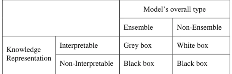
In this work we categorize classification models into 4 broad groups, based on two criteria: (a) whether or not the model is an ensemble (i.e. combining the predictions of a set of base classifiers), and (b) the model’s type of knowledge representation – which can be broadly considered interpretable or non-interpretable. These two criteria are combined into the 2 × 2 matrix shown in Figure 1.
The bottom-right quadrant of the matrix in Figure 1 (non-ensemble, non-interpreta-ble knowledge representation) contains models categorized as black boxes. That is, us-ers cannot normally undus-erstand such black box models in their original form. Examples include, in general, artificial neural networks and support vector machines (SVMs). Note that it is possible to extract interpretable knowledge from a black box model [9], e.g. by extracting a set of rules from neural networks or from SVMs, but in this case of course it is the set of rules which would be interpreted, not the original black box model.
Model’s overall type Ensemble Non-Ensemble
Knowledge Representation
Interpretable Grey box White box
Non-Interpretable Black box Black box
Fig. 1. Categorization of classification models into ‘white box’, ‘black box’ and ‘grey box’ mod-els, based on whether or not the model is an ensemble (combining the outputs of multiple base classifiers) and whether or not the model’s knowledge representation is interpretable.
The bottom-left quadrant of the matrix in Figure 1 (ensemble, non-interpretable knowledge representation) contains models which are also categorized as black boxes. They are in general even harder to interpret than a non-ensemble black box model, due to the typically large number of non-interpretable models in the ensemble.
The top-right quadrant of the matrix in Figure 1 (non-ensemble, interpretable knowledge representation) contains models categorized as white boxes (sometimes called glass boxes [12]). Such models are, at least in principle, directly interpretable by users. In practice, their degree of interpretability varies depending on several factors, including e.g. the user’s understanding about the meaning of the features (attributes) occurring in the model and the user’s understanding about the model’s knowledge rep-resentation. In this work, we consider the following 6 types of knowledge representa-tion as ‘white box’ models: decision trees, If-Then classificarepresenta-tion rules, decision tables, Bayesian network classifiers, nearest neighbours and logistic regression models. The interpretability of the former 5 types of model representations was discussed in detail in [7], whilst logistic regression is also usually recognized as an interpretable type of model in the literature.
Finally, the top-left quadrant of the matrix in Figure 1 (ensemble, interpretable knowledge representation) contains models categorized as ‘grey boxes’. This term is used here to refer to some kinds of ensemble models that are partly interpretable, alt-hough substantially less interpretable than white box models. Broadly speaking, we will refer to an ensemble as a grey box if its base classifiers are white box models, since in principle some approaches for interpreting such white box models can be applied to the ensemble’s members and the results can then be combined to get some interpretability for the ensemble as a whole.
An example of how an ensemble can be partly interpreted involves random forests. In general random forest models are not directly interpretable by users, since they con-tain too many decision trees as base classifiers, and each tree by itself is also hardly interpretable – each tree tends to be large and to have its contents heavily influenced by random samplings of instances and features. Hence, a random forest model is not a white box model. However, random forest models can be partly interpreted by
compu-ting a measure of the importance of each feature across all trees in the forest, and rank-ing the features in decreasrank-ing order of importance. Several such feature importance measures have been proposed in the literature [17], [4]. By using feature importance measures, a random forest model can be considered a grey box model.
3
Experimental Methodology
3.1 Datasets Used in the Experiments
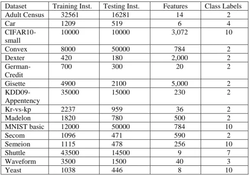
We report the results of experiments using 16 datasets, whose main characteristics are mentioned in Table 1. More precisely, this table shows, for each dataset, its number of training and testing instances, as well as its number of predictive features and class labels. The training and testing sets used here are in general the same as used in the first Auto-WEKA paper [16], and they were in general downloaded from: https://www.cs.ubc.ca/labs/beta/Projects/autoweka/datasets/. The exception is the Adult Census dataset, whose training and testing sets were downloaded from the well-known UCI dataset repository: http://mlr.cs.umass.edu/ml/datasets.html.
Table 1. Main characteristics of the datasets used in the experiments
Dataset Training Inst. Testing Inst. Features Class Labels
Adult Census 32561 16281 14 2 Car 1209 519 6 4 CIFAR10-small 10000 10000 3,072 10 Convex 8000 50000 784 2 Dexter 420 180 2,000 2 German-Credit 700 300 20 2 Gisette 4900 2100 5,000 2 KDD09-Appentency 35000 15000 230 2 Kr-vs-kp 2237 959 36 2 Madelon 1820 780 500 2 MNIST basic 12000 50000 784 10 Secom 1096 471 590 2 Semeion 1115 478 256 10 Shuttle 43500 14500 9 7 Waveform 3500 1500 40 3 Yeast 1038 446 8 10
3.2 Auto-WEKA’s Parameters and Experimental Set Up
The output of Auto-WEKA depends on several user-specified parameters. We specified the values of three of such parameters, as discussed next, and kept the other parameters at their default values.
First, the output of Auto-WEKA naturally depends on the runtime limit (‘computa-tional budget’) specified by the user, i.e. how much time the system is allowed to spend in the search for the best classification/feature selection algorithm and its/their best hy-per-parameter settings for the input dataset. We report results for Auto-WEKA running with 5 hours and 20 hours of runtime limit.
Second, like Auto-ML systems in general, Auto-WEKA is non-deterministic, i.e., its output (selected algorithm and hyper-parameter settings) depends on the random seed number used to initialize the search. We report results of Auto-WEKA with 5 different random seed numbers, for each of the two time limits, for each dataset.
Third, Auto-WEKA’s evaluation function (used to guide the search) was modified from the default ‘error rate’ to the Area Under the ROC curve (AUROC) [13]. The rationale for this modification was that the error rate does not cope well with very im-balanced class distributions, which is the case for several datasets used in the experi-ments. In addition, the AUROC is one of the most used measures of predictive accuracy in practice. The AUROC measure takes values in the range [0..1], with the value 0.5 indicating a predictive accuracy equivalent to that of a random classifier, and 1 indicat-ing the maximal predictive accuracy.
Auto-WEKA was run 10 times (5 seeds × 2 runtime limits) for each dataset. The total time taken by the experiments for each dataset was 125 hours: 25 hours for the 5 runs taking 5 hours each, and 100 hours for the 5 runs taking 20 hours each. So, the total time taken by the experiments for all 16 datasets was 2,000 hours. All experiments were run on a desktop computer with an Intel® Core(TM) i7-7700 CPU with 3.6GHz and 16.0GB of RAM memory.
3.3 The Type of Auto-WEKA’s Output Analyzed in This Work
Recall that the output of Auto-WEKA consists of the best classification algorithm (with its best hyper-parameter settings) selected for the input dataset, and possibly also the best feature selection algorithm (with its best hyper-parameter settings) to be applied in a data pre-processing step. In this work we analyze only on the types of classification algorithms selected by Auto-WEKA, i.e., the analysis of the feature selection algo-rithms output by Auto-WEKA is out of the scope of this work. In addition, we focus on analyzing the output algorithms by themselves, i.e., an analysis of the selected hyper-parameter settings for each algorithm selected by Auto-WEKA is also out of the scope of this work.
Recall that the classification algorithms output by Auto-WEKA have been catego-rized into the three broad groups of white box, black box and grey box models, based on whether or not their learned model is an ensemble and on the broad interpretability of their model’s knowledge representation, as discussed in Section 2.2.
A brief overview of the classification algorithms selected by Auto-WEKA in our experiments (reported in the next Section) is given next, first for ensembles and then for non-ensemble algorithms.
Ensemble Algorithms:
AdaBoost-M1: It learns an ensemble of base classifiers by iteratively re-weighting instances – increasing the weights of instances misclassified in previous iterations.
Bagging (Bag): It learns an ensemble of base classifiers, each of them is learned from randomly sampling instances.
Random Committee (RandCom): It learns an ensemble of randomized base classi-fiers; each is learned from the same data, but using a different random seed number.
Random Forest (RF): It learns a forest (set) of decision trees, each of them is learned by randomly sampling instances and features.
Random SubSpace (RandSS): It learns an ensemble of randomized base classifiers; each is learned by randomly sampling features (creating different feature sub-spaces).
Vote: An ensemble combining the outputs of different types of base classifiers.
Non-Ensemble Algorithms:
BayesNet: It learns a Bayesian network classifier, it can cope with dependences among features (unlike Naïve Bayes).
Decision Table (DecTable): It learns a decision table model, finding a good set of features to be used in the table.
Decision Stump (DecStump): It learns a decision stump, which is a decision tree with just one internal (non-leaf) node.
IBk: A k-nearest neighbour (instance-based learning) classifier.
JRip: It implements the RIPPER algorithm for learning a list of IF-THEN rules.
KStar (K*): A specific type of k-nearest neighbour (instance-based learning) clas-sifier that uses an entropy-based distance function.
Logistic (Log): It learns a multinomial logistic regression model with a ridge esti-mator.
LMT: It learns a Logistic Model Tree, i.e., a decision tree with logistic regression models at the leaf nodes.
LWL: Locally Weighted Learning – It uses an instance-based learning algorithm to assign instance weights, which are then used by a suitable classifier.
MLP: It learns a Multi-Layer Perceptron neural network using backpropagation.
Naïve Bayes (NB): The simplest type of Bayesian network classifier; it assumes that features are independent from each other given the class variable.
PART: Rule induction algorithm that iteratively learns a list of IF-THEN rules, by iteratively converting a learned partial decision tree into a rule.
RepTree: A decision tree learning algorithm designed to be faster than other algo-rithms of this type – it sorts numeric attributes just once.
SimpleLogistic (SimpLog): It learns linear logistic regression models.
SMO: The Sequential Minimal Optimization algorithm for learning an SVM (Sup-port Vector Machine) model.
4
Computational Results
4.1 Analysis of the Influence of the Runtime Limit on Auto-WEKA’s
Predictive Accuracy
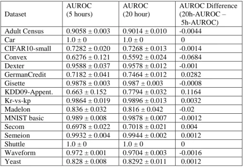
Table 2 shows the mean and standard deviation (over 5 runs varying the random seed) of the Area Under the ROC curve (AUROC) values obtained by the algorithms selected by Auto-WEKA, measured on the test sets, for the experiments with 5 hours and 20 hours of runtime limit. The last column of this table shows the difference between the mean AUROC with 20 hours and the mean AUROC with 5 hours. Hence, a positive (negative) value in that column indicates that increasing the runtime limit from 5 to 20 hours had a positive (negative) effect on the AUROC. The AUROC difference in the last column tends to be larger for datasets with smaller AUROC values, which of course offer more opportunities for larger differences to arise.
In 12 of the 16 datasets included in Table 2, the difference of AUROC between the two runtime limits was very small, smaller than 1%. In the other 4 datasets, however, the runtime limit had a substantial effect: the longer run (20 hours) led to a larger AUROC in two datasets (an increase of 11.6% for KDD09-Appentency and 2.8% for GermanCredit) but to a smaller AUROC in two other datasets (a decrease of 6.8% for Convex and 2% for Madelon). The AUROC values’ standard deviations are in general small, except for the 5-hour runs in two datasets (Convex and KDD09-Appentency).
Table 2. Mean and (after the symbol ±) standard deviation of the AUROC obtained by Auto-WEKA on the test set over 5 runs varying the random seed, with the runtime limit set to 5 hours and 20 hours, and the difference between the two AUROC values.
Dataset AUROC (5 hours) AUROC (20 hour) AUROC Difference (20h-AUROC – 5h-AUROC) Adult Census 0.9058 ± 0.003 0.9014 ± 0.010 -0.0044 Car 1.0 ± 0 1.0 ± 0 0 CIFAR10-small 0.7282 ± 0.020 0.7268 ± 0.013 -0.0014 Convex 0.6276 ± 0.121 0.5592 ± 0.024 -0.0684 Dexter 0.9588 ± 0.037 0.9578 ± 0.012 -0.001 GermanCredit 0.7182 ± 0.041 0.7464 ± 0.012 0.0282 Gisette 0.9878 ± 0.003 0.987 ± 0.003 -0.0008 KDD09-Appent. 0.663 ± 0.152 0.7794 ± 0.032 0.1164 Kr-vs-kp 0.9864 ± 0.019 0.9896 ± 0.013 0.0032 Madelon 0.836 ± 0.032 0.816 ± 0.042 -0.02 MNIST basic 0.989 ± 0.008 0.9878 ± 0.007 -0.0012 Secom 0.6978 ± 0.022 0.7018 ± 0.021 0.004 Semeion 0.9932 ± 0.004 0.9944 ± 0.002 0.0012 Shuttle 1.0 ± 0 1.0 ± 0 0 Waveform 0.972 ± 0.001 0.9704 ± 0.003 -0.0016 Yeast 0.828 ± 0.008 0.8292 ± 0.011 0.0012
We used the non-parametric Wilcoxon signed-rank test of statistical significance to compare the results for 5-hour and 20-hour runs shown in Table 2. Using a two-tailed test and significance level α = 0.05 as usual, we obtained p = 0.94, so the difference of AUROC values among the 5-hour and 20-hour runs is clearly not significant.
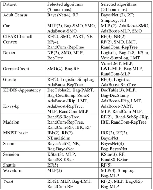
Table 3. Distribution of classification algorithms selected by Auto-WEKA for each dataset across 5 runs, for the runtime limits of 5 hours and 20 hours. The number in brackets after an algorithm’s name represents the selection frequency for that algorithm, out of the 5 runs. The absence of numbers in brackets means the algorithm was selected only once.
Dataset Selected algorithms (5-hour runs)
Selected algorithms (20-hour runs) Adult Census BayesNet(4), RF BayesNet (2), RF;
SimpLog; NB Car MLP(2), Bag-SMO, SMO,
AdaBoost-SMO
MLP (2), AdaBoost-SMO, AdaBoost-MLP, SMO CIFAR10-small RF(2), SMO, PART, NB RF(3), NB(2)
Convex RF(4), RandCom.-RepTree RF(2), SMO, LMT, RandCom.-RepTree Dexter NB(2), SMO, MLP, RepTree
Logistic, Bag-J48, KStar, Vote-SimpLog, LMT
GermanCredit SMO(4), Bag-RF
Vote-LMT, MLP, LWL-MLP, Bag-MLP, RandCom-MLP Gisette RF(2), Logistic, SimpLog,
AdaBoost-RepTree
RF(3), Logistic, AdaBoost-RepTree KDD09-Appentency DecTable(2), Bag-PART,
Bag-DecStump, ZeroR DecTable(3), MLP, Bag-DecStump Kr-vs-kp AdaBoost-JRip, LMT, AdaBoost-RepTree, MLP, RandCom-MLP AdaBoost-JRip, LMT, AdaBoost-PART, MLP, RandCom-MLP, Madelon RandSS-RepTree, RandCom-RepTree, RandCom-RF, IBK, RF RF(2), Rand-SubSp-JRip, IBK, RandCom-RepTree
MNIST basic IBk(2), RF(2), NBmultidim IBK(2), RF(2), BayesNet Secom BayesNet(3), NB, Bag-BayesNet BayesNet(4), Bag-BayesNet Semeion KStar(3), MLP, RandSS-KStar KStar(3), RF, RandSS-KStar Shuttle RF(5) RF(5) Waveform MLP(5) MLP(3), SimpLog, Bag-MLP Yeast RF(2), MLP, Bag-LMT, RandCom-RF RF(2), MLP, Bag-JRip Bag-MLP
We investigated in more detail the results for the KDD09-Appetency dataset, with the largest difference of AUROC between the two runtimes. The large increase in the AUROC value associated with the longer runs of 20 hours is due mainly to the fact that, in the experiments with 5-hour runs, two of the 5 runs achieved a very low AUROC of 0.5 (equivalent to random predictions). In both these runs, the classifier selected by Auto-WEKA was a trivial classifier that simply predicted the most frequent class label to all instances, ignoring the features.
4.2 Analysis of the Distribution of the Classification Algorithms Selected by Auto-WEKA for Each Dataset, Varying Runtime Limit and Random Seed
Table 3 shows the distribution of classification algorithms selected by Auto-WEKA for each dataset, separately for the experiments with runtime limits of 5 hours and 20 hours. Recall that, for each runtime limit, Auto-WEKA was run 5 times for each dataset, var-ying the random seed across runs. For information about the algorithms’ acronyms used in this table, the reader is referred to Section 3.3.
Table 3 shows that there is a wide variety of classification algorithms selected by Auto-WEKA across all datasets. This reinforces the motivation to use an Auto-ML sys-tem to try find the best algorithm for each dataset, supporting the results in [16].
There is also substantial variation among the algorithms selected for each dataset, confirming that the output of Auto-WEKA is sensitive to the random seed number used to initialize its search. However, for some datasets the selection of the best algorithm was reasonably stable across the runs varying the random seed. More precisely, there were 4 algorithms that were selected in the majority (i.e. at least 3) of the 5 runs for each of the two runtime limits (5 hours and 20 hours) for some dataset, as follows. First, Random Forest (RF) was chosen in all 10 runs (5 runs × 2 runtime limits) for the Shuttle dataset. Second, MLP was selected in 8 runs for the Waveform dataset: 5 times with the runtime limit of 5 hours and 3 times with the limit of 20 hours. Third, BayesNet was selected in 7 runs for the Secom dataset: 3 times with the runtime limit of 5 hours, and 4 times with the runtime limit of 20 hours. Fourth, KStar was selected in 6 runs for the Semeion dataset: 3 times for each of the two runtime limits. In addition, when the runtime limit was 5 hours, RF was selected 4 times for the Convex dataset; and when the runtime limit was 20 hours, RF was selected 3 times for the Gisette dataset and 3 times for the CIFAR10-small dataset.
One can also observe in Table 3 that, for the large majority of the datasets, the set of selected algorithms is broadly similar in the two scenarios of 5-hour and 20-hour runs. More precisely, for 13 of the 16 datasets, the intersection between the sets of algorithms selected by Auto-WEKA in the two scenarios has at least 3 (out of 5) algorithms. In one dataset (Shuttle) all 5 selected algorithms were the same (RF) in the two scenarios. However, in two datasets (Dexter and GermanCredit) there was no intersection between the sets of algorithms selected in the two scenarios. As mentioned earlier, for the Ger-manCredit dataset the longer runs led to a somewhat higher AUROC, but for the Dexter dataset the change of selected algorithms between 5-hour and 20-hour runs did not have any substantial effect on the AUROC.
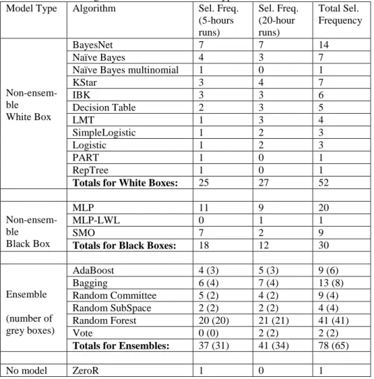
Table 4 shows the selection frequency of each algorithm for all datasets as a whole. In Table 4 the algorithms are divided into the three previously discussed broad groups of algorithms that learn: (a) white box models, (b) black box models, and (c) ensembles, some of which can be considered as ‘grey box’ models if they use white box models as their base classifiers, as discussed in Section 2.2.
Table 4. Selection frequency for each type of model (black box, white box or ensemble model) selected by Auto-WEKA for all datasets as a whole, for each runtime limit (5 hours or 20 hours), and total frequency. In the rows for ensembles, the numbers in brackets are the numbers of ensemble models that can be categorized as ‘grey boxes’, in the sense of consisting of base classifiers that are a type of white box model.
Model Type Algorithm Sel. Freq. (5-hours runs) Sel. Freq. (20-hour runs) Total Sel. Frequency Non-ensem-ble White Box BayesNet 7 7 14 Naïve Bayes 4 3 7
Naïve Bayes multinomial 1 0 1
KStar 3 4 7 IBK 3 3 6 Decision Table 2 3 5 LMT 1 3 4 SimpleLogistic 1 2 3 Logistic 1 2 3 PART 1 0 1 RepTree 1 0 1
Totals for White Boxes: 25 27 52
Non-ensem-ble Black Box MLP 11 9 20 MLP-LWL 0 1 1 SMO 7 2 9
Totals for Black Boxes: 18 12 30
Ensemble (number of grey boxes) AdaBoost 4 (3) 5 (3) 9 (6) Bagging 6 (4) 7 (4) 13 (8) Random Committee 5 (2) 4 (2) 9 (4) Random SubSpace 2 (2) 2 (2) 4 (4) Random Forest 20 (20) 21 (21) 41 (41) Vote 0 (0) 2 (2) 2 (2)
Totals for Ensembles: 37 (31) 41 (34) 78 (65)
No model ZeroR 1 0 1
Let us first discuss in more detail the results for white box and black box models. As a whole, white box models were selected more often than black box models in both the
experiments with 5 hours of runtime limit and the experiments with 20 hours. The dif-ference of selection frequency in favour of white box models is considerably larger for the 20-hour runs (27 white box models vs. 12 black box models) than for the 5-hour runs (25 vs. 18).
The most frequently selected type of white box model was BayesNet, which was selected 14 times in total (adding the selection frequencies for both runtime limits). In addition, Naïve Bayes was the second most frequently selected white box classifier, with a total frequency of 8 (including one selection of its variant Naïve Bayes multino-mial); and since both BayesNet and Naïve Bayes are instantiations of a Bayesian net-work classifier, this broad type of model was selected in total 22 times.
The second most frequently selected broad type of white box model was nearest neighbours, with the KStar and IBk algorithms selected 7 and 6 times, respectively – i.e., 13 times in total.
Other types of white box models had smaller but still substantial selection frequen-cies, as follows. DecisionTable was selected 5 times. LMT (Logistic Model Trees) was selected 4 times. Note that a LMT model is a hybrid decision tree / logistic regression model (it is a decision tree with logistic regression models at the leaf nodes). A stand-alone logistic regression model was selected 6 times (3 times with the Logistic algo-rithm and 3 times with the SimpleLogistic algoalgo-rithm).
Decision trees by themselves (i.e., not counting their use in ensembles) had a sur-prising low selection frequency. Not counting the 4 times a LMT model was selected, a stand-alone decision tree model was selected just once, with the RepTree algorithm – which was designed to be fast (not just to maximize accuracy), i.e., it may sacrifice some accuracy to gain computational efficiency.
The black box models selected by Auto-WEKA were less diverse than the white box models; more precisely, MLP was selected 21 times (one of them using LWL – Local Weighted Learning – to assign weights to instances), whilst SMO (a type of SVM al-gorithm) was selected 9 times.
We now turn to ensembles. As a whole, ensembles were the type of algorithm most frequently selected by Auto-WEKA, for both runtime limits (5 and 20 hours). In total, ensembles were selected in 78 out of the 160 cases (i.e., in about 49% of the cases). The overall success of ensembles is not surprising, due to their advantages stemming from combining diverse base models to achieve a more effective classifier [20].
By far the most selected type of ensemble model was Random Forest, which was selected 41 times in total (i.e., in about 23% of the 180 cases). Bagging, AdaBoost-M1 and Random Committee were also selected quite often by Auto-WEKA, in total 13, 9 and 9 times, respectively. Random SubSpace and Vote were selected only 4 and 2 times, respectively.
Recall that we considered as ‘grey box’ models the ensembles that can be partly interpreted, due to their base classifiers being interpretable (white box) models. Hence, in the rows for ensemble models in Table 4, the numbers in brackets are the numbers of models that can be categorized as ‘grey boxes’.
Note that, since random forests consist of partly random decision tree models, and many feature importance measures for random forests are available in the literature as mentioned earlier, all 41 random forest models mentioned in Table 4 can be considered
grey box models. The other types of ensemble models in Table 4 also have a high pro-portion of grey box models in general. Actually, considering all types of ensemble mod-els in Table 4 for the two runtime limits of 5 hours and 20 hours, 65 out of the 78 ensemble models (i.e., about 83%) can be considered grey box models. It should be emphasized, however, that a grey box model is still considerably less interpretable than a white box model, and it requires substantial post-processing for interpretability. That is, after the ensemble is constructed, typically we still need to run some post-processing procedure (e.g. the aforementioned feature importance measures). By contrast, such post-processing is not usually required in the case of white box models, which can be more directly interpreted. A detailed investigation of to what extent such grey box, partly interpretable models can be really (subjectively) interpreted by users in practice is beyond the scope of this work.
4.3 Analysis of the Trade-off Between the Predictive Accuracy and the Interpretability of the Selected Classification Models
Recall that Auto-WEKA’s search is guided by an evaluation function that is based on estimating only the predictive accuracy of the candidate algorithms, without consider-ing the interpretability of their learned models. Despite this, for any given dataset, it is possible that the best algorithm selected by Auto-WEKA for a given input dataset is an algorithm that learns a white box model, in which case we would get the benefit of a model with an interpretable knowledge representation without sacrificing accuracy.
As mentioned in the Introduction, there is a growing importance of interpretability in the classification task of machine learning, due to the increasingly large number of applications of classification algorithms across many domains. Despite this, the litera-ture is still overwhelmingly dominated by the goal of maximizing predictive accuracy, with relatively little emphasis on learning interpretable models. That is, most research-ers and practitionresearch-ers focus on using only black box or ensemble models, without even trying algorithms that learn at least potentially interpretable models. It is not clear how often this leads to missing the opportunity of learning an interpretable model that is almost as accurate as a black box or ensemble model. Hence, it is important to investi-gate this trade-off between predictive accuracy and interpretability by considering a wide range of algorithms.
Auto-ML systems like Auto-WEKA provide an interesting novel perspective for this investigation, because Auto-WEKA automatically searches for the best algorithm for the input dataset, in a search space that includes both many algorithms learning white box models and many algorithms learning black box or ensemble models.
In this context, the important research question addressed in this section is: to what extent does the best white box model recommended by Auto-WEKA (for the input da-taset) sacrifice predictive accuracy, by comparison with the best non-white box (i.e. black box or ensemble) model recommended by Auto-WEKA?
To investigate this issue, for each dataset, and for each of the two runtime limits (5 hours and 20 hours), Table 5 reports two types of AUROC values, both measured on the test set: (a) the highest AUROC among the non-white box (i.e., black box and
en-semble) models produced by the algorithms selected by Auto-WEKA in its 5 runs var-ying the random seed; and (b) the highest AUROC among the white box models pro-duced by the algorithms selected by Auto-WEKA in its 5 runs. Each cell of Table 5 also indicates, below the AUROC value, the name of the algorithm(s) which obtained that result. If none of the 5 algorithms selected by Auto-WEKA for a given pair of dataset and runtime limit learns the type of model associated with the corresponding table column, the corresponding cell in Table 5 has the keyword ‘none’.
Hence, in order to determine to what extent the selected white box models are sacri-ficing predictive accuracy by comparison with the best non-white box model found by Auto-WEKA, for each dataset and runtime limit, one can compare two pairs of columns in Table 5: the second and third columns (5-hour runs), and the fourth and fifth columns (20-hour runs). The best result for each dataset and each run time limit is shown in boldface font.
For the 5-hour runs, the best white box model achieved a higher AUROC than the best non-white box model in only 4 of the 16 datasets. In those 4 datasets, the gain in predictive accuracy associated with the best white box model (versus the best non-white box model) was: 0.5% for Adult Census, 0.9% for Semeion, 1.8% for Dexter, and 7.3% for KDD09-Appetency. However, no white box model was selected in the 5 Auto-WEKA runs for 6 datasets. Regarding the remaining 6 datasets, it is interesting to note that the loss of predictive accuracy associated with the best white box model (versus the best non-white box model) was very small (less than 0.5%) in 4 of those datasets. More precisely, these AUROC losses were: 0.1% for kr-vs-kp and MNIST Basic, 0.2% for Gisette, 0.4% for CIFAR10-small, 3.6% for Secom, 8% for Madelon.
For the 20-hour runs, the best white box model achieved a higher AUROC than the best non-white box model in 7 of the 16 datasets. In those 7 datasets, the gain in pre-dictive accuracy (AUROC value) associated with the best white box model (versus the best non-white box model) was: 0.4% for Dexter and Semeion, 0.5% for Adult Census, 0.9% for MNIST Basic, 1.0% for KDD09-Appetency, 2.7% for Secom, and 2.9% for CIFAR10small. However, no white box model was selected in the 5 Auto-WEKA runs for 4 datasets. Regarding the remaining 5 datasets, it is interesting to note that the loss of predictive accuracy associated with the best white box model (versus the best non-white box model) was very small (less than 1%) in 3 of those datasets. More precisely, these AUROC losses were: 0.1% for kr-vs-kp, 0.2% for Gisette, 0.7% for Waveform, 2.8% for Convex, and 4.8% for Madelon.
We used the non-parametric Wilcoxon signed-rank test of statistical significance to compare the aforementioned two pairs of results in Table 5, i.e., to compare the results for the best non-white box vs. the results for the best white box model, for each runtime limit (5 hours and 20 hours). For this comparison, the cases where no white box model was selected were assigned an AUROC of 0. Using a two-tailed test and significance level α = 0.05 as usual, we obtained p = 0.0349 and p = 0.2846 for the 5-hour and 20-hour runs, respectively. Hence, the difference of predictive accuracy between the best non-white box models and the best white box models is statistically significant (in fa-vour of non-white box models) for the 5-hour runs, but not statistically significant for the 20-hour runs.
Table 5. AUROC (on the test set) of the best non-white box model (i.e. the best among black box and ensemble models) and the best white box models, separately for 5-hour and 20-hour runs. In each cell, the name of the algorithm(s) producing the corresponding best model is shown below the AUROC value. The best result for each pair of dataset and runtime limit is shown in boldface font.
Dataset 5-hour runs 20-hour runs best non-white box model best white box model best non-white box model best white box model Adult Census 0.903 Rand. Forest 0.908 BayesNet 0.903 Rand. Forest 0.908 BayesNet Car 1.0 SMO,MLP, Bagg.,AdaBo. none 1.0 SMO,MLP, AdaBoost none CIFAR10-small 0.751 SMO 0.747 Naïve Bayes 0.718 Rand. Forest 0.747 Naïve Bayes Convex 0.844
Rand. Forest none
0.584 Rand. Forest 0.556 LMT Dexter 0.973 MLP 0.991 Naive Bayes 0.965 Vote 0.969 LMT German-Credit 0.753 SMO none 0.762 Vote none Gisette 0.991 AdaBoost 0.989 Log.,Sim-pLog. 0.991 AdaBoost 0.989 Logistic KDD09-Appentency 0.723 Bagging 0.796 DecTable 0.786 MLP 0.796 DecTable Kr-vs-kp 1.0 AdaBoost 0.999 LMT 1.0 AdaBoost 0.999 LMT Madelon 0.891 Rand. Com. 0.811 IBk 0.859 Rand. Forest 0.811 IBk MNIST basic 0.996 Rand. Forest 0.995 IBk 0.986 Rand. Forest 0.995 IBk Secom 0.735 Bagging 0.699 Naive Bayes 0.708 Bagging 0.735 BayesNet Semeion 0.987 MLP 0.996 KStar 0.993 Rand. SubSp. 0.997 KStar Shuttle 1.0
Rand. Forest none
1.0
Rand. Forest none
Waveform 0.973 MLP none 0.973 MLP, Bagg. 0.966 SimpleLo-gistic Yeast 0.835
Rand. Comm. none
0.839
Rand. Forest none
5
Summary of Results and Discussion
Regarding the influence of the runtime limit on the predictive accuracy of Auto-WEKA, the difference between the mean AUROC values for the experiments with 5 hours and 20 hours of runtime limit was smaller than 1% in 12 of the 16 datasets; and overall (across all datasets) the difference was not statistically significant.
Regarding the frequencies with which different classification algorithms are selected by Auto-WEKA for each dataset, Auto-WEKA selected a wide variety of classification algorithms across the 16 datasets. This supports the motivation to use an Auto-ML sys-tem to try to find the best algorithm with its best hyper-parameter settings for each dataset.
For most datasets, the difference between the sets of classification algorithms lected by Auto-WEKA with 5-hour runs and 20-hour runs is not large, i.e., several se-lected algorithms tend to be the same for both runtime limits.
In any case, in practice it seems important to run Auto-WEKA several times for the same dataset by varying the random seed across the runs, since for most datasets there was a substantial diversity of selected algorithms across different runs – which was observed with both 5 hours and 20 hours of runtime limit.
Ensembles were selected by Auto-WEKA as the best algorithm in about 49% of the cases (in 78 out of 160 cases). The high prevalence of ensembles was consistently ob-served for both runtime limits (5 hours and 20 hours). In addition, the model type most frequently selected by Auto-WEKA was random forest, an ensemble considered a grey box model (see Section 2.2), which was selected 41 times in total – over both 5-hour and 20-hour runtime limits. Among non-ensembles, white box and black models were selected in 52 (32.5%) and 30 (18.75%) of the 160 cases, respectively.
The most frequently selected type of white box model was Bayesian network classi-fiers – more precisely, 14 selections of BayesNet and 8 selections of standard Naïve Bayes or its multinomial variant. Although a Naïve Bayes model can be easily inter-preted due to its simplifying assumption that features are independent of each other given the class variable, the interpretation of BayesNet becomes more difficult as more and more feature dependencies are included in the network. In the general case of Bayesian network. For instance, Heckerman et al. [11] have pointed out that users can get confused with the interpretation of (in)dependence relationships represented in Bayesian networks, and suggested an alternative knowledge representation of depend-ence networks that seems to have improved interpretability.
We also analyzed the difference of predictive accuracy (AUROC values) between the best white box model and the best non-white box model selected by Auto-WEKA for each dataset.
Overall, the best white box model achieved a higher AUROC than the best non-white box model in only 4 of the 16 datasets in the experiments with 5 hours of runtime limit, and in 7 out of 16 datasets in the experiments with 20 hours of runtime limit. However, the loss of predictive accuracy associated with the best white box model (ver-sus the best non-white box model) was smaller than 0.5% for 4 datasets in the 5-hour experiments, and smaller than 1% for 3 datasets in the 20-hour experiments. The higher
AUROC values associated with the best non-white box models was statistically signif-icant in the 5-hour experiments, but not in the 20-hour experiments.
6
Conclusions and Future Work
We have proposed the use of Automated Machine Learning (Auto-ML) methods as a novel approach to investigate the trade-off between the predictive accuracy and inter-pretability of classification models. The experiments involved 160 runs of Auto-WEKA (a popular Auto-ML tool) – 10 runs for each dataset, varying the runtime limit (com-putational budget) and the random seed across the runs.
In this work classification algorithms were divided into the following groups (as summarized in Figure 1): white box non-ensemble models (potentially fully interpret-able), black box non-ensemble models (not interpretable) and ensembles – some of them considered partly interpretable grey box models; whilst other ensembles are black boxes.
Overall, the algorithm type most selected by Auto-WEKA were ensembles, with the random forest ensemble in particular being the most selected algorithm type. Among non-ensembles, algorithms producing white box models were selected more often than algorithms producing black box, and variations of Naïve Bayes and Bayesian network classification algorithms were the most selected type of algorithm producing white box models.
Finally, we used Auto-WEKA’s automated search for the best algorithm for each dataset as an approach to address the following research question: “to what extent does the best white box model recommended by Auto-WEKA (for the input dataset) sacri-fice predictive accuracy, by comparison with the best non-white box (i.e. black box or ensemble) model recommended by Auto-WEKA?”
The results have shown the loss of predictive accuracy (AUROC value) associated with the best white box model – by comparison with the best non-white box – is often small, in several cases being smaller than 1%.
In application domains where interpretability is very important, an accuracy loss of 1% seems an acceptable price to pay for the benefit of having a white box, interpretable model, instead of a non-interpretable model – see e.g. the discussion in [2], where in-terpretable logistic regression models were preferred by the user over substantially more accurate but non-interpretable neural network models in a medical domain.
If we consider an accuracy loss of 1% as acceptable in order to get the benefits of an interpretable model representation (which is an application domain-dependent decision in practice), the main conclusions are as follows. For the 5-hour experiments, we would prefer the best white box model over the best non-white box one in 8 out of the 16 datasets (with the best white box model being more accurate in 4 datasets). For the 20-hour experiments, we would prefer the best white box model in 10 of the 16 datasets (with the best white box model being more accurate in 7 datasets).
Note, however, that this work considered as white box all models using some inter-pretable knowledge representation, without analyzing the internal details of the models to check if they are really (subjectively) interpretable by users.
As future work, it would be interesting to perform experiments with other Auto-ML tools and more datasets. In addition, although we have to some extent discussed the potential interpretability of ensemble models where the base classifiers are white box models, this is a complex issue that deserves more investigation in future work.
References
1. Barros, R.C., Basgalupp, M.P., de Carvalho, A.C.P.L.F., Freitas, A.A. A Survey of Evolutionary Algorithms for Decision Tree Induction. IEEE Transactions on Sys-tems, Man and Cybernetics – Part C: Applications and Reviews, 42(3), 291-312. May 2012.
2. Caruana, R., Lou, Y., Gehrke, J., Koch, P., Sturm, M., Elhadad, N. Intelligible mod-els for healthcare: predicting pneumonia risk and hospital 30-day readmission. Proc. ACM SIGKDD Int. Conf. on Knowledge Discovery and Data Mining (KDD’15), 1721-1730. ACM, 2015.
3. de Sa, A.G.C., Freitas, A.A., Pappa, G.L. Automated selection and configuration of multi-label classification algorithms with grammar-based genetic programming. In Proc. 15th Int. Conf. on Parallel Problem Solving from Nature (PPSN XV), Part II
– LNCS 11102, 308-320. Springer, 2018.
4. Epifanio, I. Intervention in prediction measure: a new approach to assessing variable importance for random forests. BMC Bioinformatics 18, 230, 2017.
5. Fernandez-Delgado, M., Cernadas, E., Barro, S., Amorin, D. Do we need hundreds of classifiers to solve real world classification problems? Journal of Machine Learn-ing Research 15, 3133-3181, 2014.
6. Feurer, M., Klein, A., Eggensperger, K., Springenberg, J., Blum, M., Hutter, F. Ef-ficient and robust automated machine learning. In: Proc.Advances in Neural
Infor-mation Processing Systems, 2962-2970, 2015.
7. Freitas, A.A. Comprehensible classification models. ACM SIGKDD Explorations, 15(1), 1-10. 2013.
8. Furnkranz, J., Kliegr, T., Paulheim, H. On cognitive preferences and the interpreta-bility of rule-based models. arXiv preprint: arXiv:1803.01316v2 [cs.LG], 10 Mar 2018.
9. Guidotti, R., Monreale, A., Turini, F., Pedreschi, D., Giannotti, F. A survey of meth-ods for explaining black box models. arXiv:1802.01933v1 [cs.CY] 6 Feb. 2018
10. Guyon, I., Chaabane, I., Escalante, H.J., Escalera, S., Jajetic, D., Lloyd, J.R., Macia, N., Ray, B., Romaszko, L., Sebag, M. and Statnikov, A.. A brief review of the ChaLearn AutoML challenge: any-time any-dataset learning without human inter-vention. Proc. ICML 2016 AutoML Workshop, published as JMLR: Workshop and Conference Proceedings 64: 21-30, 2016.
11. Heckerman, D., Chickering, D.M., Meek, C., Rounthwaite, R., and Kadie, C. De-pendency networks for inference, collaborative filtering and data visualization.
Journal of Machine Learning Research 1, 49-75, 2000.
12. Holzinger, A. Interactive machine learning for health informatics: when do we need the human-in-the-loop? Brain Informatics, 3(2), 119-131, 2016.
13. Japkowicz, N. and Shah, M. Evaluating Learning Algorithms: a classification per-spective. Cambridge University Press, 2011.
14. Mohr, F., Wever, M. and Hüllermeier, E., 2018. ML-Plan: Automated machine learning via hierarchical planning. Machine Learning, 107(8-10), 1495-1515.
15. Olson, R.S., Bartley, N., Urbanowicz, R.J., Moore, J.H. Evaluation of a tree-based pipeline tool for automating data science. Proc. Genetic and Evolutionary
Compu-tation Conf. (GECCO-2016), 8 pages, 2016.
16. Thornton, C. et al. Auto-Weka: combined selection and hyperparameter optimiza-tion of classificaoptimiza-tion algorithms. Proc. 19th ACM SIGKDD Int. Conf. on Knowledge Discover & Data Mining, 847–855, ACM, 2013.
17. Verikas, A., Gelzinis, A., Bacauskiene, M. Mining data with random forests: a sur-vey and results of new tests. Pattern Recognition 44, 330-349, 2011.
18. Yao, Q., Wang. M., Escalante, H.J., Guyon, I., Hu, Y.-Q., Li, Y.-F., Tu, W.-W., Yang, Q., Yu, Y. Taking human out of learning applications: a survey on automated machine learning. arXiv preprint arXiv:1810.13306, 31 Oct. 2018.
19. Zhang, C., Liu, C., Zhang, X., Almpanidis, G. An up-to-date comparison of state-of-the-art classification algorithms. Expert Systems with Applications, 82, 128-150, 2017.