Evolving and Ensembling Deep CNN Architectures for Image Classification

(1)

Citation: Fielding, Ben, Lawrence, Tom and Zhang, Li (2019) Evolving and Ensembling Deep

CNN Architectures for Image Classification. In: IJCNN 2019 - 2019 International Joint

Conference on Neural Networks, 14th - 19th July 2019, Budapest, Hungary.

URL:

This version was downloaded from Northumbria Research Link:

http://nrl.northumbria.ac.uk/40456/

Northumbria University has developed Northumbria Research Link (NRL) to enable users to

access the University’s research output. Copyright

©

and moral rights for items on NRL are

retained by the individual author(s) and/or other copyright owners. Single copies of full items

can be reproduced, displayed or performed, and given to third parties in any format or

medium for personal research or study, educational, or not-for-profit purposes without prior

permission or charge, provided the authors, title and full bibliographic details are given, as

well as a hyperlink and/or URL to the original metadata page. The content must not be

changed in any way. Full items must not be sold commercially in any format or medium

without formal permission of the copyright holder. The full policy is available online:

http://nrl.northumbria.ac.uk/policies.html

This document may differ from the final, published version of the research and has been

made available online in accordance with publisher policies. To read and/or cite from the

published version of the research, please visit the publisher’s website (a subscription may be

required.)

(2)

Evolving and Ensembling Deep CNN Architectures

for Image Classification

Ben Fielding

Computer and Information Sciences Northumbria University Newcastle upon Tyne, UK [email protected]

Tom Lawrence

Li Zhang

Abstract—Deep Convolutional Neural Networks (CNNs) have

traditionally been hand-designed owing to the complexity of their construction and the computational requirements of their training. Recently however, there has been an increase in research interest towards automatically designing deep CNNs for specific tasks. Ensembling has been shown to effectively increase the performance of deep CNNs, although usually with a duplication of work and therefore a large increase in computational resources required. In this paper we present a method for automatically designing and ensembling deep CNN models with a central weight repository to avoid work duplication. The models are trained and optimised together using particle swarm optimisation (PSO), with architecture convergence encouraged. At the conclusion of the joint optimisation and training process a base model nomination method is used to determine the best candidates for the ensemble. Two base model nomination methods are proposed, one using the local best particle positions from the PSO process, and one using the contents of the central weight repository. Once the base model pool has been created, the individual models inherit their parameters from the central weight repository and are then finetuned and ensembled in order to create a final system. We evaluate our system on the CIFAR-10 classification dataset and demonstrate improved results over the single global best model suggested by the optimisation process, with a minor increase in resources required by the finetuning process. Our system achieves an error rate of 4.27% on the CIFAR-10 image classification task with only 36 hours of combined optimisation and training on a single NVIDIA GTX 1080Ti GPU.

Index Terms—Deep Learning, Evolutionary Computation,

Image Classification, Convolutional Neural Networks, Particle Swarm Optimisation

I. INTRODUCTION

Convolutional neural networks (CNNs) are a class of neural networks that are used to learn filters (or kernels) from feature maps, often in a sequential or hierarchical manner. The depth of a CNN usually refers to the number of convolutional layers that sequentially process feature maps, where the output of one layer is used as the input to the following layer. CNNs have been heavily used for computer vision tasks since Krizhevsky et al. [1] used a deep CNN to beat the nearest competitor by more than 10% on the Imagenet Large Scale Visual Recogni-tion Challenge (ILSVRC) [2] in 2012. Since then, CNNs have been used as effective feature extractors in a huge number of computer vision areas, such as image description generation [3], intelligent visual agents [4], [5], visual question answering [6], visual dialog [6], and many more. Current methods to

use CNNs as feature extractors often rely on transfer learning using one of a small number of pre-conceived architectures, as designing a new architecture by hand can require in-depth knowledge of complex parameters. Therefore, techniques are required to automatically generate new CNN architectures, specific to the task at hand, allowing more versatility and better task-specific performance than ‘borrowed’ architectures.

Ensembling techniques have been shown to improve deep convolutional neural network (CNN) performance, even when assembled from identical architecture models. GoogleNet [7] used an ensemble of seven identical individuals to reduce the top-5 error rate on the ImageNet ILSVRC 2014 classification

challenge dataset from10.07%to6.67%, a reduction of3.45%

over their single model result. Szegedy et al. [8] showed that combining similar, but not identical, Inception model architectures also produced improved performance over a single model. Using the Imagenet ILSVRC 2012 classification challenge dataset, they showed a reduction in error rate from

17.8% for the best performing single model, down to 16.4%

for an ensemble of four models using two different architecture choices. Performance increases such as these represent an attractive way to improve accuracy scores for a model, as they only require more computational resources, rather than modifications to the model itself. Consequently they can theoretically be performed on any deep CNN, given enough resources. However, this duplication of work represents a linear increase in resource costs, often in exchange for a minor increase in accuracy. Recent works [9], [10] show that ensembles can be constructed effectively without a linear increase in computational work.

In this paper, we demonstrate techniques for constructing ensembles from the outcome of an evolutionary CNN architec-ture search using enhanced particle swarm optimisation (PSO). The search process itself uses a weight sharing technique to avoid duplicating training efforts between the individuals when performing each fitness evaluation, meaning that models with the exact same architecture configuration will share weights and be functionally identical networks. Following the optimisation process, we propose two techniques for nomi-nating candidate base models to be ensembled for the final system. One technique uses the remaining local best particle positions from the PSO process, which are clustered around

(3)

the global best position due to the nature of PSO. The other technique uses the central weight sharing repository that is utilised by the optimisation process to jointly train the models during optimisation. Following base model identification, the individual models are then fine-tuned on a combination dataset in order to reduce overfitting. Once the base models have been fine-tuned, their individual and group ensemble performance on the test set is evaluated and provided alongside similar related works and the results are discussed.

The remainder of the paper is structured as follows: Section II discusses relevant related work in the area, Section III describes our methodology in designing and implementing the system, Section IV discusses our experimental results and findings, and Section V contains concluding remarks and plans for future work given these findings.

II. RELATEDWORK

Bagging [11] and AdaBoost [12] are popular methods for constructing ensembles with data variants. More specifically, numerous models are created by dividing the training data into smaller subsets, each subset is then used to train a model. At test time, a sample is passed through each model and an average is taken to give the final prediction. Khatami et al. [13] showed ensembles gave considerable improvements and cutting-edge results in the domain of medical image retrieval which suffers from strongly imbalanced datasets. The proposed architecture consisted of an ensemble of three hand-crafted convolutional neural networks based on LeNet [14], each trained with different structures and learning schemes aimed at reducing the output of each network to two possible outputs and probabilities, thus greatly reducing the search space to a potential six. Huang et al. [15] showed that once an architecture has been selected, the computational cost of generating multiple models for ensembling can be reduced by converging at multiple local minima and saving the model parameters along its optimization path. Once complete, an average of the discovered models was taken at test time and a performance increase was observed. Hara et al. [16] proposed the idea that regularisation methods such as Dropout can be considered to be ensembling techniques. They showed that model accuracy can be improved by taking an average over a network with learned and unlearned units. Huang et al. [17] proposed the idea of using stochastic depth as an ensembling technique by taking average outputs over networks with missing layers. Singh et al. [18] proposed swapout, an ensembling technique that combines both dropout and stochastic depth approaches.

A common problem to many of these approaches is the extensive domain knowledge required in order to construct the initial base models to be ensembled. Recent works have addressed this requirement through the proposal of evolution-ary search techniques for ensemble construction and CNN architecture generation.

Zhang et al. [19] proved with extensive benchmarking that evolutionary generated ensembles based on the firefly algorithm can outperform state of the art variants by extending

the attractiveness behaviour with the introduction of evading action. Attractiveness considered the global best rather than just neighbours, and the evading action was informed by the global and local worst. These two attributes combined drove the fireflies to converge quickly by efficiently vacating unpromising regions resulting in a more efficient method for finding the best solution. By splitting the fireflies into subswarms, multiple solutions could be found, thereby gener-ating an entire ensemble. EUSBoost [20] used an evolutionary approach which promoted diversity between ensembles using the Q-statistic diversity measure as a form of guided boosting. Bochinski et al. [21] proposed an evolutionary approach to hyper-parameter optimisation and showed that applying such a technique for an ensemble of multiple CNNs gave significant improvements on the MNIST dataset for hand-written digit recognition when compared to handcrafted architectures such as LeNet-5 [14]. Wang et al. [22] used PSO to find an optimal CNN architecture, automating the process of making architectural choices such as filter sizes, stride, layer types, network depth and width. The resulting architecture, however, did not consistently outperform handcrafted architectures. Real et al. [23], [24] recently presented an evolutionary generated architecture which outperformed hand-designed architectures. The method introduced an age property to an evolutionary algorithm which promoted exploration within the search rather than ‘zooming in’ on a good candidate too early. Moyano et al. [25] showed that over a range of 14 datasets tested, an evolutionary approach based on a generational elitist algo-rithm could automatically generate diverse classifiers which performed more statistically accurately and consistently when compared to state of the art approaches. Zhao et al. [26] found that by introducing an objective of sparseness to be minimised, multiple evolutionary algorithms with different ob-jectives could construct multiple models of smaller classifiers which had the ability to generalise well together. Ultimately, an ensemble could be discovered which was multi-objective focused, diverse, and performed competitively. Fielding and Zhang [27] used an enhanced PSO variant to efficiently nav-igate a block-based CNN search space, using weight-sharing techniques to alleviate the enormous time and resource cost of the fitness function evaluation. The method jointly evolved and trained a single effective CNN architecture in around 34 hours using a single consumer GPU.

III. METHODOLOGY

A. Base Model Generation

Following [27], we use the SOBA method for jointly optimising and training block architecture models. SOBA is a technique whereby a population of individuals explore a search space of architecture design decisions whilst cooperatively training their internal parameters. The individuals consist of deep CNNs constructed in a block-wise manner, where each block of an individual architecture represents a portion of a linear convolutional graph. The graphs are portioned according to a scheduled increase in depth (of convolutional filter banks) alongside a decrease in spatial size (of feature

(4)

map). For this implementation, each architecture then consists of five key design decisions, mapping to five distinct blocks in the architecture. The first block, or architecture decision,

takes an image as input (32×32×3 for CIFAR-10) and

consists of 1. . . n convolutional layers, with accompanying

BatchNorm and ReLU activation. The first convolutional layer in the block is used to increase the depth of the subsequent

feature maps from 3 to64, which is then maintained for the

remainder of the block. The subsequent three blocks are also convolutional blocks and follow the same practice, whereby the first convolutional layer in each block increases the number

of feature maps to 2 _where _{takes the values} _[7_,₈_,_9]_{. The}

final block in the architecture controls the number of linear classification layers at the end of the network. Prior to this block, the output of the previous (convolutional) block is flattened and then used as input into an initial dense layer. This first dense layer consists of a simple linear layer of single neurons connecting the flattened convolutional layer to a layer

output of size 4096. The subsequent layers in this block are

then simply linear layers mapping input vectorsR4096to layer

output vectors R4096. The final layer in the architecture is a

linear layer which maps the output of the final block (R4096)

to the number of output classes (R10for CIFAR-10). We then

perform a softmax over the final output vector to calculate the probability of the input image belonging to each individual class.

B. Particle Swarm Optimisation

The optimisation process uses particle swarm optimisation (PSO) to evolve a swarm of individual particles representing different architecture choices, initialised as random positions in the search space. The particle positions are updated using the standard PSO methodology with modifications to the acceleration coefficients as proposed by [27]. First the velocity is updated taking into account the previous best position of the individual being updated, and the previous best position overall. The velocity update can be seen in (1).

V_it=wV_it−1+c1r1(Pi−Xit−1) +c2r2(Pg−Xit−1) (1) The velocity is then used to update the particle positions themselves through simple vector addition of the existing position (i.e. the position from the previous timestep) and the velocity, which can be seen in (2).

X_it=X_it−1+V_it (2)

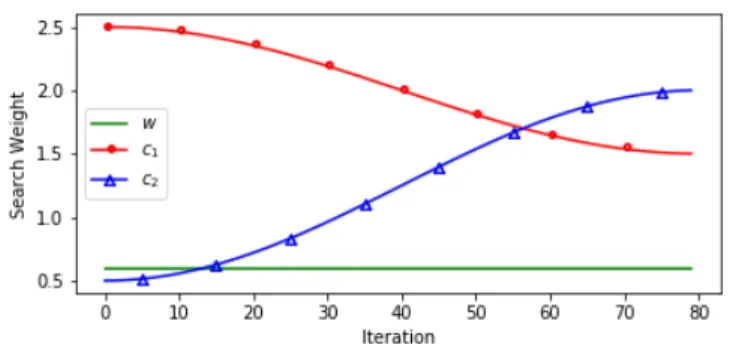
The PSO acceleration coefficientsw, c1, c2 can be seen in (1)

and control the tendency for the particles to follow the previous velocity, their previous personal best position, and the previous overall best position respectively. For this implementation we use the ‘Cosine Late Crossover’ schedule seen in Fig. 1 and consisting of: w= 0.6, (3) c1=q+ Q−q 2 cos(π(1− t T)) + 1 (4)

Fig. 1. Cosine Late Crossover acceleration coefficients

whereq= 1.5,Q= 2.5, and c2=q+ Q−q 2 cos(π t T) + 1 (5)

where q = 0.5, Q = 2.5, which was found in [27] to

provide the best tradeoff between local and global exploration throughout the optimisation/training process. We performed

the optimisation process with a population mof 50 particles

over100 iterations.

C. Parameter Sharing through Lookup Table

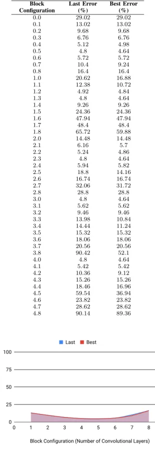
As the joint optimisation and training process progresses, the trained parameters of the models are shared through a lookup table, using a key system to differentiate the weights of each configuration of each individual block in the architecture. An example lookup table following the optimisation process can be seen in Table. I, where the block configuration is

repre-sented by a key following the patterna.b, witha designating

the specific location of the block in the block architecture

model, andb representing the size of the block.

The size of a block (b) determines how many convolutional

layers the block will contain in the generated architecture. It is interesting to note that the performance of each block con-figuration degrades as it moves further away from the optimal configuration found for each block position, with the extreme values often representing very poor results. This can be seen in the increase in error rates for block 1 (the second block of convolutional layers) in the model, where 4 convolutional

layers, identified by the key 1.3 provided the best error rate

of 4.64%, and the error rates consistently increased with an

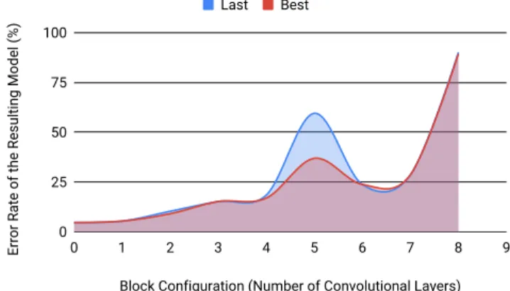
increase or decrease of the block configuration parameter. Visual representations of the lookup table validation error rates can be seen in Fig. 2 for block 0, Fig. 3 for block 1, Fig. 4 for block 2, Fig. 5 for block 3, and Fig. 6 for block 4. The global best result from the optimisation process is therefore represented by the lowest point of each of these graphs, whilst the shape of the graphs suggests that improvements can be found in an area, rather than a single value drastically outperforming all other values.

D. Base Model Preparation

Following the joint optimisation and training process, we diverge from the original SOBA method, which simply chose

(5)

Table. I

EXAMPLELOOKUPTABLECONTENTSFOLLOWINGOPTIMISATION

PROCESS(EVALUATIONPERFOMED ON THEVALIDATIONDATASET)

Block Configuration Last Error (%) Best Error (%) 0.0 29.02 29.02 0.1 13.02 13.02 0.2 9.68 9.68 0.3 6.76 6.76 0.4 5.12 4.98 0.5 4.8 4.64 0.6 5.72 5.72 0.7 10.4 9.24 0.8 16.4 16.4 1.0 20.62 16.88 1.1 12.38 10.72 1.2 4.92 4.84 1.3 4.8 4.64 1.4 9.26 9.26 1.5 24.36 24.36 1.6 47.94 47.94 1.7 48.4 48.4 1.8 65.72 59.88 2.0 14.48 14.48 2.1 6.16 5.7 2.2 5.24 4.86 2.3 4.8 4.64 2.4 5.94 5.82 2.5 18.8 14.16 2.6 16.74 16.74 2.7 32.06 31.72 2.8 28.8 28.8 3.0 4.8 4.64 3.1 5.62 5.62 3.2 9.46 9.46 3.3 13.98 10.84 3.4 14.44 11.24 3.5 15.32 15.32 3.6 18.06 18.06 3.7 20.56 20.56 3.8 90.42 52.1 4.0 4.8 4.64 4.1 5.42 5.42 4.2 10.36 9.12 4.3 15.26 15.26 4.4 18.46 16.96 4.5 59.54 36.94 4.6 23.82 23.82 4.7 28.62 28.62 4.8 90.14 89.36

Block Configuration (Number of Convolutional Layers)

Error Rate of the Resulting Model (%)

0 25 50 75 100 0 1 2 3 4 5 6 7 8 9 Last Best

Fig. 2. Block 0 validation error rate by configuration

0 25 50 75 100 0 1 2 3 4 5 6 7 8 9 Last Best

(6)

0 25 50 75 100 0 1 2 3 4 5 6 7 8 9 Last Best

the global best architecture, finetuned it for a number of epochs on a combined training & validation dataset, and then reported test results. In contrast, we look to utilise multiple particle positions in the swarm in order to promote diversity in the overall resulting model. We experimented with two main methods for choosing candidate base models for the ensemble process, the first method was to use the local best positions from the PSO optimisation process, where the local best represents the best result that each individual particle has previously occupied, which includes the global best. The second method was to use the weight sharing lookup table to nominate particles based on the best results that have been seen for each individual block, in order to promote even more diversity in the resulting base models.

1) Local Best Base Model Nomination: Starting with the

mparticles’ local best positions, we consider only the unique

positions in the search space, as the weight sharing process of the SOBA system ensures that particles with the same position will also have the same parameters, so ensembling them would be relatively pointless. This can be considered as the set of all distinct local best particle positions:

A={Pi}i∈{1,...,n} (6) Which essentially represents every distinct, remaining particle local best, clustered around the global best architecture, where:

Ai= [a1, a2, a3, a4, a5] (7)

This results in a variable number of base models from 1tom

wherem represents the population of the swarm.

2) Lookup Table Base Model Nomination: We also experi-mented with a method to generate candidate base models using

the weight sharing lookup table. By considering each blockBi

in the architecture individually, we check the best values in

the lookup table for each configuration. For each blockBi we

then take two candidate configurations representing the two

best fitness values seen, and construct a tuple (b1, b2) where

bi represents a single integer block configuration. In this way

we build a set of tuples in B, e.g.:

B={(1,2),(1,4),(6,3),(2,7),(0,1)} (8)

which we can then use to generate candidate models by taking the cartesian product of all tuples:

A=B1×· · ·×Bn={(b1, . . . , bn)|xi∈Xi∀i∈ {1, . . . , n}} (9)

This results in 25 or 32 base models using the five-block

skeleton architecture, with an individual model represented by:

Ai = [a1, a2, a3, a4, a5] (10)

e.g. the first model nominated fromB above will be:

A1= [1,1,6,2,0] (11) E. Ensemble Construction

Following the base model nomination process, each individ-ual base model is then individindivid-ually finetuned on a combination dataset consisting of the training dataset and the validation dataset from the optimisation process. This finetuning process

takes the form of an additional 10 epochs of training on

the combined dataset, using a cosine annealing learning rate schedule similar to [28], although we choose not to perform any restarts for this work. None of the parameters of the model are fixed during the finetuning process, it can be considered simply as an extension of the training process for each individual base model. Although notably the parameters learned through this process are not stored in the lookup table.

The learning rate anneals from1e−4down to1e−7over the

10epochs, ensuring that any small improvements in position

can still be made, without jumping over minima. Following the finetuning process, the distinct, finetuned architectures are then combined into an ensemble using a plurality voting

technique (12), where the class D decided for each example

is determined by: D= argmax d∈{1,...,N} T X t=1 Ct,d (12)

where C represents the classifications (Ct,d ∈ {0,1}) of

each base model Ai for each individual class for the input,

d= 1, . . . , N represents the number of classes (N = 10 for

CIFAR-10), and t= 1, . . . , T represents the number of base

models in the base model pool (T = 32 for the lookup table

nomination method). Plurality voting is conceptually similar to majority voting, although in the case where an individual

class for a single example does not achieve more than50% of

the votes, plurality voting still takes the highest voted class, rather than discarding the example as lacking consensus. This technique ensures that we always receive a valid classification for every example, even with widespread confusion amongst the base models.

F. Duplication of Work

A significant downside to the construction of ensembles of deep learning models is the duplication of work that is required in order to generate multiple, distinct models. This duplication of work is common when ensembling CNNs with the same architecture, as often multiple identical models are

(7)

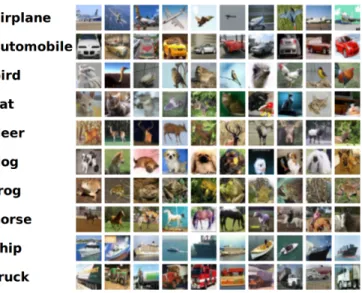
Fig. 7. CIFAR-10 classes with example images

trained either on slices of the dataset with a bagging technique, or even on identical datasets, and then ensembled together to produce a slight increase in performance. Our system alleviates the majority of this duplication of work through our weight sharing mechanism, which ensures that as the optimisation process progresses, the individual blocks in the architectures are trained by all of the models that share them. The only remaining duplication of work is the small finetuning step, whereby we train each base model on the combined training and validation datasets for a small number of epochs in order to reduce overfitting from the optimisation process. This finetuning process takes around four minutes of extra processing time for each base model on our single NVIDIA GTX 1080Ti GPU, representing a very minor increase in required resources.

IV. EVALUATION

We evaluate our system on the CIFAR-10 [29] image

classification dataset, which consists of32×32colour images,

each with a single associated class, examples of which can be seen in Fig. 7. The dataset itself consists of 60,000 images, with precalculated splits of 50,000 for training and 10,000 for testing. We pre-process the images on-the-fly using the augmentations proposed by [30]. For our evaluations we used the same splitting technique as [27], whereby we further split the 50,000 training images into 45,000 training and 5,000 validation. The validation images are then used as the performance measure for the fitness evaluations during the evolutionary optimisation process. After the conclusion of the joint optimisation/training process, the training and validation images were recombined back into the 50,000 image training set which was used to finetune each of base models following the nomination process. To this end, we experimented with the two methods of base model nomination previously described.

A. Local Best Ensemble

Following the conclusion of the joint optimisation and

train-ing process, we were left with 5 distinct local best positions,

with a number of clusters of particles occupying the same position. The finetuning process was performed, taking around

15minutes extra processing time than simply using the global

best position. The final test performance of the individual base models and the resulting constructed ensemble on the CIFAR-10 test set can be seen in Table. II. Each remaining distinct position is given, along with a tally of the number of particles occupying this position at the conclusion of the optimisation process. It’s clear from the results that the global best position provides the best results out of all of our candidate base models. It is also clear that the ensemble technique resulted in improved performance over all of the base models used in

its construction, including an improvement of0.27%over the

global best solution chosen by the optimisation process going

from an error rate of 4.66% down to 4.39%. Fig. 8 shows

each of the remaining, distinct local best positions projected into two dimensions using t-Distributed Stochastic Neighbour Embedding (t-SNE) [31] in order to demonstrate the variations in architecture for the base models in the ensemble.

B. Lookup Table Ensemble

Following the conclusion of the joint optimisation and training process, we used the lookup table base model

nom-ination process described earlier to generate32 base models.

The finetuning process for the lookup based ensemble took

around 2 hours of extra processing time when compared

to simply using the global best. The positions, counts, and test results can be seen in Table. III and Fig. 9 shows the same t-SNE projection for the candidate positions identified by the lookup table method of base-model construction. It is clear that using the lookup table method can provide us with many more diverse candidate base models for ensemble construction than the local best nomination method, although the majority of these models are not necessarily the best candidates overall. Interestingly, the lowest single model error rate was not achieved by the global best position, rather it was achieved by a position that did not appear in the remaining local bests whatsoever. The increased diversity of the base models nominated by the lookup table method resulted in the construction of a much more effective ensemble, producing

an error rate of 4.27%, which was 0.36% lower than the

Table. II

PERFORMANCE MEASURES FOR LOCAL BEST METHOD OF ENSEMBLE CONSTRUCTION ON THECIFAR-10TEST SET

(Integer) Position Particle Tally Accuracy (%) Error Rate (%) [5,3,3,0,0](Global Best) 38 95.34 4.66 [5,2,2,0,0] 4 95.16 4.84 [4,2,3,0,0] 1 95.13 4.87 [5,3,2,0,0] 5 95.29 4.71 [5,2,3,0,0] 2 95.28 4.72 Ensemble N/A 95.61 4.39

(8)

Table. III

PERFORMANCE MEASURES FOR LOOKUP TABLE METHOD OF ENSEMBLE CONSTRUCTION ON THECIFAR-10TEST SET

(Integer) Position Accuracy (%) Error Rate (%) [5,3,3,0,0](Global Best) 95.37 4.63 [5,3,3,0,1] 95.36 4.64 [5,3,3,1,0] 95.42 4.58 [5,3,3,1,1] 95.32 4.68 [5,3,2,0,0] 95.25 4.75 [5,3,2,0,1] 95.30 4.70 [5,3,2,1,0] 95.27 4.73 [5,3,2,1,1] 95.25 4.75 [5,2,3,0,0] 95.27 4.73 [5,2,3,0,1] 95.22 4.78 [5,2,3,1,0] 95.19 4.81 [5,2,3,1,1] 95.23 4.77 [5,2,2,0,0] 95.20 4.80 [5,2,2,0,1] 95.14 4.86 [5,2,2,1,0] 95.12 4.88 [5,2,2,1,1] 95.17 4.83 [4,3,3,0,0] 95.17 4.83 [4,3,3,0,1] 95.05 4.95 [4,3,3,1,0] 95.21 4.79 [4,3,3,1,1] 95.21 4.79 [4,3,2,0,0] 95.14 4.86 [4,3,2,0,1] 95.10 4.90 [4,3,2,1,0] 95.09 4.91 [4,3,2,1,1] 95.09 4.91 [4,2,3,0,0] 95.25 4.75 [4,2,3,0,1] 95.28 4.72 [4,2,3,1,0] 95.11 4.89 [4,2,3,1,1] 95.16 4.84 [4,2,2,0,0] 95.10 4.90 [4,2,2,0,1] 94.99 5.01 [4,2,2,1,0] 95.02 4.98 [4,2,2,1,1] 95.04 4.96 Ensemble 95.73 4.27 [5, 2, 2, 0, 0] [5, 3, 3, 0, 0] [4, 2, 3, 0, 0] [5, 3, 2, 0, 0] [5, 2, 3, 0, 0] t-SNE X t-SNE Y -100 -50 0 50 100 -100 -50 0 50 100

Fig. 8. Projection of the candidate positions identified by the local best method into two-dimensional space using t-SNE (global best in red)

[5, 3, 3, 0, 0] [5, 3, 3, 0, 1] [5, 3, 3, 1, 0] [5, 3, 3, 1, 1] [5, 3, 2, 0, 0] [5, 3, 2, 0, 1] [5, 3, 2, 1, 0] [5, 2, 3, 0, 0] [5, 2, 3, 0, 1] [5, 2, 3, 1, 0] [5, 2, 3, 1, 1] [5, 2, 2, 0, 0] [5, 2, 2, 0, 1] [5, 2, 2, 1, 0] [5, 2, 2, 1, 1] [4, 3, 3, 0, 0] [4, 3, 3, 0, 1] [4, 3, 3, 1, 0] [4, 3, 3, 1, 1] [4, 3, 2, 0, 0] [4, 3, 2, 0, 1] [4, 3, 2, 1, 0] [4, 3, 2, 1, 1] [4, 2, 3, 0, 0] [4, 2, 3, 0, 1] [4, 2, 3, 1, 0] [4, 2, 3, 1, 1] [4, 2, 2, 0, 0] [4, 2, 2, 0, 1] [4, 2, 2, 1, 0] t-SNE X t-SNE Y -100 -50 0 50 100 -100 -50 0 50 100

Fig. 9. Projection of the candidate positions identified by the lookup method into two-dimensional space using t-SNE (global best in red)

global best and0.31% better than the best single base model

performance. C. Overall Results

Table. IV shows a comparison with other, recent evolution-ary architecture generation works, with our model referred to as Swarm Optimsed Block Architecture Ensembles (SOBAE). Notably our method uses a single GPU and runs in a rea-sonable amount of time compared to some of the other works. We also show that with minor increases in the amount of time, using our ensembling method, we can show an improvement of over half a percent when compared to the SOBA [27] method.

V. CONCLUSION

In this paper, we have shown that ensembling through care-ful nomination of base models following a joint evolutionary optimisation and training process for CNN architecture gener-ation can produce improved performance over the single best model found by the search process. We found that constructing and ensembling a pool of base models from our shared weight lookup table could improve the error rate of the resulting

system from4.66%down to4.27%with a two-hour increase

in required processing time. Alternatively, constructing and ensembling a pool of base models from the remaining local best positions following the optimisation process improved the

error rate of the resulting system from4.66%down to 4.39%

with only 15 minutes of extra processing time. Our method

is able to perform the above owing to a minimal duplication of work, as the majority of the training of the base models is performed jointly throughout the optimisation process.

In the future we intend to further explore methods for increasing the diversity of the base models that are generated by the optimisation process, this requires careful thought in order to maintain the structure of the search itself. We also intend to explore different ensembling methods, including weighted ensembling in order to provide more influence to the global best, and the higher performing (better fitness) individuals from the optimisation process.

(9)

Table. IV

CLASSIFICATION RESULTS ONCIFAR-10FOR EVOLUTIONARY ARCHITECTURE OPTIMISATION TECHNIQUES

Method Error Rate (%) GPUs Time (hours) Related Works Large-Scale Evolution [23] 5.40 250 264 Genetic CNN [32] 7.10 ∼20 ∼24 Hierarchical Representations [33] 3.60 200 36 SOBA [27] 4.78 1 34 Ours

SOBAE (local best nomination) 4.39 1 ∼34.25

SOBAE (lookup table nomination) 4.27 1 ∼36

ACKNOWLEDGMENT

This work was supported in part by RPPtv Ltd through an industrial collaborative studentship project.

REFERENCES

[1] A. Krizhevsky, I. Sutskever, and G. E. Hinton, “Imagenet classification with deep convolutional neural networks,” inAdvances in neural infor-mation processing systems, 2012, pp. 1097–1105.

[2] O. Russakovsky, J. Deng, H. Su, J. Krause, S. Satheesh, S. Ma, Z. Huang, A. Karpathy, A. Khosla, M. Bernsteinet al., “Imagenet large scale visual recognition challenge,”International Journal of Computer Vision, vol. 115, no. 3, pp. 211–252, 2015.

[3] P. Kinghorn, L. Zhang, and L. Shao, “Deep learning based image description generation,” inNeural Networks (IJCNN), 2017 International Joint Conference on. IEEE, 2017, pp. 919–926.

[4] B. Fielding, P. Kinghorn, K. Mistry, and L. Zhang, “An enhanced intelligent agent with image description generation,” in International Conference on Intelligent Virtual Agents. Springer, 2016, pp. 110–119. [5] L. Zhang, B. Fielding, P. Kinghorn, and K. Mistry, “A vision enriched intelligent agent with image description generation,” inProceedings of the 2016 International Conference on Autonomous Agents & Multia-gent Systems. International Foundation for Autonomous Agents and Multiagent Systems, 2016, pp. 1488–1490.

[6] S. Antol, A. Agrawal, J. Lu, M. Mitchell, D. Batra, C. Lawrence Zitnick, and D. Parikh, “Vqa: Visual question answering,” in Proceedings of the IEEE international conference on computer vision, 2015, pp. 2425– 2433.

[7] C. Szegedy, W. Liu, Y. Jia, P. Sermanet, S. Reed, D. Anguelov, D. Erhan, V. Vanhoucke, and A. Rabinovich, “Going deeper with convolutions,” inProceedings of the IEEE conference on computer vision and pattern recognition, 2015, pp. 1–9.

[8] C. Szegedy, S. Ioffe, V. Vanhoucke, and A. A. Alemi, “Inception-v4, inception-resnet and the impact of residual connections on learning.” in

AAAI, vol. 4, 2017, p. 12.

[9] S. Singh, D. Hoiem, and D. Forsyth, “Swapout: Learning an ensemble of deep architectures,” in Advances in neural information processing systems, 2016, pp. 28–36.

[10] G. Huang, Y. Li, G. Pleiss, Z. Liu, J. E. Hopcroft, and K. Q. Wein-berger, “Snapshot ensembles: Train 1, get m for free,”arXiv preprint arXiv:1704.00109, 2017.

[11] L. Breiman, “Bagging Predictors,” Machine Learning, vol. 24, no. 2, pp. 123–140, 1996. [Online]. Available: https://doi.org/10.1023/A: 1018054314350

[12] Y. Freund and R. E. Schapire, “A Decision-Theoretic Generalization of On-Line Learning and an Application to Boosting,” Journal of Computer and System Sciences, vol. 55, no. 1, pp. 119–139, 1997. [Online]. Available: http://www.sciencedirect.com/science/article/ pii/S002200009791504X

[13] A. Khatami, M. Babaie, A. Khosravi, H. R. Tizhoosh, and S. Nahavandi, “Parallel deep solutions for image retrieval from imbalanced medical imaging archives,” Applied Soft Computing, vol. 63, pp. 197–205, 2018. [Online]. Available: http://www.sciencedirect.com/science/article/ pii/S1568494617306877

[14] Y. Lecun, L. Bottou, Y. Bengio, and P. Haffner, “Gradient-based learning applied to document recognition,” Proceedings of the IEEE, vol. 86, no. 11, pp. 2278–2324, 1998.

[15] G. Huang, Y. Li, G. Pleiss, Z. Liu, J. E. Hopcroft, and K. Q. Weinberger, “Snapshot Ensembles: Train 1, get M for free,” apr 2017. [Online]. Available: https://arxiv.org/abs/1704.00109

[16] K. Hara, D. Saitoh, and H. Shouno, “Analysis of dropout learning regarded as ensemble learning,” jun 2017. [Online]. Available: https://arxiv.org/abs/1706.06859

[17] G. Huang, Y. Sun, Z. Liu, D. Sedra, and K. Weinberger, “Deep Networks with Stochastic Depth,” mar 2016. [Online]. Available: https://arxiv.org/abs/1603.09382

[18] S. Singh, D. Hoiem, and D. Forsyth, “Swapout: Learning an ensemble of deep architectures,” may 2016. [Online]. Available: http://arxiv.org/abs/1605.06465

[19] L. Zhang, W. Srisukkham, S. C. Neoh, C. P. Lim, and D. Pandit, “Classifier ensemble reduction using a modified firefly algorithm: An empirical evaluation,” Expert Systems with Applications, vol. 93, pp. 395–422, 2018.

[20] M. Galar, A. Fern´andez, E. Barrenechea, and F. Herrera, “EUSBoost: Enhancing ensembles for highly imbalanced data-sets by evolutionary undersampling,”Pattern Recognition, vol. 46, no. 12, pp. 3460–3471, 2013. [Online]. Available: http://www.sciencedirect.com/science/article/ pii/S0031320313002100

[21] E. Bochinski, T. Senst, and T. Sikora, “Hyper-parameter optimization for convolutional neural network committees based on evolutionary al-gorithms,” in2017 IEEE International Conference on Image Processing (ICIP), 2017, pp. 3924–3928.

[22] B. Wang, Y. Sun, B. Xue, and M. Zhang, “Evolving Deep Convolutional Neural Networks by Variable-length Particle Swarm Optimization for Image Classification,” mar 2018. [Online]. Available: https://arxiv.org/abs/1803.06492

[23] E. Real, S. Moore, A. Selle, S. Saxena, Y. L. Suematsu, J. Tan, Q. Le, and A. Kurakin, “Large-Scale Evolution of Image Classifiers,” mar 2017. [Online]. Available: https://arxiv.org/abs/1703.01041

[24] E. Real, A. Aggarwal, Y. Huang, and Q. V. Le, “Regularized Evolution for Image Classifier Architecture Search,” feb 2018. [Online]. Available: http://arxiv.org/abs/1802.01548

[25] J. M. Moyano, E. L. Gibaja, K. J. Cios, and S. Ventura, “An evolutionary approach to build ensembles of multi-label classifiers,”

Information Fusion, 2018. [Online]. Available: http://www.sciencedirect. com/science/article/pii/S1566253518302574

[26] J. Zhao, L. Jiao, S. Xia, V. B. Fernandes, I. Yevseyeva, Y. Zhou, and M. T. Emmerich, “Multiobjective sparse ensemble learning by means of evolutionary algorithms,”Decision Support Systems, 2018.

[27] B. Fielding and L. Zhang, “Evolving image classification architectures with enhanced particle swarm optimisation,”IEEE Access, 2018. [28] I. Loshchilov and F. Hutter, “Sgdr: Stochastic gradient descent with

warm restarts,”arXiv preprint arXiv:1608.03983, 2016.

[29] A. Krizhevsky and G. Hinton, “Learning multiple layers of features from tiny images,” University of Toronto, Toronto, Ontario, Canada, Tech. Rep. vol 1. no. 4, pp. 7, 2009.

[30] K. He, X. Zhang, S. Ren, and J. Sun, “Deep residual learning for image recognition,” inProceedings of the IEEE conference on computer vision and pattern recognition, 2016, pp. 770–778.

[31] L. v. d. Maaten and G. Hinton, “Visualizing data using t-sne,”Journal of machine learning research, vol. 9, no. Nov, pp. 2579–2605, 2008. [32] L. Xie and A. L. Yuille, “Genetic cnn.” inICCV, 2017, pp. 1388–1397. [33] H. Liu, K. Simonyan, O. Vinyals, C. Fernando, and K. Kavukcuoglu, “Hierarchical representations for efficient architecture search,” arXiv preprint arXiv:1711.00436, 2017.