NBER WORKING PAPER SERIES
CORPORATE DEMAND FOR LIQUIDITY
Heitor Almeida Murillo Campello Michael S. Weisbach
Working Paper 9253
http://www.nber.org/papers/w9253
NATIONAL BUREAU OF ECONOMIC RESEARCH 1050 Massachusetts Avenue
Cambridge, MA 02138 October 2002
We thank Viral Acharya, Charlie Hadlock, George Pennacchi and seminar participants at the Atlanta Finance Forum, the University of Illinois, New York University, and the New York Federal Reserve Bank for helpful comments and suggestions. We also thank Steve Kaplan and Luigi Zingales for providing us with their data. The views expressed herein are those of the authors and not necessarily those of the National Bureau of Economic Research.
© 2002 by Heitor Almeida, Murillo Campello and Michael S. Weisbach. All rights reserved. Short sections of text, not to exceed two paragraphs, may be quoted without explicit permission provided that full credit, including © notice, is given to the source.
Corporate Demand for Liquidity
Heitor Almeida, Murillo Campello and Michael S. Weisbach NBER Working Paper No. 9253
October 2002
JEL No. G31, G32, D23, D92
ABSTRACT
This paper proposes a theory of corporate liquidity demand and provides new evidence on corporate cash policies. Firms have access to valuable investment opportunities, but potentially cannot fund them with the use of external finance. Firms that are financially unconstrained can undertake all positive NPV projects regardless of their cash position, so their cash positions are irrelevant. In contrast, firms facing financial constraints have an optimal cash position determined by the value of today’s investments relative to the expected value of future investments. The model predicts that constrained firms will save a positive fraction of incremental cash flows, while unconstrained firms will not. We also consider the impact of Jensen (1986) style overinvestment on the model’s equilibrium, and derive conditions under which overinvestment affects corporate cash policies. We test the model’s implications on a large sample of publicly-traded manufacturing firms over the 1981-2000 period, and find that firms classified as financially constrained save a positive fraction of their cash flows, while firms classified as unconstrained do not. Moreover, constrained firms save a higher fraction of cash inflows during recessions. These results are robust to the use of alternative proxies for financial constraints, and to several changes in the empirical specification. We also find weak evidence consistent with our agency-based model of corporate liquidity.
Heitor Almeida Murillo Campello
Stern School of Business University of Illinois
New York University 340 Wohlers Hall
44 W 4th Street 1206 S. Sixth Street
New York, NY 10012 Champaign, IL 61820
halmeida@stern.nyu.edu m-campe @uiuc.edu
Michael S. Weisbach University of Illinois 340 Wohlers Hall 1206 S. Sixth Street Champaign, IL 61820 and NBER weisbach@uiuc.edu
I
Introduction
One of the most important decisions afinancial manager makes is how liquid afirm’s balance sheet
should be. Given an inflow of cash to thefirm, a manager can choose to reinvest the cash in physical
assets, to distribute the cash to investors, or to keep the cash inside the firm. In fact, managers
choose to hold a substantial portion of their assets in the form of cash and liquid securities; in 1999, for the 25 nonfinancial companies in the Dow Jones index, the average ratio of cash and equivalent securities to annual capital expenditures was 227%, and for 11 of the 25 the ratio was at least
97%. The financial press has been critical of these large cash holdings, and suggests that they are
a manifestation of agency problems.1 However, the difficulty with these sorts of criticisms is that
they are made without a sense of what cash holdings would be in the absence of agency problems. As Keynes (1936) originally discussed, the major advantage of a liquid balance sheet is that it
allows firms to make value-increasing investments when they occur. However, Keynes also pointed
out that this advantage is limited by the extent to which firms have access to capital markets (p.
196). We present a model that formalizes this intuition. In it, afirm whose access to capital markets
is limited by the nature of its assets, may anticipate facingfinancing constraints when undertaking
investments in the future. Cash holdings are valuable because they increase the likelihood that the firm will be able to fund those investments. However, increasing cash is also costly for such a firm because it decreases the quantity of current investments that the firm can make. In other
words, cash yields a lower return than that associated with thefirm’s physical investments precisely
because thefirm foregoes current positive NPV projects in order to hold cash. In contrast to afirm
facing constrained access to the capital markets, an unconstrained firm (i.e., afirm that is able to
invest in all of its positive NPV projects) has no use for cash, but also faces no cost of holding cash. Our model contains a number of empirical predictions for corporate cash policies. The cleanest
of those predictions concerns a firm’s propensity to save cash out of cash inflows, which we refer
to as the cash flow sensitivity of cash. Our model implies that a firm’s cash flow sensitivity of
cash depends on the extent to which thefirm faces financing constraints: firms that arefinancially
unconstrained should not have a systematic propensity to save cash, whilefirms that are constrained
should have a positive cashflow sensitivity of cash. We also study whether these optimal cash policy
1See, for example, “What to do with all that cash?”, Business Week, Nov/20/2000, and “Time pressure on six
implications remain when the firm can hedge against future cashflows. In a framework similar to that of Froot et al. (1993), we analyze both hedging and cash policies. Unlike these authors, we
assume that the same frictions that make firmsfinancially constrained also constrain their ability
to hedge. Although the analysis of cash policies becomes more involved when firms are allowed to
hedge, the main implications of our model continue to hold.
We also study the implications of agency arguments such as Jensen (1986) in the context of our model. We do so because of the common view that large cash positions are a manifestation of agency problems, and also because evidence from Blanchard et al. (1994), Harford (1999), and Lie (2000) suggests that incremental cash is likely to be used on value-reducing investments, consistent with the story that managers’ utilities are increasing with the quantity of thefirm’s assets. Accordingly,
we model a situation in which an overinvestment-prone manager potentially distorts hisfirm’s cash
policies. Because the manager derives utility from reducing investments in addition to
value-increasing ones, he will save a portion of cash inflows to the firm that can exceed the amount of
savings needed to fund thefirst-best level of investment. Such policies ensure the manager’s ability
to undertake all the investments he desires in the future, even if he does not have access to capital markets. Perhaps the most interesting implication of the agency model of liquidity is that the
effect of overinvestment tendencies on firm’s cash policies will be most pronounced for firms that
are relatively unconstrained in the capital markets, but which do not have sufficient free cashflow
to fund the manager’s desired investment. Intuitively, the agency problem turns afirm that would
be unconstrained if it invested at thefirst best level into one that is effectively constrained because of the extra investment its manager would like to undertake.
We evaluate the implications of our theory on a sample of manufacturing firms between 1981
and 2000. Because the main predictions of our model concern differences between constrained
and unconstrained firms, we classify firms by the nature of their financial constraints using five
alternative approaches suggested by the literature. For each classification scheme, we estimate the cash flow sensitivity of cash for both the constrained and the unconstrained firm subsamples. We find that, under each of thefive classification schemes, the cash flow sensitivity of cash is close to
and not statistically different from zero for the unconstrained firms, but positive and significantly
different from zero for the constrainedfirms. Thisfinding is consistent with the implications of our
behavior offirms’ propensity to save cash out of cash inflows over the business cycle. We find that
the cash flow sensitivity of cash of financially constrained firms is negatively associated with the
level of aggregate demand (i.e., constrainedfirms save more in recessions), while unconstrainedfirms display no change in their cash policies over the cycle. Our model is consistent with this pattern of
changes in liquidity demand over the business cycle because aggregate demandfluctuations work as
exogenous shocks affecting both the size of current cashflows as well as the relative attractiveness
of current investment vis-a-vis future investment.
We also empirically assess the extent to which agency considerations affect the decision to retain cashflows. To do so, we follow much of the literature in presuming that stock ownership and options
help improve managers’ incentives. Given this assumption, our model implies that the cash flow
sensitivity of cash should be related to managerial compensation packages, but only for thosefirms
that: a) have easy access to capital markets, and b) do not have large stockpiles of cash (“free cash flow”). We find that the extent to which this relationship is supported in the data depends
on the measure offinancial constraints we use. When we use dividend policy and size to measure
financial constraints, the coefficient on cash flow interacted with ownership of stock and options is
negative and statically significant for financially unconstrained firms with low free cash flow, and
not significant for all other firms. These results are consistent with our theory, and suggest that
financially unconstrained firms whose managers are likely to have little or no incentives to adopt
value-maximizing policies seem to manage firm liquidity as if they were financially constrained.
The results are less compelling, however, when we use alternative measures offinancial constraints
(such as bond and commercial paper ratings). In all, we interpret these findings as providing at
least weak evidence that agency problems at the margin can induce managers to hold excessive
cash, which accords with our agency view of liquidity.2
We are by no means the first ones to consider the issue of corporate liquidity and its effects
on investment. Besides Keynes (1936), the idea thatfirms may underinvest because of insufficient
liquidity and imperfect capital markets has been considered in several classic papers in the corporate finance literature, such as Jensen and Meckling (1976), Myers (1977), and Myers and Majluf (1984). More recently, Kim et al. (1998) present a model of cash holdings forfirms which face costly external financing. In their model, firms trade offan (exogenously assumed) lower return of holding liquid
2
assets and the benefit of relaxingfinancial constraints in the future. They use their model to derive
implications for the optimal level of cash holdings, arguing that firms which face higher costs of
external funds and have higher variance in future cashflows should hold more cash.3
A number of recent empirical studies examine the cross-section of cash reserves, and the factors
that appear to be associated with higher holdings of cash.4 These papers find that the levels
of cash tend to be positively associated with future investment opportunities, business risk, and
negatively associated with proxies for the cost of externalfinance and with the level of protection
of outside investors. While these studies focus on differences in the level of cash acrossfirms, our
paper examines differences in thesensitivity of cash holdings to incremental changes in cash flow,
and the extent to which they are affected by the firm’s financial status. We do so because our
analysis suggests that the theory has much clearer predictions aboutfirms’ marginal propensity to
save/disburse out of cashflow innovations than about the amount of cash in their balance sheets.5
The remainder of the paper proceeds as follows. Section II introduces a theory of corporate liquidity demand. Section III presents the empirical tests of our theory’s main implications. Section IV is a brief conclusion.
II
A Simple Theory of Liquidity Demand
A
The Basic Model: Cash as a Storage Technology
Thefirst step of our analysis is to model corporate demand for liquid assets as a means of ensuring the ability to invest in the future. In an imperfect capital market, saving for future expendi-tures might be valuable if thefirm anticipates rising financing costs or if thefirm anticipates that the future investment opportunities will be particularly profitable. Our basic model is a simple
representation of a dynamic problem in which the firm has both present and future investment
opportunities. The key feature of the model is that cash flows from current assets might not be
3Other related papers are John (1993), who studies the link between liquidity andfinancial distress costs, Baskin
(1987), who examines the strategic value of cash in games of product-market competition, and Acharya et al. (2002), who consider the effect of optimal cash policies on corporate credit spreads.
4
An incomplete list of papers includes Kim et. al. (1998), Opler et al. (1999), Pinkowitz and Williamson (2001), Faulkender (2002), Ozkan and Ozkan (2002), and Dittmar et al. (2002). Opler et al. further examine the persistence of cash holdings, and characterize whatfirms do with “excess” cash.
5
The strategy of analyzing corporate policies by looking at cross-sectional differences in cashflow sensitivities has been used in the empirical literature largely initiated by Fazzari et al. (1988). While that literature has focused on corporate policies such as working capital (Fazzari and Petersen (1993) and Calomiris et al. (1995)), and inventory demand (Carpenter et al. (1994) and Kashyap et al. (1994)), it has remained silent on the issue of liquidity demand.
sufficient to fund all positive NPV projects, in the present and in the future. Hoarding cash may
therefore facilitate future investments. Of course, another way thefirm can plan for the funding of
future investments is by hedging against future earnings. Alternatively, the firm may also adjust
its dividend policies or its borrowing. In all, our framework considers four components offinancial
policy: liquidity management, hedging, dividend payments, and borrowing. A.1 Structure
The model has three dates, 0, 1, and 2. At time 0, the firm is an ongoing concern whose cash
flow from current operations is c0. At that date, the firm has the option to invest in a long term
project that requiresI0 today and pays offF(I0) at time 2. Additionally, thefirm expects to have
access to another investment opportunity at time 1. If thefirm investsI1 at time 1, the technology
produces G(I1) at time 2. The production functions F(·) and G(·) have standard properties, i.e.,
are increasing, concave, and continuously differentiable. The firm also has existing assets which
will produce a cashflow equal to c1 in period 1. With probability p, the time 1 cash flow is high,
equal tocH1 , and with probability(1−p), equal tocL1 < cH1 . We assume that the discount rate is 1,
everyone is risk neutral, and the cost of investment goods equals 1. Finally, the investmentsI0 and
I1 can be liquidated at thefinal date, generating a payoffequal toq(I0+I1),where we assume that
q <1. Define the total cashflows from investments asf(I0)≡F(I0) +qI0,andg(I1)≡G(I1) +qI1.
We suppose that the cash flows F(I0) and G(I1) from the new investments are not verifiable.
While the firm cannot pledge those cashflows to outside investors, it can raise externalfinance by
pledging the underlying productive assets as collateral. Following Hart and Moore (1994), the idea is that the liquidation value of “hard” assets is verifiable and if thefirm reneges on its debt creditors will seize the physical assets. Assume that the liquidation value of those assets that can be captured by creditors is given by (1−τ)qI. τ ∈(0,1)is a function of factors such as asset tangibility, and the legal environment that dictates the relations between debtors and creditors (see Myers and Rajan (1998)). This parameter is an important element of our theory in that we want to separate
the behavior of firms which are financially constrained – and thus need to rely more on cash as
a storage technology – from financially unconstrained firms. Clearly, for a high enough τ, the
constrained.6 In this set up, the firm is only concerned about whether to store cash from time 0
until time 1 as there is no new investment opportunity at time 2. We denote byC the amount of
cash the firm chooses to carry from date 0 to date 1.7 We assume thatI0,I1>0.
As a benchmark case, we solve for the optimal cash policy when the firm can fully hedge future
earnings. However, consistent with our assumptions about income contractibility, we also analyze the more interesting situation in which only a fraction (1−µ) of future earnings can be costlessly pledged to external investors. In this case, thefirm cannot credibly sign a contract in which it pays
more than (1−µ)cH1 in the high state.8 Under this richer environment, the underlying source of
incomplete contractibility (reflected in both τ and µ) caps the firm’s ability to transfer resources
both across time and across states.9
A.2 Analysis
When the interests of managers and shareholders converge, the objective is to maximize the
ex-pected lifetime sum of all dividends subject to several budget andfinancial constraints. Thefirm’s
problem can be written as
max C,h,I ¡ d0+pdH1 + (1−p)d1L+pdH2 + (1−p)dL2 ¢ s.t. (1) 6
In the Hart and Moore framework the optimal contract is most easily interpreted as collateralized debt. Our conclusions, though, do not hinge on any particular element of that framework. So long as constrainedfirms have limited capacity to issue equity (or if equity issues entail deadweight costs) our theory’s intuition will still hold. An alternative framework that allows for equity finance is the moral hazard model of Holmstrom and Tirole (1997), where it is not optimal forfirms to issue equity beyond a certain threshold due to private benefits of control.
7In principle,C can be negative as thefirm may not only carry no cash from time 0 to time 1, but also borrow
against future earningsc1. For practical purposes, one can think ofCas a positive quantity. However, we will later
show that our main predictions about cashflow sensitivities of cash do not depend onCbeing necessarily positive.
8
To see how the hedging technology works, consider the case where cL1 = 0. Suppose thefirm has the same
investment opportunities in both states (LandH) at time 1. Because borrowing capacity is limited, thefirm might wish to transfer cash flows to state L. This can be accomplished, for example, by selling futures contracts on the asset that produces the time 1 cashflow. In a frictionless world, thefirm would be able to fully hedge by selling that asset’s entire stream of cashflows in the futures market at time 0 and thefirm would have locked in a payoffofpcH1
in both states. However, since the amountµcH1 of cash flows is not contractible, thefirm always has the option of
walking away withµcH
1 in stateH. Thus, a perfectly hedged position through the use of futures contracts can only
happen ifµcH1 ≤pcH1 . If on the other handµ > p, then the hedging policy of thefirm will be constrained.
9One could think ofτ (theborrowing constraint) andµ(thehedging constraint) as highly correlated. In fact, our
analysis would yield similar results if we assumed they are equal. We, however, denote those parameters differently so that the effects of hedging on cash policies are made clear in the analysis.
d0 = c0+B0−I0−C≥0 dS1 = cS1 +hS+B1S−I1S+C≥0, forS =H, L dS2 = f(I0) +g(I1S)−B0−B1S, forS =H, L B0 ≤ (1−τ)qI0 B1S ≤ (1−τ)qI1S, forS =H, L phH+ (1−p)hL = 0 −hH ≤ (1−µ)cH1
The first two constraints restrict dividends (d) to be non-negative in periods 0 and 1. B0 and
B1 are the amounts of collateralized borrowing. Debt obligations are repaid at the time when the
assets they helpfinance generate cashflows, and their face values are constrained by the liquidation
value of those assets.10 hH and hL are the hedging payments. The hedging strategies we focus on
typically givehH <0andhL>0. If thefirm uses futures contracts, for example, we should think of
cS1+hSas the futures payoffin stateS. Thefirm sells futures at a price equal to the expected future
spot value, and thus increases cashflows in state L at the expense of reducing cashflows in state
H. If the hedge ratio is equal to 1, then thefirm is fully hedged andcH1 +hH=c1L+hL=E0[c1].
When thefirm faces capital market imperfections not all future cashflows can be used for hedging
purposes, and the hedge ratio may be less than 1. Finally, note that the fair hedging constraint phH+ (1−p)hL= 0defineshH as a function ofhL:
hH= (p−1)
p h
L.
We refer to hH as thefirm’s “hedging policy”. This policy is constrained by the fact that thefirm
cannot commit to pay out more than (1−µ)cH
1 in stateH.
A.2.1 First best solution Thefirm isfinancially unconstrained if it is able to invest at thefirst best levels. The first best investment levels at times 0 and 1 (I0F B and I1F B) are defined by:
f0(I0F B) = 1
g0(I1F B,S) = 1, forS=H, L.
1 0This formulation implies that ourfinancial constraint is a quantity constraint. Alternatively, we could study a
model in whichfirms face an increasing (deadweight) cost of externalfinance. As we will argue later, in our analysis all constrainedfirms have a similar propensity to save cash (irrespective of how tight the constraint is), suggesting that our results do not hinge on the formulation based on quantities.
When the firm is unconstrained its investment policy satisfies all the dividend, hedging, and bor-rowing constraints above for some financial policy (B0, B1S, C, hH). Except for a case when the
constraints are exactly binding at the first best solution, the financial policy of an unconstrained
firm will not matter. In particular, if afirmj isfinancially unconstrained, then itsfinancial policy
(B0j, B1j, Cj, hHj )can be replaced by an entirely differentfinancial policy( ˆB0j,Bˆ1j,Cˆj,hˆHj )with no
implications forfirm value. Consequently, there is no optimal cash hoarding policy for afinancially
unconstrained firm. To see the intuition, suppose the firm increases its cash holdings by a small
amount ∆C. Would that policy entail any costs? The answer is no. The firm can compensate for
∆C by paying a smaller dividend today. Are there benefits to the increase in cash holdings? The
answer is also no. The firm is already investing at thefirst best level at time 1, and an increase in
cash is a zero NPV project since thefirm foregoes paying a dividend today for a dividend tomorrow
that is discounted at the market rate of return.
A.2.2 Constrained solution In the context of our model, it is easy to operationalize the
no-tion of financial constraints; in particular, we define a firm to be financially constrained if its
investment policy is distorted from the first-best because of capital market frictions, i.e., if (I0∗, I1∗)<(I0F B, I1F B). For a financially constrainedfirm, holding cash entails both costs and benefits. A financially constrained firm cannot undertake all of its positive NPV projects, so holding cash is costly because it requires sacrificing some valuable investment projects today. The benefits of
cash occur because it allows thefirm tofinance future projects that might arise. Firms will choose
cash holdings to trade off these costs and benefits of cash, both of which are generated by the
same underlying reason (capital market imperfections). As a result of these countervailing effects, financial constraints will give rise to an optimal cash policy C∗. This is in stark contrast with the “irrelevance of liquidity” result that holds forfinancially unconstrainedfirms.
In order to characterize the optimal cash holding of a constrained firm we have to determine
the optimal investment and financial policies of that firm. If the firm is financially constrained,
it will not be optimal to pay any dividends at times 0 and 1. Furthermore, borrowing capacity will be exhausted in both periods and in both states at time 1. This must be the case, since foregoing a dividend payment or borrowing an additional unit is a zero NPV project, and, recall,
optimization problem as follows:11 max C,hLf µ c0−C 1−q+τ q ¶ +pg à cH1 −1−pphL+C 1−q+τ q ! + (1−p)g µ cL1 +hL+C 1−q+τ q ¶ s.t. (2) hL≤(1−µ) p 1−pc H 1
Notice that we have collapsed the fair hedging condition and the hedging constraint into one
equation. Moreover, note that the hedging constraint hL ≤ (1−µ)1−ppcH1 need not bind. This
happens, for example, when the firm can transfer enough cash flows to state L such that there
is no constrained hedging demand. Now the firm’s problem reduces to an optimization in C and
hL, constrained by the maximum hedging available. As suggested above, we consider solving this
problem both with and without hedging constraints. To economize on notation, defineλ≡1−q+τ q.
Unconstrained hedging: Suppose the hedging constraint does not bind. Because hedging
is fairly priced the firm can eliminate its cash flow risk. This implies that the optimal amount of
hedging is given byhL=p(cH1 −c1L), which gives similar cashflows in both states (equal toE0[c1]).12
It is easy to see that the hedging constraint will not bind so long as(1−p)(cH1 −c1L)≤(1−µ)cH1 . If the optimal hedge is feasible, the optimal cash policy will be determined by:
f0 µ c0−C λ ¶ =g0 µ E0[c1] +C λ ¶ (3)
The left-hand side of Eq. (3) is the marginal cost of increasing cash holdings. If the firm hoards
cash it sacrifices valuable (positive NPV) current investment opportunities.13 The right-hand side
of Eq. (3) is the marginal benefit of hoarding cash under financial constraints. By holding more
cash the firm is able to relax the constraints on its ability to invest in the future.
How much of its current cashflow will a constrainedfirm save? This can be calculated from the
derivative ∂c∂C
0, which we define as thecashflow sensitivity of cash. As we illustrate below, the cash flow sensitivity of cash is a very useful concept in that it reveals a dimension of corporate liquidity
policy that is suitable for empirical analysis. The interpretation resembles that of the cash flow
sensitivity of investment used in thefinancial constraint literature (Fazzari et al. (1988)). 1 1We replace the binding constraints in the objective function and eliminate the terms that are constant. 1 2
This is just a traditional “full-insurance” result. In order to check it, one can take the derivative of the objective function with respect tohLand set it equal to zero.
1 3These opportunities are valuable precisely becausefinancial constraints force the marginal productivity of
The cashflow sensitivity of cash is given by: ∂C
∂c0
= f00(I0)
f00(I0) +g00(I1) >0
This sensitivity is positive, indicating that if afinancially constrainedfirm gets a positive cashflow innovation this period, it will optimally allocate the extra cash across time, saving some resources for future investments.
Importantly, note that the optimal cash holdings bear no obvious relationship with borrowing
capacity (the parameterτ). This can be seen by examining the derivative:
∂C ∂τ =
−q(c0−C)f00(I0) +q(E0[c1] +C)g00(I1)
τ(f00(I0) +g00(I1)) ,
which cannot be signed. The intuition is that higher debt capacity relaxes financial constraints
both today and in the future, yielding a similar effect on the marginal value of cash across time.
An Example: A simple example can show in a more intuitive way the empirically testable
impli-cations of our model. Consider parametrizing the production functionsf(·) andg(·)as follows: f(x) =Aln(x) and g(y) =Bln(y) (4)
This parametrization assumes that while the concavity of the production function is the same in
periods 0 and 1, the marginal productivity of investment may change over time.14 With these
restrictions, it is a straightforward task to derive an explicit formula for C: C∗ = δc0−E0[c1]
1 +δ , (5)
whereδ ≡ BA >0. The cash flow sensitivity of cash is then given by 1+δδ ,15 where the parameterδ can be interpreted as a measure of the importance of future growth opportunities vis-a-vis current opportunities. Eq. (5) shows thatCis increasing inδ(i.e., ∂C∂δ >0), which agrees with the intuition
that a financially constrained firm will hoard more cash today if future investment opportunities
are more profitable. Note also that cashflow sensitivity of cash, given by 1+δδ ,is independent of the
parameter τ. Since the optimal cash policy is determined by an intertemporal trade-off, a change
1 4
Similar results will hold for a more general Cobb-Douglas specification for the production function, namely
f(x) =Axα andg(x) =Bxα.The important assumption is that the degree of concavity of the functions f andgis the same. Given this, the particular value ofαis immaterial. We use theln(·)specification because it simplifies the algebra and economizes on notation.
1 5Notice that the sensitivity does not depend on whether the cash balanceC∗is positive or negative. Eq. (5) also
in borrowing capacity does not matter if the firm is already constrained. This analysis in turn
establishes a precise and monotonic empirical relationship between financial constraints and the
cashflow sensitivity of cash: constrained firms should display positive cash—cashflow sensitivities,
while unconstrained firms should not have a systematic propensity to save cash. For the purpose
of empirical testing, the degree of the financial constraints will not matter for alreadyconstrained
firms.16 Thus, the issue of non-monotonicity in the relationship betweenfinancial constraints and cash policies is not a first-order concern for empirical analysis in this context.17 We explore these properties of our theory in the tests of Section III.
Constrained hedging: If the hedging constraint binds, the amount of hedging is given by hL= (1−µ)1−ppcH1 . In this case, the optimal cash policy is determined by:
max C f µ c0−C λ ¶ +pg µ µcH1 +C λ ¶ + (1−p)g à cL1 + (1−µ)1−ppcH1 +C λ ! (6) or f0 µ c0−C λ ¶ =E0[g0(I1)]. (7)
The only difference from the previous Eq. (3) is that marginal productivity now varies across states because of the constraint on hedging. The comparative statics are more involved with constrained hedging, but our previous results remain. In the appendix, we use our previous parametrization to
derive the following results for hedge-constrainedfirms:
• If time0cashflow increases, then thefirm hoards more cash (i.e., the cashflow sensitivity of cash is positive):
∂C ∂c0
>0
• If future investment opportunities are more profitable than the current investment
opportu-nities (δ is high), then thefirm hoards more cash: ∂C
∂δ >0
1 6Notice that the cashflow sensitivity of cash is similar for all constrainedfirms, irrespective of how constrained
they are. This suggests that our conclusions do not hinge on our formulation of financial constraints as quantity constraints. If thefinancial constraint manifests itself in terms of increasing costs of externalfinance, a change in the cost would relax constraints by a similar amount today and in the future, generating very similar implications.
1 7
This result is important because it essentially avoids the theoretical critique advanced by Kaplan and Zingales (1997, 2000) regarding the traditional interpretation of investment-cashflow sensitivities. See also the discussion in Fazzari et al. (2000), Povel and Raith (2001), and Almeida and Campello (2002).
Also similarly to the case of perfect hedging, borrowing capacity will not affect cash policies for firms which are constrained. However, we now have an additional implication related to changes in the hedging constraint:
• Firms which can hedge less hoard more cash:
∂C ∂µ >0
The intuition for this last result is as follows. The cost of limited hedging is the difference in the marginal value of funds across states in the future. The marginal value is higher in the state where thefirm has lower cashflows. An increase inµ increases funds in state H,but decreases funds in
state L.This increases the difference in the marginal value of funds across states, and causes the
firm to increase cash hoarding so as to rebalance the future marginal value in the two states. In sum, the main implications of the basic model are still true when hedging is constrained. While there is no optimal cash policy if thefirm isfinancially unconstrained, the cashflow sensitivity of cash is positive for constrainedfirms. Moreover, conditional on the fact that afirm isfinancially constrained, borrowing capacity has no additional effect on the optimal cash policy. Thus, cash flow sensitivities of cash should be monotonically increasing infinancial constraints. We state this result in the form of a proposition.
Proposition 1 The cash flow sensitivity of cash offinancially unconstrained and financially con-strained firms have the following properties:
∂C ∂c0
= 0 for financially unconstrained firms (8) ∂C
∂c0
> 0 for financially constrained firms
This is the main implication of the basic model that we test in the empirical section below.18
Two additional implications of the model are that constrainedfirms should hoard more cash if they
have more valuable future investment opportunities, and that cash and hedging are substitutes for firms that are hedge-constrained. While we can empirically examine thefirst of these two additional implications, data availability precludes us from studying the latter implication in this paper.
1 8
To be precise, when we say that ∂C
∂c0 = 0 for financially unconstrained firms we do not mean to say that the
sensitivity must be always equal to zero in an economic sense. Rather, we imply that the cash policy of unconstrained firms is undetermined, and thus their cashflow sensitivity should not bestatisticallydifferent from zero.
B
Agency Problems: Overinvestment Tendencies
Any model in which those in charge of running the day-to-day operations of the firm (managers)
have objectives that are different from those who own the firm (shareholders) can be seen as an
agency model. For practical purposes, the more interesting types of agency problems are those in which managers take actions that reduce shareholders’ wealth. Within this class of problems, most
of the research in corporatefinance has investigated one type of agency problem: the overinvestment
problem (see Stein (2001) for a review). In this subsection, we build on our basic model of liquidity demand and study how overinvestment-prone managers handle corporate liquidity.
There are alternative ways of modeling managers’ tendency towards overinvestment. As in Hart and Moore (1995), we analyze a model in which managers enjoy private benefits that increase with a firm’s investment. This assumption is plausible because executives’ salaries are typically increasing infirm size, and because non-pecuniary benefits of control are likely to be more valuable in larger firms. Implicitly, we are assuming that no feasible incentive contract, corporate governance system, or other external threats can make managers internalize the full value consequences of inefficient investment decisions (see Jensen (1993) or Stein (2001) for more discussion).
A very simple way to introduce this type agency problem in our model is to assume that
managers make investment andfinancing decisions so as to maximize the following utility function:
UM = (1 +θ)£f(I0) +pg(I1H) + (1−p)g(I1L) ¤
,whereθ≥0, (9)
whereθis interpreted as a measure of the residual amount of agency problems which remains after
all feasible corrective mechanisms have been applied.19 Notice that the maximization program of
the previous subsection (Eq. (1)) is naturally nested in Eq. (9). In other words, our basic model is
a special case of Eq. (9) which obtains when there is no overinvestment problem (i.e., whenθ= 0).
It is straightforward to verify that the particular agency problem we consider – a tendency to overinvest – has nofirst-order effect on the cash policy offinancially constrainedfirms. Intuitively, 1 9We borrow this formulation from Stein (2001) for ease of exposition. This is equivalent to assuming that managers
apply the following transformation to the investment functionsf(·)andg(·):
fM(x) = (1 +θ)f(x)
gM(x) = (1 +θ)g(x)
A broader class of utilities would also lead to our main conclusions about cash management in the presence of overinvestment tendencies.
a positiveθuniformly raises the marginal productivity of all investment opportunities (current and
future), thus the trade-offwhich determines optimal cash is the same irrespective of the value ofθ.
The more interesting result on the influence of agency on cash management happens when the firm is financially unconstrained. For a large θ, an unconstrained firm will behave as if it were financially constrained. Intuitively, even when capital markets are perfect, investors will only be
willing to give funds to the firm up to a limit determined by the true payoff from investment.
Consequently, there exists an “optimal” financial policy of afirm controlled by an
overinvestment-prone manager, similarly to what we predict for a financially constrainedfirm.
In order to see this result, notice that we can write the program solved by afirm facing perfect
capital markets that is subject to agency problems as:
max C,I,hL(1 +θ)f(I0)−B0+p[(1 +θ)g(I H 1 )−BH1 ] + (1−p)[(1 +θ)g(I1L)−B1L]s.t. (10) I0 = c0+B0−C I1S = cS1 +hS+B1S+C, for S=H, L B0 ≤ f(I0) B1S ≤ g(I1S) forS =H, L 1−p p h L ≤ (1−µ)cH1
The firm can borrow up to the true value of the investments I0 and I1. Recall, the functions f(·)
and g(·) include the cash flows from liquidationqI0 and qI1.And we are implicitly setting τ = 1,
consistent with the idea that the firm faces perfect capital markets. Clearly, if θ = 0, the firm
would invest at thefirst best levels and would not have a systematic cash policy.20 Let us in turn
solve for the optimal investment and cash policies whenθ >0.
If managers are able to (over)invest as much as they wish, they would choose the levels of investment to satisfy:
f0(Ib0) =g0(Ib1) =
1
1 +θ <1. 2 0Notice that profit maximization implies that ifIF B
0 >0:
f(I0F B)≥I
F B
0
The question is whether managers can finance these levels of investment. Consider the case of
unconstrained hedging. We can assume with no loss of generality that thefirm will have the same
cashflow in both states at date 1 (equal to E0[c1]). Now the condition guaranteeing that thefirm
is able tofinance the investment levelsIb0 and Ib1 is that there exists a level of cash Cb such that: b
I0 ≤ c0+f(Ib0)−Cb b
I1 ≤ E0[c1] +f(Ib1) +Cb
Summing the two equations we obtain the condition:
b
I0−f(Ib0) +Ib1−f(Ib1)≤c0+E0[c1] (11)
The left hand-side of (11) is the negative NPV generated by the projects at the super-optimal scales of production.21 The right hand-side can be interpreted as thefirm’s “free cashflow”, or total free resources available for investment. Since there is a tendency for overinvestment, shareholder
wealth is decreasing in the amount offirm’s free cashflows (Jensen (1986)). The expression simply
says that overinvestment will be limited by the availability of cash from current operations (c0 and
E0[c1]). Free cash flow will enable mangers to invest in negative NPV projects even when the
market is not willing to finance those projects.
The overinvestment-prone firm will have a uniquely defined cash policy only if Ib0 −f(Ib0) + b
I1 −f(Ib1) > c0+E0[c1], that is, if total resources available for investment are not too large. If
condition (11) is met, then there are multiple cash policies Cb which allow the firm to invest at
the super-optimal levels (unless the condition is satisfied with an exact equality). Similarly to financially unconstrainedfirms which invest optimally, thesefirms do not have a well-defined cash
policy. In other words, if these firms receive an additional cash inflow (i.e., c0 goes up), it is a
matter of indifference to suchfirms whether they save the additional cash or pay dividends.
If condition (11) is not obeyed then thefirm behaves as if it were a financially constrainedfirm.
The borrowing constraints will be binding, and the firm will choose optimal cash and investment
policies according to:
max
C,I0, I1
θf(I0) +θg(I1) s.t.
2 1It is possible that the investment projects are still positive NPV, even at the super-optimal scale. In this model,
only the marginal investments aboveIF B are necessarily negative NPV. The total NPV of the investmentIbmay be positive or negative. If it is positive, then thefirm can always overinvest in this model. However, if the difference betweenIbandIF B is high enough then the total NPV should also be negative.
I0 = c0+f(I0)−C
I1 = E0[c1] +g(I1) +C
The only difference with respect to the constrainedfirm’s optimization problem (recall Eq. (2))
is that since the borrowing constraints are not linear in investment we cannot solve the constraints
explicitly for I0 and I1. The intuition, though, is the same. The optimal cash balance C∗ is
determined so as to equate the marginal productivity of investment at the two dates (note that θ
will not matter for this choice):
f0[I0(C∗, c0)] =g0[I1(C∗)]
where I0(C∗, c0) and I1(C∗) represent the optimal investment levels (I0∗, I1∗) as functions of cash
and cash flows.22 It is easy to show that the cashflow sensitivity of cash is positive. Noting that
∂I0
∂c0 >0,
∂I0
∂C < 0 and ∂I1
∂C > 0, differentiating the fist order condition allows us to write the cash
flow sensitivity of cash as:
∂C∗ ∂c0 = f 00(I0)∂I0 ∂c0 g00(I1)∂I1 ∂C −f00(I0) ∂I0 ∂C >0
Our analysis formalizes Jensen’s (1986) argument about managerial overinvestment tendencies: firms with plenty of free resources in hand (high c0, E0[c1]) will invest at the level Ibt, whilefirms
with less resources will only be able to invest at the lower level, It∗, which is more desirable from the perspective of shareholders – i.e., it is closer to the first best investment level.23
This analysis has testable implications for the effect of overinvestment on cash policies. If afirm is underinvesting because of limited access to the capital markets (i.e., is financially constrained), then overinvestment tendencies have no distinct effect on cash policies in general, and on the cash flow sensitivity of cash in particular. This is because overinvestment does not affect a constrained firm’s trade-off between foregoing investment opportunities today and increasing investment
to-morrow. Tests of the overinvestment hypothesis should thus focus on firms with good access to
external funds. But notice that in order for overinvestment to have an effect on cash policies, it
is also necessary that the firm does not have too much internal resources (free cash flow). If one
2 2
Investment levels are determined directly from the binding constraints:
I0∗ = c0+f(I0∗)−C∗
I1∗ = E0[c1] +g(I1∗) +C∗
2 3Notice thatIF B
t < It∗<Ibt, witht= 1,2.Thefirst inequality is true because the constraints cannot be binding for investment levels lower thanItF B, and the second follows from the condition in Eq.(11).
is able to empirically identify suchfirms, then the implication of our overinvestment model is that
the cashflow sensitivity of cash should be zero when overinvestment tendencies are not too strong,
but positive when the propensity to overinvest is high. In other words, the cash flow sensitivity of
cash should increase with empirical proxies for managerial tendencies to overinvest. We re-state the implications of our agency-based liquidity demand model in the form of a proposition.
Proposition 2 Managerial overinvestment tendencies (captured by θ) will have the following ef-fects on the sensitivity of cash holdings to cashflow:
∂C ∂c0∂θ
= 0 for financially constrained firms (12)
∂C ∂c0∂θ
> 0 for financially unconstrainedfirms with limited free cashflow ∂C
∂c0∂θ
= 0 for financially unconstrainedfirms with abundant free cashflow
Empirically implementing the implications of this model is not a simple task.24 It requires us
to focus on a particular group of firms, and, moreover, requires us to be able to separatefinancial
constraints (limited access to capital markets) from resource constraints (free cash flow). Thus,
even when overinvestment tendencies are present, it might not be possible to empirically identify their effect on cash policies. This might help explain why previous papers like Opler et al. (1999)
have failed to find strong evidence for the effect of the Jensen’s overinvestment problem on firm’s
optimal cash policies. In the next section, we empirically test our agency-based liquidity model.
III
Empirical Tests
A
Sample
We now test our model’s main predictions about the cashflow sensitivity of cash, and its relation to
financial constraints and the nature of agency problems inside the firm. To do so, we consider the
sample of all manufacturingfirms (SICs 2000-3999) over the 1981-2000 period with data available
from COMPUSTAT’s P/S/T and Research tapes on total assets, sales, and holdings of cash and
marketable securities. Because we are interested in relating ourfindings on cash holdings to agency
problems, we require that the sample firms appear in the Standard & Poor’s ExecuComp dataset
for at least one year. Our final sample contains 1,026 firms yielding 11,135firm-years.
2 4
Again, a more precise statement for the proposition above would be that the cashflow sensitivity of cash should not be statistically different than zero for the unconstrained firms with abundant resources, because suchfirms do not have a systematic cash policy.
B
Measuring the Cash Flow Sensitivity of Cash and Financial Constraints
According to our basic theory, we should expect to find a strong positive relationship between
cash flow and changes in cash holdings for financially constrained firms. Unconstrained firms, in contrast, should display no such sensitivity. In order to implement a test of this argument, we need to specify an empirical model relating changes in cash holdings to cashflows, and also to distinguish
betweenfinancially constrained and unconstrained firms. We tackle each of these issues in turn.
B.1 An Empirical Model of Cash Flow Retention
To measure the cash flow sensitivity of cash, we estimate a model explaining a firm’s decision
to change its holdings of cash as a function of its sources and (competing) uses of funds. We borrow insights from the literature on investment—cashflow sensitivities (e.g., Fazzari et al. (1988), Carpenter and Fazzari (1993), Calomiris et al. (1995)) and on cash management (Opler et al. (1999)
and Harford (2000)), modeling the annual change in a firm’s cash to total assets as a function of
cash flows, capital expenditures, acquisitions, changes in non-cash net working capital (NWC),
investment opportunities (proxied by Q) and size:
Cashi,t−Cashi,t−1
Assetsi,t−1
= α0+α1
CashF lowi,t
Assetsi,t−1 +α2 Expendituresi,t Assetsi,t−1 (13) +α3 Acquisitionsi,t Assetsi,t−1 +α4 N W Ci,t−N W Ci,t−1 Assetsi,t−1
+α5Qi,t+α6Ln(Assetsi,t) +µi+εi,t.
Cash is COMPUSTAT’s data item#1. Following Opler et al. (1999), CashFlow is defined as
earnings before extraordinary items and depreciation, minus dividends: item #18 + item #14 −
item #19 −item #21.25 We use item #6 for Assets, item #128 forExpenditures, and item #129
forAcquisitions. NWC is receivables, plus inventories minus accounts payable (item#2+item#3
− item#70). Finally, Q is computed as the market value of assets divided by book assets (item
#6 + (item #24× item #25)−item #60) / (item #6).
Our theory’s predictions concern the change in cash holdings in response to a shock to cashflows,
captured byα1 in Eq. (13). We control for investment expenditures and acquisitions becausefirms
can draw down on cash reserves in a given year in order to pay for investments and acquisitions.
We thus expect α2 and α3 to be negative. We control for the change in net working capital
2 5
because working capital can be a substitute for cash (Opler et al. (1999)),26 or it may compete for the available pool of funds (Fazzari and Petersen (1993)). Our model also suggests that a constrainedfirm’s cash policy should be influenced by the relative profitability of future investment
opportunities vis-a-vis current opportunities. We use Q as an empirical proxy for the relative
attractiveness of future investment opportunities. In principle, we would expect the coefficient for
α5to be positive for constrainedfirms and indistinguishable from zero for unconstrainedfirms. We,
however, recognize thatQmay also capture other factors possibly related to liquidity demand and
re-state our priors about α5: that coefficient should be larger for constrained firms.27 Finally, we
control for size because there could be economies of scale in cash management (Opler et al. (1999)), consistent with a negative estimate forα6.
B.2 Financial Constraints Criteria
Testing the implications of our model requires separatingfirms according to thefinancial constraints they face. Unfortunately, the literature is not clear on the best way to identify those constraints.
There are a number of plausible approaches to sortingfirms into ‘constrained’ and ‘unconstrained’
categories. Since we do not have strong priors about which approach is best, we usefive alternative
schemes to partition our sample:
• Scheme #1: We rank firms based on their average annual dividend payout ratio over the
1981-2000 period and assign to the financially constrained (unconstrained) group thosefirms
in the bottom (top) three deciles of the payout distribution. The intuition that financially
constrained firms have significantly lower payout ratios follows from Fazzari et al. (1988),
among others. As in Fazzari et al.,firms stay in a given group throughout the sample period.
• Scheme #2: We rankfirms based on their average real asset size over the 1981-2000 period and
assign to the financially constrained (unconstrained) group those firms in the bottom (top)
three deciles of the size distribution. This approach resembles Gilchrist and Himmelberg 2 6
Lines of credit and loan commitments are another potential substitute for cash. Unfortunately, we do not have data on these cash alternatives. We will later include changes in short-term borrowings in our regressions.
2 7
It would be a problem to our tests if the quality ofQas a proxy for future opportunities influencing liquidity demand varied precisely along the lines of the sample partitions we use below. This type of concerns have become a major issue in the related investment—cashflow literature, as the “well-established” evidence of higher cash flow sensitivities of constrained firms has been attributed to measurement errors inQthat happen to be more relevant in samples of constrained firms (see, e.g., Erickson and Whited (2000)). Fortunately to our strategy, this critique implies that, contrary to our hypothesis, we shouldfindα5 to be smaller in the constrainedfirm subsample.
(1995), who also distinguish between groups of financially constrained and unconstrained firms on the basis of firm size.
• Scheme #3: We retrieve data onfirms’ bond ratings and assign to thefinancially constrained
group those firms which never had their public debt rated during our sample period.28
Fi-nancially unconstrainedfirms are those whose bonds have been rated during the sample
pe-riod. Related approaches for characterizing financial constraints are used by Whited (1992),
Kashyap et al. (1994), and Gilchrist and Himmelberg (1995).
• Scheme #4: We retrieve data onfirms’ commercial paper ratings and assign to thefinancially
constrained group those firms which never had their issues (if any) rated during our sample
period. Firms that issued commercial papers receiving ratings at some point during the sample period are considered unconstrained. This approach follows from the work of Calomiris et al. (1995) on the characteristics of commercial paper issuers.
• Scheme #5: We construct an index offirmfinancial constraints based on Kaplan and Zingales
(1997) and separate firms according to this index as follows. First, using the original data
from Kaplan and Zingales, we run a ordered probit regression which models the probability each one of the five categories offinancial constraints in their paper as a function of afirm’s cash flows, Q, leverage, and dividend payout.29 Next, the coefficient estimates from this regression are used in our data (employing those author’s variable definitions) to construct a
linear index offirm financial constraints, which we call “KZ Index”:
KZ Index = −1.126961×CashF low+ 0.2643228×Q (14)
+3.480773×Leverage−35.78327×Dividends.
Firms in the bottom (top) three deciles of the KZ Index ranking are considered financially
unconstrained (constrained). In the spirit of Kaplan and Zingales, we allow firms to change
their status throughout the sample period by ranking firms on an annual basis. See Lamont
et al. (2001) or Baker et al. (2002) for a similar approach.
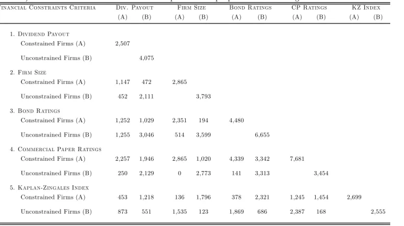
Table 1 reports the number of firm-years under each of the ten financial constraints categories
used in our analysis. According to the dividend payout scheme, for example, there are 2,507
finan-2 8Comprehensive coverage on bond ratings by COMPUSTAT only starts in the mid-1980s. 2 9
cially constrainedfirm-years and 4,075financially unconstrainedfirm-years. More interestingly, the table also displays the cross-correlation among the various classification schemes, illustrating the
differences in sampling across the different criteria. Of the 2,507firm-years considered constrained
according to dividends, 1,147 are also constrained according to size, while 452 are unconstrained.
Nearly half of the dividend-constrainedfirm-years are also constrained according to the bond rating
criterion, while the other half is unconstrained. Finally, note the remarkable discrepancy in
finan-cial constraint categorization provided by the KZ Index and all of the other measures, including
dividends. Only 18% (or 453) of the dividend-constrained firms are also constrained according to
the KZ Index, while about 23% of those firms are unconstrained according to the KZ Index.
B.3 Results
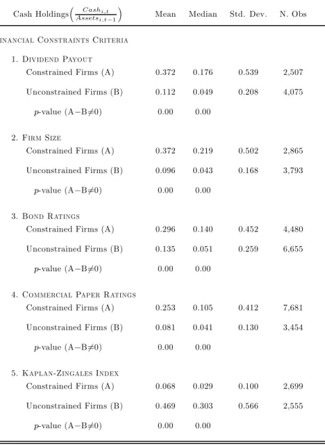
Table 2 presents summary statistics on the level of cash holdings of firms in our sample after
separating them into constrained and unconstrained categories. According to the dividend payout,
size, and the ratings criteria, unconstrainedfirms hold on average roughly 10% of their total assets
in the form of cash and marketable securities. This figure resembles that of Kim et al. (1998),
who report mean (median) holdings of 8.1% (4.7%). Constrained firms, on the other hand, hold
far more cash in their balance sheets; on average, some 30% of total assets. Mean and median tests reject equality in the level of cash holdings across groups in all cases. The one classification
scheme that yields figures substantially different from the others is the KZ Index, which tends to
classifyfirms that hold a lot cash as unconstrained. Notice that Kaplan and Zingales’ presumption
is that an unconstrained firm is one that has sufficient internal resources to fund its investments.
Our implementation of the KZ Index reflects their premises even though we have expunged cash holdings from their original empirical model.
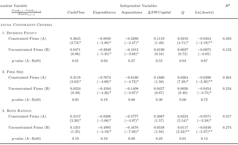
Table 3 presents the results obtained from the estimation of our baseline regression model
(Eq.(13)) within each of the above sample partitions. The model is estimated via OLS with firm
fixed-effects and the error structure (estimated via Hubber-White) allows for residual correlation within industry-years. In all cases the set of constrainedfirms display a statistically significant (at
better than 1% test level) positive sensitivity of cash to cashflow, while unconstrained firms show
insignificant cash sensitivities. The sensitivity estimates for constrainedfirms vary between 0.257
of additional cashflow (normalized by assets), a constrained firm will save around 1/3 of a dollar,
while an unconstrainedfirm does nothing. Notice that the difference in cashflow sensitivities across
constrained and unconstrainedfirms is statistically significant at the 5% level or better in all cases with only one exception (the KZ Index). These results are fully consistent with the prediction of our basic model.
TheQ-sensitivity of cash is always positive and significant for constrainedfirms, as predicted by our model. This sensitivity is sometimes also positive and significant in the unconstrained sample, but the magnitude of the coefficient is always larger in the constrained sample and the cross-group
differences are statistically significant at the 5% level in four of thefive cases. The coefficients on
the control variables also have the expected signs in our regressions. Investments, acquisitions, and size are negatively correlated with the change in cash. The coefficient on the change in net working capital is generally positive, but not always significant.
B.4 Robustness of the baseline results
We now subject our estimates to a number of robustness checks, in order to address potential concerns about model specification and other estimation issues. First, because of the possibility of outliers having undue influence on our results, we re-estimate our models using trimmed data
and (alternatively) via quantile regressions. Doing so does not materially affect our findings. In
addition we address the issue of coefficient stability over time by partitioning the data according to whether the observations come from the 1980’s or the 1990’s. Again, our results remain, although cross-sectional differences seem stronger in thefirst half of the sample.30
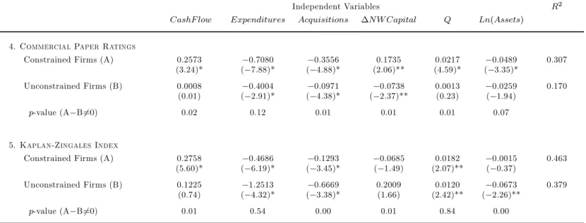
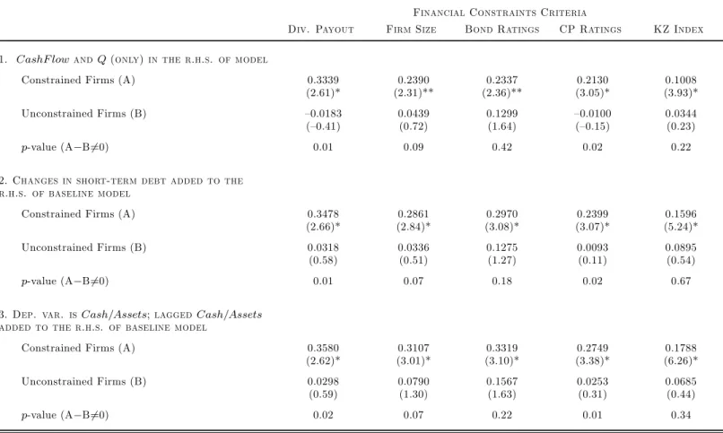
In addition, we present estimates of the cash flow sensitivity of cash using three alternative
empirical specifications in Table 4.31 At the top of the table (see first row) we report cash flow
sensitivities from a regression model that includes only the primitive elements of our basic theory
(CashFlow andQ) in the set of independent variables. The second specification we experiment with
adds changes in the ratio of short-term debt to total assets to the right-hand side of our baseline
model. We include this extra variable because of the possibility that firms use short-term debt to
build cash reserves. The third set of estimates in the table are from an alternative specification 3 0Tabulated results for the outlier-robust and subperiod regressions are omitted for brevity, but are available from
the authors upon request.
in which we move the lag level of cash/assets from the left-hand side to the right-hand side of our baseline model, effectively removing the constraint that lagged cash/assets should have a coefficient of 1. This last approach resembles more closely that in Opler et al. (1999).
In all, there are 15 pairs of constrained/unconstrained estimates in Table 4. In each case, the estimated cash flow sensitivity of cash for the constrained firms is higher (often by a factor of 2 or
more) than for comparable unconstrained firms. All of the constrained firm subsamples return a
statistically significant coefficient for cashflow, while none of the unconstrained cashflow estimates
are significant. The economic magnitude of the cash flow coefficient for the constrained firms is
reasonably consistent, varying from 0.21 to 0.35 in most specifications. Overall, Table 4 suggests that our results are robust to changes in model specification.
B.5 Dynamics of Liquidity Management: Responses to Macroeconomic Shocks A potential objection to the results presented above arises from the endogeneity of afirm’sfinancial
decisions. Since choice variables such as investment in net working capital and fixed assets enter
the baseline cash equation, it is possible that the levels of the estimates presented in Table 3 are
biased. Notice, though, that our main finding concerns therelative sizes of coefficients across two
subsamples of firms, and is not clear why any potential bias would occur differentially across the
two subsamples. In other words, any argument that endogeneity issues are responsible for our results has to explain both why our estimates of cashflow sensitivities of cash are positively biased,
and also why these biases are related to our partitions byfinancial constraints.
One way of providing independent confirmation of the interpretation we propose (as opposed
to the above “endogenous bias story”) comes from examining exogenous shocks affecting both
firms’ ability to generate cash flows as well as the shadow cost of new investment. Those shocks
should be economy-wide, simultaneously affecting all firms in the sample at a given point in time
and thus providing for cross-sectional contrasts. We find that examining the path of cash flow
sensitivity of cash holdings over the business cycle allows for an alternative test of the idea that financial constraints drive significant differences in corporate cash policies. To wit, if our conjecture
about those policies are correct, then we should see financially constrained firms saving an even
greater proportion of their cashflows during recessions. This should happen because these periods
compared to current investments as well as a decline in current income flows. The cash policy of financially unconstrained firms, on the other hand, should not display such pronounced patterns.
In other words, theresponses of cashflow sensitivity of cash to changes in aggregate demand should
be stronger forfinancially constrainedfirms. This should happen regardless of the levels of those
estimates, and the test thus sidesteps concerns with endogeneity biases in the baseline equation. To implement this test, we use a two-step approach similar to that used by Kashyap and Stein
(2000) and Campello (2002). The idea is to relate the sensitivity of cash to cashflow and aggregate
demand conditions by combining cross-sectional and times series regressions. The approach sacri-fices statistical efficiency, but reduces the likelihood of Type I inference errors; that is, it reduces
the odds of concluding that cash holdings respond to cashflow along the lines of out theory when
they really don’t.32
The first step of our procedure consists of estimating the baseline regression model (Eq. (13))
every year separately for groups of financially constrained and unconstrained firms. From each
sequence of cross-sectional regressions, we collect the coefficients returned for cash flow (i.e., α1)
and ‘stack’ them into the vector Ψt, which is then used as the dependent variable in the following
(second-stage) time series regression: Ψt=η+
2 X k=1
φkLog(GDP)t−k+ρT rend+ut. (15)
We are interested in the impact of aggregate demand, proxied by the real log of GDP, on the
sensitivity of cash to cash flow. The economic and the statistical significance of aggregate demand
can be gauged from the sum of the coefficients for the lags of GDP,Pφk, and from thet-statistics
of this sum. We allow for two lags of GDP to account for the fact that macroeconomic movements
spread out at different speeds throughout different sectors of the economy.33 A time trend (T rend)
is included to capture secular changes in cash policies. Finally, because movements in aggregate demand and other macroeconomic variables often coincide, in ‘multivariate’ versions of Eq. (15) we also include current inflation (log CPI) and interest rates (Fed funds rate) to ensure that ourfindings
are not driven by contemporaneous macroeconomic innovations affecting the cost of money.34
3 2
An alternative one-step specification – with Eq. (15) below nested in Eq. (13) – would impose a more constrained parametrization and have more power to reject the null hypothesis of cash policy irrelevance.
3 3Not allowing for lagged responses could bias our results if the distribution offinancially constrainedfirms happen
to be more concentrated in sectors of the economy that respond more rapidly to changes in demand. Our results are largely insensitive to sensible variations in the lag structure of Eq. (15).
3 4
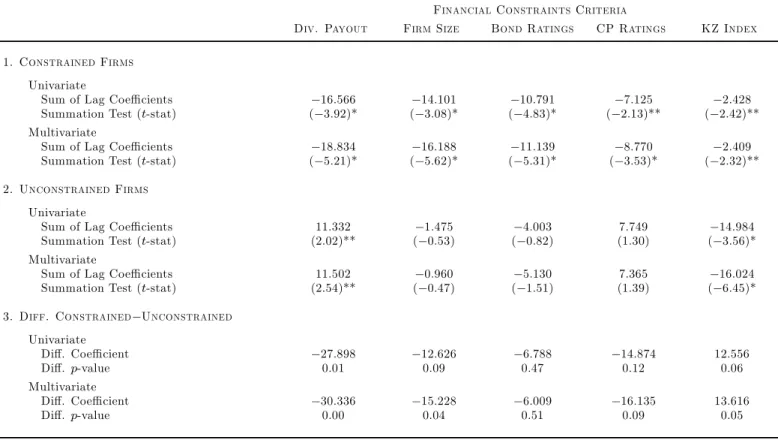
The results from the two-stage estimator are summarized in Table 5. The table reports the
sum of the coefficients for the two lags of GDP from Eq. (15), along with the t-statistics for the
sum. Panel A collects the results for financially constrained firms and Panel B reports results for
unconstrainedfirms. Additional tests for differences between coefficients across groups are reported
in the bottom of the table (Panel C). Standard errors for the “difference” coefficients are estimated
via a SUR system that combines the two constraint categories (p-values reported).
All of the GDP-response coefficients for the constrainedfirms displayed in Panel A are negative
and statistically significant at the 5% level or better, suggesting that constrainedfirms’ cash policies
respond to shocks affecting cashflows and the intertemporal attractiveness of investment along the
lines of our theory. In contrast, the response coefficients for the unconstrained firms presented in
Panel B display no clear patterns, but with only one exception (the KZ Index), are uniformlylower
than those of Panel A. The differences between those sets of coefficients in Panel C suggest that
the cashflow sensitivity of cash forfinancially constrained and unconstrainedfirms follow markedly
different paths over the business cycle. These differences are consistent with the ideas in the model of liquidity management we proposed above.
In order to gauge the economic significance of the estimates in Table 5, consider a scenario
in which the GDP falls by 1% over two years. Take two hypothetical firms, one constrained and
the other unconstrained according to size.35 Our multivariate regression estimates suggest that
while there is no effect on the propensity of the unconstrained firm to hoard cash, the cash flow
sensitivity of the constrained firm increases by around 0.15 over the two years. Given that the
overall propensity to save cashflows estimated in Table 3 is around 0.3, the effect of a recession on
the propensity to save appears to be substantial.
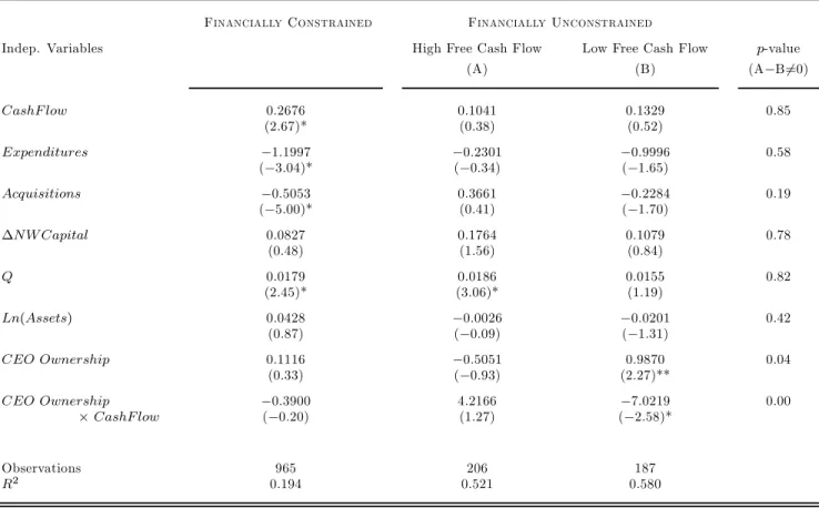
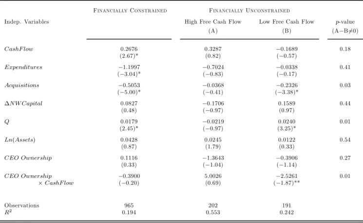
C
Agency Problems and Cash Holdings
Our model predicts that agency problems will lead otherwise unconstrained firms to display a
propensity to store greater portions of cashflows when management has poorly-aligned incentives.
This prediction holds only for thosefirms that become effectively constrained because of the desire
of managers to overinvest. If the unconstrained firm has sufficient financial slack so that it can
invest up to the manager’s preferred point, its cash policy will be observationally equivalent to those 3 5