Scalable Techniques for Trajectory Outlier Detection

(1)

A THESIS

SUBMITTED TO THE FACULTY OF THE GRADUATE SCHOOL OF THE UNIVERSITY OF MINNESOTA

BY

Usman Gohar

IN PARTIAL FULFILLMENT OF THE REQUIREMENTS FOR THE DEGREE OF

MASTER OF SCIENCE

Professor Eleazar Leal

(2)

c

(3)

Acknowledgements

Above all, I thank the Almighty for His Benevolence and for providing me with the strength and guidance to be where I am today.

I want to especially thank my advisor Dr. Eleazar Leal for his complete support throughout my research. He helped me whenever I came across difficulties in my research or writing and was always readily available. I thank him for guiding me through the process and keeping me on track.

I would also like to show my gratitude to Dr. Pete Willemsen, Director of Graduate Studies at the Department of Computer Science, University of Minnesota Duluth. His advising in the graduate seminar and otherwise played an important part in the successful completion of my thesis. I thank him for the opportunity and instilling in me the confidence to further pursue graduate studies.

Lastly, I want to acknowledge my family and friends for providing me with the moral support, encouragement and confidence throughout my research. This could not have been achieved without their support.

(4)

Dedication

First and foremost, this thesis is dedicated to my parents and my family, without whose constant support and encouragement, I would not have achieved this feat. They have provided me with unparalleled support and unconditional love.

To all my friends and colleagues, here at UMD and back home, who shared words of advice, encouragement and made up my social support. Lastly, a sincere dedication goes out to all the faculty members and staff at the Department of Computer Science who have been a constant part of my journey at UMD.

(5)

Abstract

The recent improvements in tracking devices and positioning satellites have led to an increased availability of spatial data describing the movement of objects such as vehicles, animals, etc. Such data is obtained by recording the positions of the objects at regular intervals and then arranging the collected positions of each object into a time-ordered sequence called trajectory. The high availability of trajectory data has permitted the execution of data analysis operations such as trajectory outlier detection, which consists in the identification of those trajectories that behave much differently from the rest of the trajectories in a database.

There are several time-critical applications such as traffic management systems, security surveillance systems and real-time stock monitoring, etc. which can be solved through trajectory outlier detection. However, the time-critical nature of such appli-cations imposes tight constraints on the execution time of trajectory outlier detection algorithms. To deal with these constraints, we propose three strategies to accelerate the performance of the existing trajectory outlier detection algorithm ODMTS. First, we consider using spatial data structures such as k-d trees and R-trees to improve the running time performance of the ODMTS algorithm for trajectory outlier detec-tion. Our results showed that by using R-trees we can improve the execution time of ODMTS by a factor of 10X. Our second strategy consists in harnessing the power of multiple CPUs to parallelize the ODMTS algorithm. This strategy yielded an exe-cution time improvement that scales linearly with the number of cores, which in our case achieved 32X. The third strategy consists in a new partitioning-based streaming algorithm, called PDMTS, that leverages data streams in order to find trajectory outliers. Our experiments on real-life datasets showed that our proposed algorithm detected 45% outliers more than ODMTS but is 18% slower due to partitioning.

(6)

List of Tables

4.1 Summary of Experimental Datasets . . . 29

4.2 Summary of Experimental Datasets . . . 37

(10)

List of Figures

1.1 This figure illustrates outliers in a time-series . . . 1

2.1 A sample trajectory. . . 6

2.2 Trajectory Segmentation . . . 7

2.3 An example to illustrate outliers in a 2-D Dataset . . . 8

2.4 Example of candidate trajectories in a Window . . . 16

2.5 Detecting Outliers in the example in 2.4 . . . 17

2.6 Example to describe the distance measures . . . 18

3.1 This figure illustrates the use of the Haversine Approximation between two geo-coordinate points . . . 22

4.1 An example of inconsistent sampling rate . . . 30

4.2 Varying number of cores (15 min window) . . . 31

4.5 Varying number of cores . . . 33

4.6 KD-Tree vs R-Tree Comparison (T-Drive) . . . 34

4.7 KD-Tree vs R-Tree Comparison (Geolife) . . . 35

(11)

4.9 ODMTS Performance . . . 39

4.10 ODMTS Performance . . . 40

4.11 Overall Performance Comparison between ODMTS and TRAOD (Italy Power) . . . 41

4.12 Overall Performance Comparison between ODMTS and TRAOD (Earth-quake) . . . 42

(12)

1 Introduction

The ubiquitous use of location-based devices such as smartphones and GPS has led to the availability of massive amounts of location data worldwide. These data can be used to track the movements of objects such as vehicles, animals, goods and weather patterns etc. by forming trajectories, which consist of time-ordered geo-coordinate data points that describe the movement of an object. The availability of such data makes it possible to execute various data analysis operations such as trajectory outlier detection. Trajectory Outlier detection aims to search for anomalies in data that do not conform to the expected behavior. Figure1.1 shows two outliers in a trajectory. It can be observed how the two peaks in red behave differently as compared to the majority of the data points.

(13)

1.1 Challenges of Trajectory Outlier Detection

The challenges of outlier detection are:

1. Scalability:

When finding trajectory outliers, one is dealing with a Big Data problem. The reason for this is that trajectory outliers are searched for in databases with many trajectories. Moreover, each trajectory consists of many points, each of which can have many dimensions. In addition to this, trajectory similarity measures to compare the similarity of two trajectories with n points each usually have a worst-case time complexity of O(n2_{), which means that finding trajectory}

outliers is a very time-consuming operation. 2. Inconsistent samping rates:

Another challenge that comes up very often is the inconsistent sampling rates. This refers to the fact that the datasets have gaps in the records between them due to inconsistent recording of the position of the object e.g. this could be due to unavailability of connectivity in some areas or that the sampling rate is too low to collect enough data points to make an accurate decision about the trajectory. This affects outlier detection techniques because absence of up-to-date information across multiple trajectories at a certain point in time can lead to incorrect classifications.

3. Similar behavior:

The characteristics of trajectories are usually very similar across time. There is little to no sudden changes in the behavior of the data points compared to other data streams. This makes it harder to detect outliers because they are hidden among normal trajectories due to resembling characteristics.

(14)

1.2 Applications of Trajectory Outlier Detection

Real-time detection of trajectory outliers play an important role in making key decisions in various applications because these anomalies can have a critical and significant impact. For example, in 2016, alcohol-impaired crashes accounted for 28% of all crash fatalities in the United States [1]. Abnormal driving characteristics such as changing lanes frequently, can be termed as outliers in traffic management systems [2]. Detecting such outliers in traffic management systems can potentially flag drunk driving and speeding, etc. which can help reduce fatal crashes. Similarly, outlier detection in trajectories can be extended to financial markets. In May 2010, one such anomaly caused a market crash that resulted in a huge economic loss in the figure of billions of dollars [4]. By modeling price, volume and other parameters of stocks at a given time as a trajectory stream, it could be possible to prevent such negative events in the future. We could also identify stocks that have the potential to perform better and increase dividends. Another important application is related to security surveillance [26]. In a military situation, the commander must be aware of all movements of his group. If some members of the group do not operate together, they will be classified as outliers. This can help organize the group in a manner that ensures protection and reduces risk. Hence, detection of outliers in real time can positively impact decisions in various applications.

1.3 Contribution

The contribution of this thesis consists in addressing the scalability issue of tra-jectory outlier detection. To this end, we propose three strategies to improve the running performance of the existing ODMTS algorithm [26] in this thesis.

(15)

Our first strategy consists in using spatial data structures such as k-d trees [1] and R-trees [7] to improve the running time performance of the ODMTS algorithm for trajectory outlier detection. In our initial experiments and code profiling, we observed that the slowest factor in the ODMTS algorithm was the range query search. To address this, we decided to use data structures that could help reduce the time of the range query search.The motivation behind using k-d trees and r-trees was the characteristic of these data structures to store k-dimensional points at each node, as is in the case of trajectories.

Our second strategy consists in harnessing the power of multiple CPUs to par-allelize the ODMTS algorithm. As discussed above, the range query search was the slowest block in the ODMTS algorithm. To improve execution time, we explore the possibility of dividing the workload of the range query search among multiple cores and and explore the scalability of the algorithm.

The third strategy consists in proposing a new partitioning-based streaming algo-rithm, called PDMTS, for trajectory outlier detection that leverages data streams in order to find trajectory outliers. The key-idea here is that some outliers are hidden as sub-trajectories in trajectories, that are not otherwise picked up by outlier detection techniques such as ODMTS. This strategy uses the partitioning technique in [13] and then detects outliers by comparing the spatio-temporal characteristics across other trajectories.

1.4 Organization

The rest of this thesis is organized as follows. Chapter2 presents the background of our work, including related work. Chapter3 presents the details of the implemen-tation of our work. Chapter 4 presents our experimental results and observations.

(16)

(17)

2 Background

2.1 Trajectory

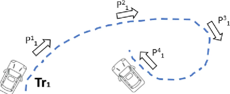
A single multidimensional point P_ij generated from a moving object O, using a tracking device, at time-bintj, is called a trajectory point of the trajectory Tri. The

trajectory of a moving object O is then defined as a sequence of such trajectory points produced at time-bins {t1, t2tj} denoted as T ri = {Pi1, Pi2, ...P

j

i} as shown below.

A time-bin is the most smallest unit of time interval for a trajectory. Informally, a trajectory can be defined as the path that an object follows in time

Each point P_ij corresponds to the location of an object at the time-bin ti, with

coordinates (xi, yi). . Figure2.1 shows an example of a trajectory of a vehicle.

(18)

2.1.1 Length of a Trajectory

The length Len of a trajectory is the number of data points or multidimensional

points in the path that the object has followed in time. The length of the trajectory in Figure 2.1 is four.

2.1.2 Trajectory Segmentation

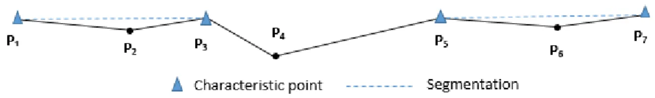
An important aspect of trajectory analysis is segmentation where the original tra-jectory is broken down into multiple line segments based on a characteristic. Leeet al. [14] segment trajectories on characteristic points which are points on the trajectory where the trajectory changes direction rapidly. This threshold has been predeter-mined for the dataset used in the work. Figure2.2illustrates trajectory segmentation. In the segmented trajectory, the property or the characteristic stays constant. This is helpful in [18] where the a certain activity of a birds is being analyzed, such as soaring etc. This can also be used to segment images with similar texture or patterns as in [11]

2.1.3 Trajectory Streams

A data stream is called a trajectory stream if the points that makes up the stream are gps points taken from a moving object sampled at a regular interval [12]. This can be achieved using a GPS sensor.

(19)

2.2 Outlier

Outliers are patterns in data that do not conform to a well defined notion of normal behavior [3]. An outlier has also been described as a data object that is grossly different from or inconsistent with the remaining set of data [8]. We explain the concept with the aid of figure 2.3. The three grouped data points C1, C2, C3 are

”normal” because they exhibit similar behavior and are in close proximity, which is also one of the parameters to determine whether a data point is an anomaly. Since the rest of the points outside these regions are significantly further away, all these points are considered outliers.

Figure 2.3: An example to illustrate outliers in a 2-D Dataset

Outliers can be present in a dataset due to a number of factors but not limited to inconsistent sampling, malfunction or some malicious activity depending upon the application [3].

(20)

2.2.1 Types of Outliers

There are essentially three different types of outliers [3]. The type of outlier algorithm to be used is linked with what type of outliers we are hoping to catch. The outliers are classified as follows:

Point Outliers

A data point is classified as a point outlier if the point on it’s own is significantly different from the rest of the points in the data set. Going back to figure2.3, all of the individual points outside the three normal regions (C1, C2, C3) are all point outliers.

Most application of point based outliers are one dimensional data points such as price of stock, credit card fraud etc. In the case of stocks, if the price of a particular stock is relatively higher than the rest of the stocks in the same category, it will be considered an outlier in that context.

Contextual Outliers

Contextual Outliers, or conditional outliers, are data points that are considered outliers only in a specific situation but not otherwise. The context usually needs to be pre-defined and is derived from the dataset based on it’s properties. There are mainly two categories of attributes used to determine the outlier:

1) Contextual:

These attributes help restrict the environment of the data points, or in other words, provide the context. In our work, these contextual attributes are the geo-coordinates i.e the latitude and longitudes of each data points. Another example of such attributes is time which helps us restrict the data point to a position in time.

(21)

Both of these attributes are an integral part of our work.

2) Behavioral:

These attributes are more related to the properties of the dataset. For instance, the average power consumed, average prices of stock etc.

Both of these attributes are used together detect outliers. The values of the behavioral features of the data instances are checked within a specific context using the contextual attributes to determine whether their behavior warrants to term it as an outlier or not.

One example of a time series data where contextual outliers are found is credit card fraud detection. In this case, statement balance can be considered as a behavioral attribute while the time of purchase can be considered a contextual attribute. During a normal year, a person is expected to have higher balances around the new year while the rest is on average similar. If for a particular normal month with no event, for instance March, a person has a balance of $1000 while the average balance for this month is a $100 otherwise, this indicates that the behavior of the data instance is not normal. Hence, this should be classified as an outlier.

However, this also makes the outlier detection problem more complex due to the added condition of the context. For example, during summers the buses take a normal route to school but take a detour during snowy days. Without context, that would be recognized as an outlier but not in this case.

In [24], the authors aim to detect outliers in precipitation data. The contextual attributes used here are both time and location. So if in a particular month, the average precipitation is significantly higher than normal, the data points are termed outliers.

(22)

that can affect whether you can use it or not.

Collective Outliers

These outliers are the exact opposite of point based outliers. When a group of data instances is significantly different to the rest of the dataset, then they are termed as collective outliers. In other words, the data points on their own are not outliers until they are part of greater subset of the dataset.

These types of outliers only exist in datasets where the data instances are somehow related to each other in sequence. Some of the work in this area has been conducted for spatial data in [20].

Detection of collective outliers makes the outlier detection problem even more challenging because finding sub-sequences of the trajectory streams makes the classi-fication even more complex.

2.3 Related Work

Many studies have been undertaken to develop algorithms to detect trajectory outliers. These algorithms are categorized as follows: Outlier Detection in Static Datasets and Outlier Detection in Data Streams. These can be further classified in distance-based and density-based approaches. In this work, we will cover Outlier Detection in Static Datasets and Data Streams.

2.3.1 Trajectory Outlier Detection in Static Datasets

One of the first work on trajectory outlier detection used distance-based metrics for their approach [10]. They proposed deriving various features from the trajectories

(23)

trajectory is an outlier [10] Since this exercise is conducted only once, is not applicable to a data stream. This means that the feature set will not stay relevant and fresh compared to the current time.

In [15], the author proposes a new approach to address outlier detection. The approach involves identifying discrete patterns in trajectories called motifs which are used to extract and create a feature set. A rule-based classifier is then used to classify these trajectories based on the feature set into outlier or normal. Since this algorithm has a training stage based on these motifs, it requires labeled data that is not available in our data streaming environment as the outlier detection is real-time.

For the detection of fraudulent taxi driving patterns, Zhang et al [29] proposed the use of historical trajectory data sequences. The method involves grouping trajectories that have the same pick up and drop-off points and then finding all the trajectories that do not follow these paths for the same starting and end points.A similar ap-proach is used in [4] to discover dubious taxi driving, however, it is detected after the destination is reached which does not apply in our case where we need to detect outliers in a streaming fashion.

Another proposal by Lee et al. [13] involves two steps where the trajectories are first divided into partitions called sub-trajectories. In the second step, distance-based feature sets are created which are used to detect outliers. This approach only detects outliers within trajectories, not in the whole data stream. In our work, we actually modify this algorithm (TRAOD) so it can be used for Data Streams and not just within a single sub-trajectory.

(24)

2.3.2 Outlier Detection in Trajectory Data Streams

In [2], the authors use the idea of historical trajectory segments of one very long particular and continuous trajectory. It is assumed that the characteristics or the behavior of the trajectory does not change in a very small period of time. The method proposes using windowing to form trajectory segments and then comparing the segments to each other to determine whether they are outliers or not. This goes against our objectives of detecting outliers in a group of other trajectories in close proximity in time and space.

Another work that is very closely related to our objectives, is the TOP-EYE trajectory outlier detection [5]. The authors propose using a evolving method that involves computing a score that evolves over time and which determines whether the trajectory is an outlier at any given time. This method also includes a decay function that reduces the effects of the previous trajectories on the score so as to keep it fresh. However, this method applies a grid which means only trajectories passing through the grid are considered as part of the score.

Liu et al. [16]focused on discovering relationships and causal interactions between outliers in traffic data. In this work, the propose the construction of outlier causality trees based on spatio-temporal characteristics. First, the city is divided in regions and then vertex constructed accordingly. However, this work is not related to detect-ing trajectory outliers in movdetect-ing objects, rather investigatdetect-ing the any relationships between any historical traffic outliers.

(25)

2.3.3 Outlier Detection over Massive-Scale Trajectory Streams

(ODMTS)

Trajectory

As discussed earlier, a trajectory of a moving object O, is defined as a sequence of trajectory points produced at time-bins t1, t2tj denoted as T ri={Pi1, Pi2, ...P

j i}.

TimeBins

Timebins refer to the smallest time unit for the recorded location of a point. Using our earlier definition of trajectories, pj₁ corresponds to the point at timebins j. This does not have to refer to a point at a particular location in time rather any event along time.

Windowing

This work also utilizes the concept of periodic windowing [6]. For every experi-ment, a window size W and slide size S are specified. This restricts the number of trajectories as only the trajectories or data points whose respective timebins fall in that window are considered for the experiments. After the ending time of the win-dow is reached, the winwin-dow slides byS to the right. There is no overlap between the windows to avoid any repetition of data points in the windows.

Distance Function

To determine the closeness of two trajectories, or in other words the proximity, we simply use the Euclidean Distance. This is incorporated in the function dist(pj_i, pj_k) from here onwards. This function gives us the Euclidean distance between two points

(26)

of a trajectory in timebin Tj. We use Euclidean distance for sake of simplicity but other distances measures can also be used here as in TROAD [13]

Point Neighbor

If two trajectory points, pi_j, pi_k, in the same timebin Ti are within a distance of d

of each other, where d is a distance threshold, then those two points are considered point neighbors of each other. In other words, if for these two points dist(pi

j, pik) ≤

d, the points are point neighbors [26].

Trajectory Neighbor

The paper then extends the definition of point neighbors to define Trajectory Neighbors. In a particular window Wc, a trajectory is called a neighbor trajectory

only and only if for at least thr timebins the trajectories share point neighbors in each of these timebins. In terms of the notation, for trajectory T ri and T rj, if in at

least thr timebins, pi is a point neighbor of pj in all of these timebins, then the two

trajctories are denoted as neighbors of each other [26].

Trajectory Outlier

Using the above two definitions, a Trajectory T ri is considered an outlier in

win-dow Wc, if in at leastthr timebins, there are less k number of points that are point

neighbors, where k is the neighbor count threshold.

Formally, for a Trajectory T ri, distance threshold d, neighbor threshold k and

timebin count threshold thri, it is considered an outlier if it has fewer than K

trajec-tory neighbors [26].

(27)

words, other trajectories need to be behaving very similarly and consistently for it to be classified as an inlier in the particular window.

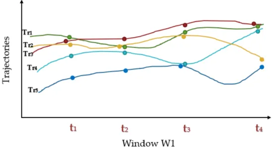
Figure 2.4: Example of candidate trajectories in a Window

Let’s take a look at the example in figure 2.4 to better understand this. In this specific window, we have a total of 5 trajectories, namely T r1toT r5 that have been

sampled across 4 timebins t1tot4. In Figure 2.5, we describe how the algorithm works

over the 4 timebins in the window. T ri.N T will store the information for trajectories that share at least one point neighbor with Tri whereasT ri.T List will stores the ID’s of the corresponding neighboring timebins.

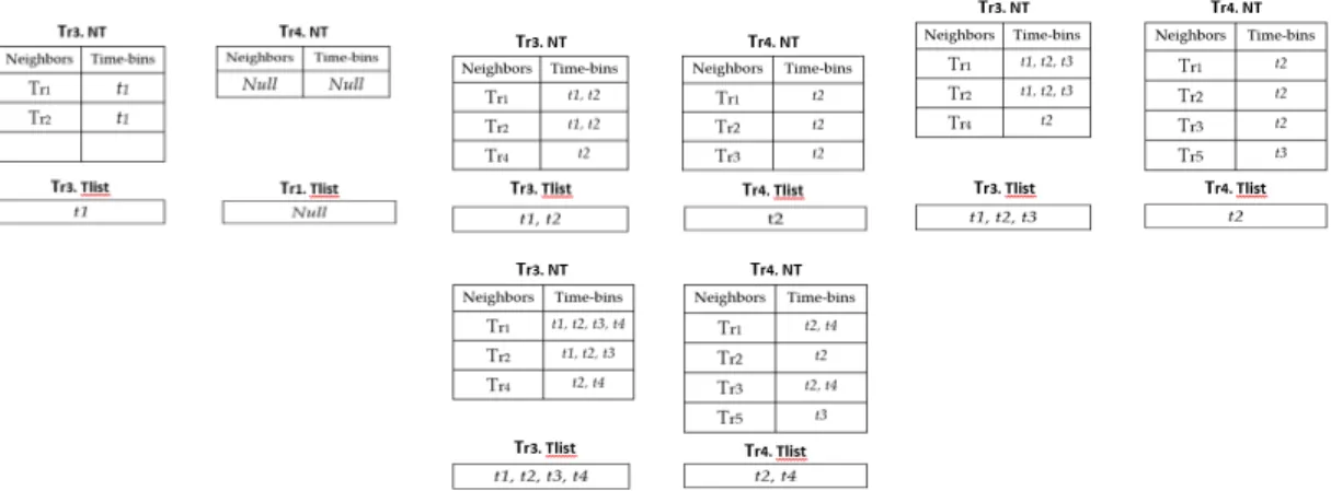
For this example, let’s have T hr = 2 and K = 3 and we will just look at the Trajectories T r3 and T r4. The In the first timebin t1, T r3 has Tr1 and Tr2 as its point neighbors as reflected in T r3.N T. Since the number of point neighbors for one timebin is greater than then threshold Thr, t1 is also listed in the T r3.T list table. The same process is followed for T r4 and again across all the timebins until the end of the window is reached. The final table in2.5 demonstrates what the table will look

(28)

Figure 2.5: Detecting Outliers in the example in 2.4

like after the algorithm finishes processing. To classify a trajectory as inlier, it must have atleast K entries in the T ri.T listtable. In this case, K = 3 and onlyT r3.T list

fulfills this criteria. Hence, T r4 is classified as an outlier.

When the algorithm reaches the end of the window, it moves to the right by the window size without any overlap and the process is repeated.

2.3.4 Trajectory Outlier Detection (TRAOD)

In the earlier subsection, we discussed this algorithm briefly. Here we will talk about the algorithm in a bit more detail. The main idea of the algorithm is to detect the hidden sub-trajectory outliers within a single trajectory by partitioning the trajectory and then determining whether they qualify as outliers based on distance based measures. The algorithm has two main phases: partitioning and detection phase [13].

Partitioning

The authors start off with a very basic idea of partitioning to ensure high quality i.e. to extract all possible partitions. The propose partitioning each trajectory at

(29)

it’s base unit, which they describe as the smallest unit of a trajectory according to the data type [13]. In our case, this turns out to be sampling of the location and time of the trajectory. Hence, the base unit can be every single point but can include multiple points if the total sampling is less than the interval of interest.

Once the partitions have been made according to the base units, it is extended by fine tuning them only for those partitions that are likely to be outlying. The initial partitioning is done to achieve preciseness and conciseness which is achieved by using the MDL Principle. We will not go into too much detail since we have not made major changes to this phase.

Detection Phase

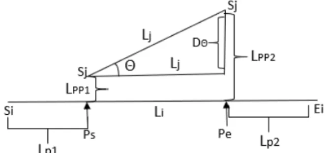
This work also proposes using distance measures to determine whether each tra-jectory segment is an outlier. But rather than simply using Euclidean Distance as in [26], the authors have proposed a distance function composed of three different types of distance measures: parallel distance (Dp), perpendicular distance (Dpp) and angle

distance (Da).

Figure 2.6: Example to describe the distance measures

The figure 2.6 has been adapted from [13]. The figure shows two lines Li and Lj

and the distance measures that the algorithm calculates. The distance equations are as follows:

(30)

P erpendicular(Dpp) = Lpp21+Lpp22 Lpp1+Lpp2 (2.1) P arallel(Dp) =M IN(Lp1, Lp2) (2.2) Angle(Da) =Lj ×sinθ (2.3)

These three components are merged together to form a distance functiondist(Li, Lj)

that incorporates weights.

dist(Li, Lj) =w0·Dpp+w1·Dp+w2·Da (2.4)

Hence, if the distance, using the distance function, between two partitions is greater than a threshold, the trajectory is classified as an outlier.

(31)

3 Implementation

The goal of the thesis work can be summarized as follows:

• Explore the possibility of improving running performance of outlier detection algorithm using spatial data structures.

• Improving the running performance of ODTMS algorithm by harnessing the power of multiple CPUs to parallelize the ODMTS algorithm.

• Introducing a new partitioning-based streaming algorithm, called PDMTS, for trajectory outlier detection that leverages data streams in order to find trajec-tory outliers.

In this section, we discuss the details of the implementation of our work. Section

3.1 presents the implementation of spatial data structures to improve the running performance of ODMTS. Section 3.2 presents the parallelized ODMTS algorithm to harness the power of multiple CPUs. Finally, in section 3.3, we discuss the details of PDMTS.

3.1 Serial Implementation

As discussed in the section 2, the ODMTS algorithm primarily uses the distance between trajectories to determine whether they are close enough to be neighbors. However, trajectories are a sequence of geo-coordinate points where each point cor-responds to the location of an object in time. Before we can calculate the distance

(32)

between two trajectories, we need to convert the coordinates to a metric unit. This is because the ODMTS algorithm requires the metric distance between two trajectories to test its outlying behavior, not simply the latitudes and longitudes. To this end, we use the Haversine approximation.

3.1.1 Haversine Approximation

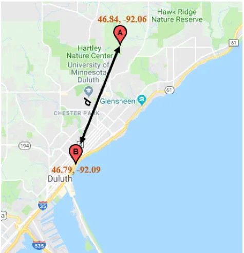
The Haversine Formula calculates the shortest distance between two points on a sphere given their latitude and longitudes [23]. In other words, it calculates the bird eye distance between two points on a sphere. Figure 3.1 illustrates how to computer the straight-line distance d between two markers A and B.

a= sin2(∆φ 2 ) +sin 2₍∆γ 2 )×cos(φ1)×cos(φ2) c= 2×(√a,√1−a) d=R×c where: φ is the latitude γ is the longitude

R is the radius of the Earth

The Haversine formula returns the distance between two geo-coordinate points in metres, which is directly injected into the algorithm.

3.1.2 Bottleneck/Optimization

(33)

bot-Figure 3.1: This figure illustrates the use of the Haversine Approximation between two geo-coordinate points

execution of the algorithm. We profiled our code to determine the execution time for each block of code. To this end, we used Python’s cProfile module [19] to determine various profiling parameters including total execution time. Our profiling revealed that the spatial search block of Algorithm1, which corresponds to (lines 1-3) on page 22, took the most time. This is due to the exhaustive nature of the search. The profiling for the algorithm is included in Chapter 4.

We looked into two different spatial data structures to optimize the ODMTS algorithm and compared their performances in solving the nearest neighbor problem when it comes to outlier detection; namely k-d trees and R-trees. A k-d tree is a

(34)

data structure that uses associative searches to retrieve stored information [1]. We used the Nearest neighbor search within a Radius R to find all the neighbors of a trajectory in the k-d tree. The k-d tree stores records in the form of k-dimensional points where the nodes represent separating planes. To implement the tree structure, we used the Python Numpy and Scipy libraries. The average runtime for a k-d tree isO(nlogn). An R-tree, on the other hand, can store rectangles and bounding boxes as opposed to point vectors [7]. R-trees are also balanced trees so the data can be changed without having to rebuilt the whole tree. The execution time for both the data structures is evaluated in Chapter 4

Algorithm 1 Distance Based Outlier Detection (ODMTS) Input Set of Trajectories, parameters: d,k, thri

Output Trajectory Outliers 1: for each T Ri do 2: for each T Rk do 3: if dist(pj_i, pj_k)< d then 4: T Ri.N T.insert(T Rk) 5: end if 6: end for

7: if T Ri.Count(tbin) >thr then

8: T Ri.T list.insert(tbin)

9: end if 10: if T Ri.size < k then 11: T Ri is an Outlier 12: end if 13: end for

3.2 Parallel Implementation

The second part of our work evaluates exploring whether the algorithm scales when implemented across multiple cores and the trade-off between increased effi-ciency and increased memory usage. To improve the running time of the algorithm,

(35)

we implemented it in parallel on multiple cores using both k-d trees and R-trees using the multiprocessing module of python [17]. Python has two different parallel implementations. The threading module which creates separate threads and uses a lock to prevent race conditions. Due to this, multiple threads will not be able to access the same tree to get the results for the range query. On the other hand, the multiprocessing module spawns new processes that have a slight overhead, however, it does not block other processes from accessing the same tree at the same time, pre-venting race conditions. In our case, we prefer the use of spawning new process due to high frequency of tree accesses. The parallel algorithm is shown in 2. results for the parallel implementation are discussed in Chapter4.

Algorithm 2 Parallel - Distance Based Outlier Detection (ODMTS) Input Set of Trajectories, parameters: d,k, thri

Output Trajectory Outliers

1: Insert all trajectory points in K-D/R Tree 2: Divide the Trajectory Dataset into Count(cores) 3: Insert divided Datasets in separate T RiList

4: for each core do

5: Run a Ball-Point Query Search on all Trajectories in T RiList

6: Insert query search result in N eighboriList

7: for each in N eighboriListdo

8: if Count(N eighboriList[T Ri]) <k then

9: T Ri is an Outlier

10: end if 11: end for 12: end for

3.3 PDMTS

In the final part of our work, we introduce a modified version of TRAOD [13] called Partion based Outlier Detection over Massive Trajectory Streams (PDMTS). The original algorithm, as discussed in 3, does not apply to real-time streaming

(36)

trajectory data. It works in an offline mode where all outliers are detected from a dataset that has been recorded earlier. Furthermore, as discussed earlier, this method only applies to finding outlier sub-trajectories in the same single trajectory, instead as part of many trajectories. This means the inspiration and applications of our work do not apply to this algorithm. We tweak the algorithm by including the concept of windowing and temporal comparisons to enable it to be deployed for real-time detection.

As discussed in Chapter 2, the original algorithm first partitions the trajectory into sub-trajectories and then calculates three different distances (parallel, perpendicular and angular). It uses a distance formula that combines these three distances to return a single value distance between two partitions. If the value returned is greater than a threshold, that is predetermined according to the dataset, the sub-tracjectory within that of the particular trajectory is deemed as an outlier.

The issue here is that this method does not apply to retime streaming online al-gorithm. To achieve this, we introduce the concept of temporal comparisons from the Distace-Based Outlier Detection algorithm [26]. Instead of comparing the partitions only with other partitions from the current trajectory, we compare the partitions to the all other partitions of all the trajectories within the specific window. The algorithm is illustrated in 3 below.

As seen in algorithm 3, this algorithm follows the same idea of partitioning as in TRAOD. Where it differs is, the Outlier Detection phase. Here we incorporate the same parameters as the Distance-Based outlier algorithm i.e distance threshold d, neighbor threshold k and timebin count thresholdthri. If the number of neighbor

(37)

Algorithm 3 PDMTS

Input Set of Trajectories, parameters: d,k, thri

Output Trajectory Outliers 1: —* Partioning Phase *— 2: for each T Ri do

3: Partition T Ri at coarse granularity using MDL (Li)

4: end for

5: —* Detection Phase *— 6: for each partition Li do

7: for each partitionLj do

8: if dist(pj_i, pj_k)< d then 9: T Ri.N T.insert(T Rk)

10: end if 11: end for

12: if T Ri.Count(tbin) >thr then

13: T Ri.T list.insert(tbin)

14: end if

15: if T Ri.size < k then

16: T Ri is an Outlier

17: end if 18: end for

(38)

4 Results

This chapter is divided in two separate sections; Outlier Detection using Multi-Cores and S-TRAOD. In the first section, we will discuss the results of optimizing the Outlier Detection Algorithm (ODMTS) using K-D/R tree and multiple cores. The second section will discuss the results of the comparisons between ODMTS and the streaming algorithm we propose. The overall structure for each section will be as follows; experimental setup i.e. both the hardware and software specifica-tions, datasets performance measures and the results and observations

4.1 Outlier Detection in Static Data Using

Multi-Cores

4.1.1 Experimental Setup

Hardware

All the experiments have been performed on Akka, the UMD server machine, which has a total of 40 cores with hyper-threading, 512 GB RAM and is running Ubuntu 16.04.5.

(39)

Software

The algorithm and the parallel component have been implemented on Python 3.7. Python provides the multiprocessing library [17] that supports spawning multiple processes to make use of the multiple processors on a machine.

Multiprocessing Package

This package provides the API to take advantage of multiple processes on a com-puter. The package does not use the Global Interpreter Lock, unlike the threading module, and the GIL prevents a race condition since the threads share the same mem-ory. Hence, threads cannot run concurrently with the GIL. On the other hand, the drawback of spawning new processes is that each process has a separate memory space and cannot share objects between each other as easily. Secondly, spawning new pro-cesses introduces latency. However, our parallel implementation does not require any memory sharing and the performance gain from using multiple CPUs overshadows the latency incurred.

4.1.2 Datasets

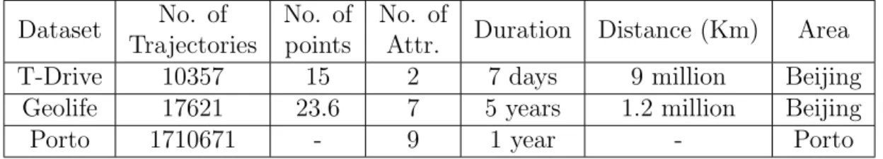
To evaluate the results of the parallel implementation, we need a big dataset to test the limits of memory usage and impact of increasing the number of cores. For those experiments we used two real datasets, T-Drive and Geolife. Table 4.1 gives a summary of the datasets used in the experiments . The T-Drive trajectory dataset is real GPS trajectory data that contains one-week trajectories of 10,357 Taxis in Beijing from Feb. 2 to Feb 8, 2008 [27][28]. This dataset has a total of 15 million points and the trajectories cover a distance of about 9 million kilometers. The dataset has inconsistent data sampling and the average sampling interval is approximately

(40)

Dataset No. of Trajectories

No. of points

No. of

Attr. Duration Distance (Km) Area

T-Drive 10357 15 2 7 days 9 million Beijing

Geolife 17621 23.6 7 5 years 1.2 million Beijing

Porto 1710671 - 9 1 year - Porto

Table 4.1: Summary of Experimental Datasets

177 seconds and the average distance between two time-consecutive points in each trajectory is 623 meters [27][28]. The format of the dataset is as follows:

5, 2008-02-06 14:25:09, 116.57115, 39.8564

Where the comma separated values delineateTaxi ID,Date Time,Longitudeand Latitude respectively.

The Geolife real life trajectory dataset was collected as a part of Microsoft Re-search Asia project which involved around 182 participants that recorded their move-ments over a period of five years from April 2007 to August 2012 [31][30][25]. This dataset contains a total of 17,621 trajectories that cover a total distance of 1,292,951 kilometers and a time duration of 50,176 hours. [4] This dataset is generated by different outdoor activities from jogging, driving, cycling to taking the bus home. This dataset also has variable data sampling rates, however, the majority of them are sampled 1-5 seconds. The format of the dataset is as follows:

39.8564, 116.57115, 0, 492, 40097.5861, 2009-10-11, 14:04:03

Where the comma separated values delineate Latitude, Longitude, Set to 0, Al-titude, Date (no. of days), Date and Time respectively.

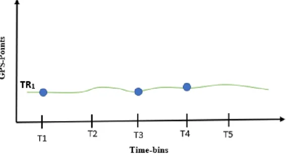
Time granularity of 1 min were used to model the time-bins. As the algorithm depends on the spatial and temporal characteristics, it is important to address the

(41)

nearest two-time bins and using them to extrapolate the approximate value of the trajectory point. For example, in the diagram below4.1, points are missing for time-bins T2 and T5. To calculate T2, we take the average increase of T1 and T3, the two closest time-bins and use it to approximate the value. The same goes for T5, however, T4 and T3 are used instead. The experiments were run for 15 min, 30 min and 45 min windows to compare the execution times for the algorithm in parallel.

Figure 4.1: An example of inconsistent sampling rate

4.1.3 Performance Measures

We evaluate the performance of the multiple cores by measuring the total program execution time. The total program execution time is calculated from the time when the process is first spawned to the time it terminates. Firstly, we keep the threshold thr constant and increase the number of cores from 1 to 32, incrementing each time by a power of 2. The experiments are repeated for a window size of 15,30 and 45

(42)

mins respectively. Secondly, we repeat the experiments and measure the Memory Consumption when we increase the number of cores.

4.1.4 Results and Observations

Impact of the number of cores on Execution Time

In this section, we evaluate the impact of the number of cores on execution time. For this experiment, the window size is varied from 15 mins to 45 mins in a 15-min increment. This is to evaluate whether the algorithm scales if the number of points in the window is increased. The threshold thr is kept constant.

(a) T-Drive _{(b) Geolife} (c) Porto

Figure 4.2: Varying number of cores (15 min window)

Figure4.2demonstrates the impact of the number of cores on execution time using the two datasets. The time in seconds is indicated on the y-axis whereas the x-axis is the number of cores. The y-axis represents the average execution time for N number of cores working concurrently. As can be seen from both Figure 1 (a) and (b), as the number of cores is increased by a power of 2, the average execution time decreases almost by half each time. Both graphs exhibit this behavior as can be seen from the decreasing curve of the bar plots. The execution time decreases since the workload is

(43)

execution time every time the number of cores is doubled. The red error bars denote the standard deviation and have been enhanced in size to make them visible since the standard deviation for the experiments was very low.

(a) T-Drive (b) Geolife (c) Porto

Figure 4.3: Varying number of cores (30 min window)

Our experiments have suggested that the number of points processed by each core did not have a significant impact on the scaling of the algorithm. The number of points increased from almost 40 million to 125 million. However, the algorithm still scales i.e. each time the number of cores is increased by a factor of 2, the execution time is halved, as seen from figures 4.2,4.3 and 4.4. Additionally, it can be seen that the execution time has increased for corresponding number of cores in figures4.2,4.3

and 4.4 when the window size is increased, which can be explained by the increased number of points the cores had to process. However, the results in figures 4.3 and

4.4 are very similar to figure 4.2. The bar plots show the same behavior as figure

4.2 where increasing the number of cores halves the execution time and scales as expected.

(44)

(a) T-Drive (b) Geolife (c) Porto Figure 4.4: Varying number of cores (45 min window) Impact of the number of Cores on Total Memory Consumption

In this experiment, we evaluate the impact of increasing the number of cores on the total memory consumption. The window size (15 mins) and the threshold thr is kept constant.

(a) T-Drive (b) Geolife (c) Porto

Figure 4.5: Varying number of cores

Figure 4.5 demonstrates the effect of increasing the number of cores on the total memory consumption. The total memory consumption in MB is given on the y-axis and x-y-axis denotes the number of cores. It can be seen in the figures that the total memory consumption goes up as the number of cores is increased. In a serial implementation using the T-Drive dataset, less than 500 MB of memory is used.

(45)

However, the memory consumption rises to more than 3.7 GB when 32 cores are used concurrently. The same behavior is seen with the Geolife dataset. Figure 4.2

-4.4 and figure 4.5 suggest that implementation of the outlier detection algorithm in parallel is a trade-off between execution time and memory usage. Execution time is decreased significantly, however, memory usage goes up. In figure 4.5(b), the memory consumption is higher than corresponding cores in (a) as more points are being processed in (b).

KD-Tree vs R-Tree Performance Comparison

(46)

Figure 4.7: KD-Tree vs R-Tree Comparison (Geolife)

Figure 4.8: KD-Tree vs R-Tree Comparison (Porto)

All three datasets exhibit similar performances with increasing number of cores when using K-D tree and Rtree and the following conclusions are drawn

(47)

• R-Trees are faster, probably because of higher fan out and less height as com-pared to K-D tree

• R-Tree performance gain not as much when increasing cores when compared to memory consumption

• K-D tree shows marked improvement as number of cores is increased and almost reaches the performance level of Rtree, however, at the cost of increased memory consumption.

• K-D tree shows (almost) linear decrease in the execution time when cores are increased.

4.2 Outlier Detection in Streaming Data

4.2.1 Experimental Setup

Hardware

All the experiments have been performed on Akka, the UMD server machine, which has a total of 40 cores with hyper-threading, 512 GB RAM and is running Ubuntu 16.04.5.

Software

The algorithm has been implemented on Python 3.7.

4.2.2 Datasets

To compare the efficacy of S-TRAOD and Outlier Detection, we will be using two datasets, namely Earthquake [21] and ItalyPower Demand [22][9]. Table 4.2 below

(48)

Dataset No. of Trajectories

Time Series Length

No. of

Attr. Duration Area

Earthquake 322 512 1 36 years California

Geolife 67 24 1 1 year Italy

Table 4.2: Summary of Experimental Datasets

gives a brief summary of these datasets. The Earthquake dataset is taken from the Northern California Earthquake Data Center and is a time series of reading, averaged for one hour, from Dec 1st, 1967 to Dec 1st, 2003. The dataset classifies a major event as any reading over 5 on the Richter scale. However, it only classifies those readings as an event where an event is not preceded by another event for at least 512 hours. Readings below 4 and preceded by at least 20 non-zero readings in the previous 512 hours are denoted as normal events. In this dataset, the earthquake is an outlier. None of the readings in this dataset overlap [21].

The ItalyPower Demand dataset is a time series of the power demand in Italy, recorded for about one year. The dataset has two classes where the outliers are the power demand through the summer months (April to September) compared to from October to March.

4.2.3 Performance Measures

For the S-TRAOD, evaluate both the efficiency and the effectiveness of the algo-rithms. We evaluate the performance of the algorithms in terms of their efficiency by measuring their execution times. The total program execution time is calculated from the time when the process is first spawned to the time it terminates. To measure the effectiveness of the algorithms, we calculate the Precision, Recall and Jaccard as the follows:

(49)

P recision= (|A∩B|) (|B|) Recall = (|A∩B|) (|A|) J(A, B) = (|A∩B|) (|A∪B|)

where A denotes the outliers in the ground truth data and B denotes the outliers detected by the algorithms.

4.2.4 Experimental Parameters

For the second part of our work, we are comparing the performance of S-TROAD and Outlier Detection. This experiment has multiple parameters, where one is kept constant while others are changed to determine the impact on the results.

Experiment Parameters Range of Values

Number of Cores 1-32

Threshold (Thr) 1-15

K 1-512 (Earthquake), 1 - 24 (Italy)

Window Size 15 data points

Table 4.3: Summary of Experimental Parameters

4.2.5 Results and Observations

Impact of varying K

In this experiment, we evaluate the impact of varying the parameter K on the effectiveness parameters as discussed above. The threshold is kept constant at 3 and the window size is 15. For these experiments, we use a single core.

(50)

Figure 4.9: ODMTS Performance

Figure 4.9 demonstrates the impact of varying the neighbor count threshold K from 5 to 20. As the number K is increased, a Trajectory T Ri will need to find

more neighbors to get classified as an inlier, thus making the criteria stricter. For the ItalyPower dataset, as the number K is increased, the recall shows slight drop. However, the precision jumps up to 100% when K is increased to 20. But the increased value of K has an adverse effect on the F-Score and the overall accuracy. This is because as K is increased, each trajectory TRi needs more dissimilar trajectories as neighbors to be classified as outlier, which helps in detecting the inliers, but incorrectly identifies the outliers as inliers due to the stricter condition. This is the reason for the drop in performance

(51)

Figure 4.10: ODMTS Performance

The outlier detection algorithm performs worse on the Earthquake dataset and is unable to detect any outliers when varying K (Figure 4.10). This is due to the fact that the dataset classifies a trajectory as an outlier if the reading is over 5 on the Richter Scale and is not preceded by another earthquake for 512 hours, where 512 is the total length of the trajectory. Hence, the algorithm struggles to classify the outliers since they correspond to only a few outlying data points in the whole trajectory. In other words, the outliers are not significantly different than the other normal trajectories.

(52)

4.2.6 Overall Comparison

Figure 4.11: Overall Performance Comparison between ODMTS and TRAOD (Italy Power)

Figure4.11above compares the performance of S-TRAOD with the distance-based outlier detection algorithm for the Italy Power Dataset. The results for S-TRAOD are very similar to ODMTS overall. All the measures are slightly lower for S-TRAOD, however, for the dataset the difference is small. For example, the recall drops from 33% to 22.5% which translates to one outlier not detected compared to ODMTS.

(53)

Figure 4.12: Overall Performance Comparison between ODMTS and TRAOD (Earthquake)

It may be noted that the distance-based outlier detection failed to detect any outliers in the Earthquake dataset, whereas S-TROAD detected almost 45% of the outliers which is reflected in the increased recall percentage and the overall accuracy. This is shown in Figure 4.12 This can be attributed to the fact that each row in the Earthquake dataset records seismic activity and it classifies a record as an outlier if there is a reading of over 5.0 on the Richter scale and are followed by aftershocks i.e. the whole record is classified as an outlier (earthquake) if only part of the record is higher than 5.0 on the Richter scale. Since, S-TRAOD performs partitioning first, it makes it possible to detect outliers in the sub-trajectories whereas the distance-based outlier algorithm classifies the records on the basis of all the 512 hours, hence not picking up the segment where the outlier is present.

(54)

5 Conclusion

Trajectory Outlier Detection has many time-critical applications, such as real-time stock monitoring, that make it imperative to deal with the exacting time-constraints enforced on the execution time of trajectory outlier algorithms. In this work, we pro-posed three strategies to reduce the running time performance of the existing trajec-tory outlier detection algorithm ODMTS. We conducted an experimental evaluation of our three proposed approaches using five real-life datasets: Geolife, T-Drive, Porto, Earthquake and Italy Power. We then compared our proposed approaches against the existing trajectory outlier detection algorithm ODMTS in terms of precision, recall, F-score and execution time. In this chapter, we first provide a summary of our results and then discuss future research work.

5.1 Summary of Performance Evaluation Results

In this section, we provide a brief summary of the results of our three proposed approaches discussed in Chapter3.1, 3.2 and 3.3.

5.1.1 Summary of the Results for Spatial Data Structures

In the first approach, we proposed using k-d trees and R-trees to improve the execution time performance of the ODMTS algorithm. We evaluated the results by measuring the execution time of the algorithms.

(55)

i. Our experiments revealed that the slowest block of our pseudocode was the range query for the neighbor search. To address this, we used k-d trees and R-trees, which are spatial data structures, to improve range queries.

ii. The experiments showed that using an R-tree improved the execution time performance of the ODMTS algorithm by 10x compared to without them.

5.1.2 Summary of the Results for Parallelization Strategy

In the second approach, we introduced a parallelization strategy for the ODMTS algorithm and explored the scalability in terms of the execution time.

i. We parallelize the ODMTS algorithm by dividing the workload across multiple CPU cores to reduce the execution time and to explore the scalability of the algorithm.

ii. Our experiments showed that increasing the number of cores while using k-d trees, linearly decreased the execution time of the ODMTS algorithm. This suggests that the workload for the range query is equally balanced across all cores.

iii. However, the same was not observed with an R-tree. This is because the execu-tion time of the ODMTS algorithm is approximately 54 secs using R-trees for the Geolife dataset which is very little and hence, the associated overhead cost of initiating multiple processes cancels out the performance gain.

iv. Increasing the number of cores also showed an almost linear increase in memory usage. This was observed because each core keeps a separate copy of the tree and roughly all of them include the same number of trajectory points.

(56)

5.1.3 Summary of the Results for PDMTS

In our final approach, we introduced a new partitioning-based streaming trajectory outlier detection algorithm. We evaluate the performance of our algorithm using precision, recall and F-Score.

i. With this technique, we aim to detect trajectory outliers that are significantly different from other trajectories but only for a very short period of the overall time of the trajectory. Real-life trajectory dataset outliers that exhibit this particular behavior are not detected by ODMTS.

ii. Our experiments showed that PDMTS detected almost 45% more outliers as compared to ODMTS.

iii. However, our experiments revealed that PDMTS was approximately 18% slower compared to ODMTS. This is because of the addition of the partitioning phase to the ODMTS algorithm

iv. Using data streams gives us more accurate and up to date information as the data is processed on the go and returns updated results, instead of having to wait until all the points of a trajectory are collected.

5.2 Future Work

In the future, we can explore further techniques to detect trajectory outliers that are not very significantly different than normal trajectories. This is because it is relatively easier to detect outliers that exhibit such characteristics. The challenge is to detect trajectory outliers that are in the guise of normal trajectories.

(57)

Furthermore, we can evaluate the possible use of other distance measures such as Jaccard Similarity, etc. to determine if such measures do a better job of capturing the notion of trajectory dissimilarity in real-life datasets.

(58)

References

[1] J. L. Bentley. “Multidimensional Binary Search Trees Used for Associative Searching”. In: Commun. ACM 18.9 (Sept. 1975), pp. 509–517. issn: 0001-0782. doi: 10.1145/361002.361007. url: http://doi.acm.org/10.1145/ 361002.361007 (cit. on pp.4, 23).

[2] Y. Bu, L. Chen, A. W.-C. Fu, and D. Liu. “Efficient Anomaly Monitoring over Moving Object Trajectory Streams”. In:Proceedings of the 15th ACM SIGKDD International Conference on Knowledge Discovery and Data Mining. KDD ’09. Paris, France: ACM, 2009, pp. 159–168.isbn: 978-1-60558-495-9.doi:10.1145/ 1557019.1557043. _url: http://doi.acm.org/10.1145/1557019.1557043

(cit. on p. 13).

[3] V. Chandola, A. Banerjee, and V. Kumar. “Anomaly Detection: A Survey”. In: ACM Comput. Surv. 41.3 (July 2009), 15:1–15:58. _issn: 0360-0300. _doi:

10.1145/1541880.1541882. _url: http://doi.acm.org/10.1145/1541880. 1541882(cit. on pp. 8, 9).

[4] Y. Ge, H. Xiong, C. Liu, and Z.-H. Zhou. “A Taxi Driving Fraud Detection System”. In: Proceedings of the 2011 IEEE 11th International Conference on Data Mining. ICDM ’11. Washington, DC, USA: IEEE Computer Society, 2011,

(59)

pp. 181–190. _isbn: 978-0-7695-4408-3. _doi: 10 . 1109 / ICDM . 2011 . 18. _url:

https://doi.org/10.1109/ICDM.2011.18 (cit. on p. 12).

[5] Y. Ge, H. Xiong, Z.-h. Zhou, H. Ozdemir, J. Yu, and K. C. Lee. “Top-Eye: Top-k Evolving Trajectory Outlier Detection”. In:Proceedings of the 19th ACM International Conference on Information and Knowledge Management. CIKM ’10. Toronto, ON, Canada: ACM, 2010, pp. 1733–1736. isbn: 978-1-4503-0099-5. doi: 10.1145/1871437.1871716. url: http://doi.acm.org/10.1145/ 1871437.1871716 (cit. on p. 13).

[6] B. Gedik. “Generic windowing support for extensible stream processing sys-tems”. In:Softw., Pract. Exper. 44 (2014), pp. 1105–1128 (cit. on p. 14). [7] A. Guttman. R-trees: A Dynamic Index Structure for Spatial Searching. New

York, NY, USA, June 1984._doi: 10.1145/971697.602266._url:http://doi. acm.org/10.1145/971697.602266(cit. on pp. 4, 23).

[8] M. K. J. Han.Data Mining: Concepts and Techniques. Morgan Kaufmann, 2006 (cit. on p. 8).

[9] E. J. Keogh, L. Wei, X. Xi, S. Lonardi, J. Shieh, and S. Sirowy. “Intelligent Icons: Integrating Lite-Weight Data Mining and Visualization into GUI Op-erating Systems”. In: Dec. 2006, pp. 912–916. _doi: 10 . 1109 / ICDM .2006 . 90

(cit. on p. 36).

[10] E. M. Knorr, R. T. Ng, and V. Tucakov. “Distance-based Outliers: Algorithms and Applications”. In:The VLDB Journal 8.3-4 (Feb. 2000), pp. 237–253.issn: 1066-8888. _doi: 10 . 1007 / s007780050006. _url: http : / / dx . doi . org / 10 . 1007/s007780050006 (cit. on pp. 11, 12).

(60)

[11] R. J. Kosarevych, B. P. Rusyn, V. V. Korniy, and T. I. Kerod. “Image Seg-mentation Based on the Evaluation of the Tendency of Image Elements to form Clusters with the Help of Point Field Characteristics”. In: Cybernetics and Systems Analysis 51.5 (Sept. 2015), pp. 704–713. issn: 1573-8337. doi:

10.1007/s10559- 015- 9762- 5. url: https://doi.org/10.1007/s10559-015-9762-5(cit. on p. 7).

[12] E. Leal and L. Gruenwald. “Research Issues of Outlier Detection in Trajectory Streams Using GPUs”. In: SIGKDD Explor. Newsl. 20.2 (Dec. 2018), pp. 13– 20. issn: 1931-0145. doi: 10.1145/3299986.3299989. url: http://doi.acm. org/10.1145/3299986.3299989 (cit. on p. 7).

[13] J. Lee, J. Han, and X. Li. “Trajectory Outlier Detection: A Partition-and-Detect Framework”. In: 2008 IEEE 24th International Conference on Data Engineer-ing. Apr. 2008, pp. 140–149. doi:10.1109/ICDE.2008.4497422 (cit. on pp.4,

12, 15,17, 18, 24).

[14] J.-G. Lee, J. Han, and K.-Y. Whang. “Trajectory Clustering: A Partition-and-group Framework”. In: Proceedings of the 2007 ACM SIGMOD International Conference on Management of Data. SIGMOD ’07. Beijing, China: ACM, 2007, pp. 593–604. isbn: 978-1-59593-686-8. doi: 10.1145/1247480.1247546. url:

http://doi.acm.org/10.1145/1247480.1247546(cit. on p. 7).

[15] X. Li, J. Han, S. Kim, and H. Gonzalez. “ROAM: Rule- and Motif-Based Anomaly Detection in Massive Moving Object Data Sets”. In: Proceedings of the 2007 SIAM International Conference on Data Mining, pp. 273–284. _doi:

10.1137/1.9781611972771.25. eprint: https://epubs.siam.org/doi/pdf/ 10.1137/1.9781611972771.25. url: https://epubs.siam.org/doi/abs/ 10.1137/1.9781611972771.25 (cit. on p. 12).

(61)

[16] W. Liu, Y. Zheng, S. Chawla, J. Yuan, and X. Xing. “Discovering Spatio-temporal Causal Interactions in Traffic Data Streams”. In: Proceedings of the 17th ACM SIGKDD International Conference on Knowledge Discovery and Data Mining. KDD ’11. San Diego, California, USA: ACM, 2011, pp. 1010– 1018. isbn: 978-1-4503-0813-7. doi: 10.1145/2020408.2020571. url: http: //doi.acm.org/10.1145/2020408.2020571 (cit. on p. 13).

[17] Multiprocessing - Process Based threading Interface. https://docs.python. org/2/library/multiprocessing.html. Accessed: 2019-04-15 (cit. on pp. 24,

28).

[18] R. Nathan, W. Getz, E. Revilla, M. Holyoak, R. Kadmon, D. Saltz, and P. E Smouse. “A movement ecology paradigm for unifying organismal movement research”. In: 105 (Jan. 2009), pp. 19052–9 (cit. on p. 7).

[19] Python Documentation.The Python Profilers. [Online; accessed 15-April-2019]. 2019. url: https://docs.python.org/2/library/profile.html (cit. on p.22).

[20] S. Shekhar, C. T. Lu, and P. Zhang. “A Unified Approach to Spatial Outliers Detection”. In: Geo Informatica 7 (Jan. 2002) (cit. on p. 11).

[21] W. Vickers.Time Series Classification. [Online; accessed 15-April-2019]. 2019. url: http : / / www . timeseriesclassification . com / description . php ? Dataset=Earthquakes (cit. on pp. 36, 37).

[22] W. Vickers.Time Series Classification. [Online; accessed 15-April-2019]. 2019. url: http : / / www . timeseriesclassification . com / description . php ? Dataset=ItalyPowerDemand (cit. on p. 36).

(62)

[23] Wikipedia contributors.Haversine Formula — Wikipedia, The Free Encyclope-dia. [Online; accessed 15-April-2019]. 2019._url:https://en.wikipedia.org/ wiki/Haversine_formula (cit. on p. 21).

[24] E. Wu, W. Liu, and S. Chawla. “Spatio-temporal Outlier Detection in Precipita-tion Data”. In: Proceedings of the Second International Conference on Knowl-edge Discovery from Sensor Data. Sensor-KDD’08. Las Vegas, NV: Springer-Verlag, 2010, pp. 115–133. isbn: 3-642-12518-2, 978-3-642-12518-8. doi: 10 . 1007/978-3-642-12519-5_7. url: https://doi.org/10.1007/978-3-642-12519-5_7 (cit. on p.10).

[25] X. a. and Xie. “GeoLife: A Collaborative Social Networking Service among User, location and trajectory”. In:IEEE Data(base) Engineering Bulletin (June 2010). url: https://www.microsoft.com/en- us/research/publication/ geolife a collaborative social networking service among user -location-and-trajectory/ (cit. on p. 29).

[26] Y. Yu, L. Cao, E. A. Rundensteiner, and Q. Wang. “Outlier Detection over Massive-Scale Trajectory Streams”. In: ACM Trans. Database Syst. 42.2 (Apr. 2017), 10:1–10:33. issn: 0362-5915. doi:10.1145/3013527.url:http://doi. acm.org/10.1145/3013527 (cit. on pp. 3, 15,18, 25).

[27] J. Yuan, Y. Zheng, X. Xie, and G. Sun. “Driving with Knowledge from the Physical World”. In:Proceedings of the 17th ACM SIGKDD International Con-ference on Knowledge Discovery and Data Mining. KDD ’11. San Diego, Cali-fornia, USA: ACM, 2011, pp. 316–324._isbn: 978-1-4503-0813-7._doi:10.1145/ 2020408.2020462. _url: http://doi.acm.org/10.1145/2020408.2020462

(63)

[28] J. Yuan, Y. Zheng, C. Zhang, W. Xie, X. Xie, G. Sun, and Y. Huang. “T-drive: Driving Directions Based on Taxi Trajectories”. In: Proceedings of the 18th SIGSPATIAL International Conference on Advances in Geographic Information Systems. GIS ’10. San Jose, California: ACM, 2010, pp. 99–108. isbn: 978-1-4503-0428-3. doi: 10.1145/1869790.1869807. url: http://doi.acm.org/ 10.1145/1869790.1869807 (cit. on pp. 28, 29).

[29] D. Zhang, N. Li, Z.-H. Zhou, C. Chen, L. Sun, and S. Li. “iBAT: Detecting Anomalous Taxi Trajectories from GPS Traces”. In:Proceedings of the 13th In-ternational Conference on Ubiquitous Computing. UbiComp ’11. Beijing, China: ACM, 2011, pp. 99–108. isbn: 978-1-4503-0630-0. doi: 10 . 1145 / 2030112 . 2030127. url: http : / / doi . acm . org / 10 . 1145 / 2030112 . 2030127 (cit. on p.12).

[30] Y. Zheng, Q. Li, Y. Chen, X. Xie, and W.-Y. Ma. “Understanding Mobility Based on GPS Data”. In: Proceedings of the 10th International Conference on Ubiquitous Computing. UbiComp ’08. Seoul, Korea: ACM, 2008, pp. 312–321. isbn: 978-1-60558-136-1. doi: 10.1145/1409635.1409677. _url: http://doi. acm.org/10.1145/1409635.1409677 (cit. on p. 29).

[31] Y. Zheng, L. Zhang, X. Xie, and W.-Y. Ma. “Mining Interesting Locations and Travel Sequences from GPS Trajectories”. In: Proceedings of the 18th Interna-tional Conference on World Wide Web. WWW ’09. Madrid, Spain: ACM, 2009, pp. 791–800. isbn: 978-1-60558-487-4. doi: 10.1145/1526709.1526816. url:

Scalable Techniques for Trajectory Outlier Detection

Contents

List of Tables

List of Figures

1

Introduction

1.1

Challenges of Trajectory Outlier Detection

1.2

Applications of Trajectory Outlier Detection

1.3

Contribution

1.4

Organization

2

Background

2.1

Trajectory

2.1.1

Length of a Trajectory

2.1.2

Trajectory Segmentation

2.1.3

Trajectory Streams

2.2

Outlier

2.2.1

Types of Outliers

2.3

Related Work

2.3.1

Trajectory Outlier Detection in Static Datasets

2.3.2

Outlier Detection in Trajectory Data Streams

2.3.3

Outlier Detection over Massive-Scale Trajectory Streams

(ODMTS)

2.3.4

Trajectory Outlier Detection (TRAOD)

3

Implementation

3.1

Serial Implementation

3.1.1

Haversine Approximation

3.1.2

Bottleneck/Optimization

3.2

Parallel Implementation

3.3

PDMTS

4

Results

4.1

Outlier Detection in Static Data Using

Multi-Cores

4.1.1

Experimental Setup

4.1.2

Datasets

4.1.3

Performance Measures

4.1.4

Results and Observations

4.2

Outlier Detection in Streaming Data

4.2.1

Experimental Setup

4.2.2

Datasets

4.2.3

Performance Measures

4.2.4

Experimental Parameters

4.2.5

Results and Observations

4.2.6

Overall Comparison

5

Conclusion