Comparative multivariate forecast performance for the G7 Stock Markets: VECM Models vs deep learning LSTM neural networks

Comparative multivariate forecast performance for the G7 Stock

Markets: VECM Models vs deep learning LSTM neural networks

1_{Department of Quantitative Methods for Management and Economics, ISCTE Business} School, ISCTE-IUL, Portugal, 2_{Department of Economics, ISCTE-IUL, Portugal.}

Abstract

The prediction of stock prices dynamics is a challenging task since these kind of financial datasets are characterized by irregular fluctuations, nonlinear patterns and high uncertainty dynamic changes.

The deep neural network models, and in particular the LSTM algorithm, have been increasingly used by researchers for analysis, trading and prediction of stock market time series, appointing an important role in today’s economy. The main purpose of this paper focus on the analysis and forecast of the Standard & Poor’s index by employing multivariate modelling on several correlated stock market indexes and interest rates with the support of VECM trends corrected by a LSTM recurrent neural network.

Keywords: Stock Markets; multivariate forecasting; VECM; LSTM.

1. Introduction

Over the years, the usage of standard econometric practices has proven its usefulness. Several models, such as ARIMA (AutoRegressive Integrated Moving Average), VAR (Vector AutoRegression) and VECM (Vector Error Correcting Model), have been employed to analyze financial and macroeconomic variables in order to forecast or to extract dependencies and different causality relations between them.

One of the most popular econometric models, according to (Mills & Markellos, 2008) are error-correcting mechanisms. These models stem from the idea that common time series can have a long-term dependency on a stochastic trend. One major advance in this area came from Granger’s representation theorem (Engle & Granger, 1987), which shows precisely that a cointegration relation can be represented by the error correction model (ECM).

In addition, given the recent popularity of machine learning techniques in econometrics, LSTM (Long Short-Term Memory) models have been engaged to financial indexes in order to try to predict market fluctuations. Examples of this are (Nelson, Pereira, & Oliveira, 2017) which use LSTM to predict BOVESPA (São Paulo Stock Exchange) within a 15 minute time window. They report accuracies of 53–55%. Another approach was that of (Fischer & Krauss, 2017) which studied daily Standard & Poor’s data from 1992 to 2015.

Recently there has been an insurgence of hybrid models which combine both traditional econometric and time series methods with machine learning algorithms. Authors such as (Terui & van Dijk, 2002), (Zhang, 2003) and (Zhang & Qi, 2005) explore the idea that a single model can’t fully recognize the true data generating process or identify all the characteristics of a time series.

(Kim & Won, 2018) propose a new hybrid model to forecast KOSPI 200 stock price volatility by combining LSTM recurrent networks with various generalized autoregressive conditional heteroscedasticity (GARCH)-type models. A different approach was that of (Wan, Guo, Yin, Liang, & Lin, 2020) which proposed a brand new LSTM hybrid model called CTS-LSTM. The purpose os this model is to forecast correlated time series by capturing any complex non-linear patterns existing between the variables.

In this paper we propose a multivariate approach which firstly analysis the overall trend of the considered data by using a VECM and lately corrects the non-captured patterns by using a LSTM (Long Short-Term Model) neural network. The VECM model is applied to capture the linearity in the original data and the resulting residuals are used as input for the LSTM algorithm with the purpose to extract nonlinear behaviour and to complete prediction.

2. Modeling the dataset by using VECM and LSTM algorithms

The main goal of this analysis is to infer the accuracy of long term predictions using both VECM and LSTM models but also to get benefit from each techniques by displaying what they do the best, namely, trend estimations (VECM) and pattern recognition (LSTM). Our model philosophy is that of filtering the data, followed by the interpretation of the underlying patterns. We achieve this by using a VECM model to assert and predict the overall trend of the data and then apply an LSTM network to the VECM residuals.

2.1. Data handling and VECM fitting

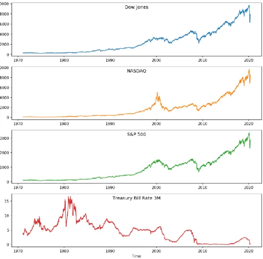
The dataset we are going to use includes: Dow Jones, NASDAQ and Standard & Poor’s 500 market indexes and the 3 month Treasury bill rate, sampled weekly, as can be observed in Figure 1. The data were cut short in time domain so that every series spaned over the same time period. All market indexes are the closing price on every Friday of the month and luckily the treasury bill rate was also available on the same day so no resampling or data shifting was required.

After collecting the data from the Reuter-Thomson Datastream platform (Reuters-Thomson, 2020) we test all time series for stationarity by using the Augmented Dickey–Fuller unit root test (ADF) (Dickey & Fuller, 1979; Dickey & Fuller, 1981). This test indicates that the four time series are non-stationary with p-values well above 5% significance level (0.9945, 0.9989, 0.9959, 0.6274). The log-returns are stationary (based on ADF test), which is conducent to a VECM analysis, on the assumption that cointegration exists. From this point on, all numerical results presented in the text in the form of 4-tuples are related to each of the variables in the order presented in Figure 1.

Figure 1. Macroeconomic variables and stock indexes in study.

We establish two major datasets: the training set for the VECM estimation and a test set which we use to benchmark VECM’s prediction capabilities as well as to supply the input for the LSTM algorithm to effectively “correct”. The training dataset runs from 5 of February 1971 until 12 of May 2013 while test set goes from 19 of May 2013 until 17 of April 2020. In the VECM model fitting procedure we minimize Akaike Information Criteria (AIC) in order to determine the optimal lag, which in this case is of 2 time steps (weeks in our time binning). The cointegration was detected by adopting the Johansen methodology (Johansen, 1988; Johansen, 1992) where both trace and maximum eigenvalue tests conclude that exist three cointegration vectors for the optimal lag order of 2.

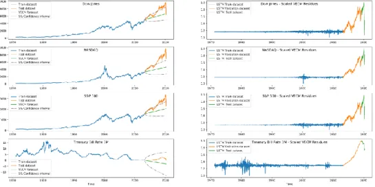
After the model was established we use the VECM(2) with 3 cointegration vectors to estimate the parameters and to extract the residuals (for the training set) and to forecast (for the test set). Note that these residuals were then scaled in order to comply with the LSTM network which will use them as input. These results can be found in Figure 2.

Figure 2. VECM model applied to data (left) and the corresponding residuals (right).

We estimated an average percentual deviation of the VECM model from data in the training sample given by (1.489%, 0.901%, 2.234%, 1.196%). The prediction results based on VECM, ilustrated in Figure 2, strongly deviate from the data as time passes but this was to be expected given the extremely long prediction range (about 7 years), resuming to only predict the global trend.

2.2. LSTM network

After the residuals were extracted and scaled to a 0 to 1 grading, we introduce them as input in our LSTM network.

We split the “forecast” dataset of the VECM into two subsets in order to create a “validation” and a new “test” datasets for the LSTM’s training and benchmarking. The new time intervals splits are given by: 1971-02-19 to 2013-04-12 for training, 2013-04-19 to 2019-04-12 for validation and 2019-04-19 to 2020-04-17 for testing.

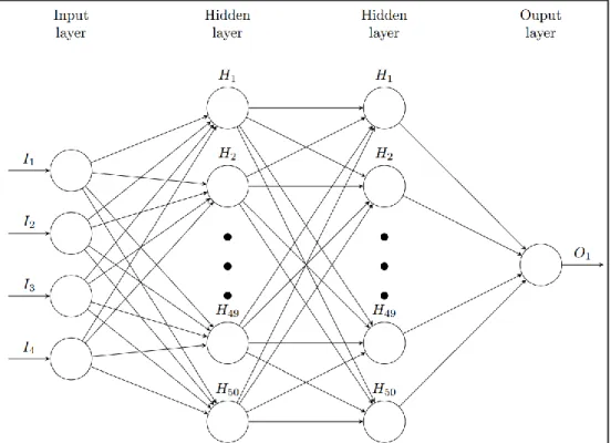
This network’s configuration, presented in Figure 3 (namely the number of time steps, batch size, training epochs and hidden layer configuration) came from a long run of trial and error.

Figure 3. Diagram of the LSTM Recurrent Neural Network deployed.

Table 1 synthesize the different parameters that define our LSTM arquitecture. We use Keras and Tensorflow from Python. In order to normalize the data we use the MinMaxscaler, which scales and translates each feature individually such that will belong to the given range on the training set, e.g. between zero and one. To avoid using Sigmoid functions, ReLU (Rectified Linear Unit) activation functions became a popular choice in deep learning and even nowadays provides outstanding results. An optimizer is one of the two arguments required for compiling a Keras model. We used Adam, an algorithm for first-order gradient-based optimization of stochastic objective functions, based on adaptive estimates of lower-order moments. Finally, we present the values exploit for the number of time steps, hidden layers, learning rate, batch size and training epochs.

2.3. Results

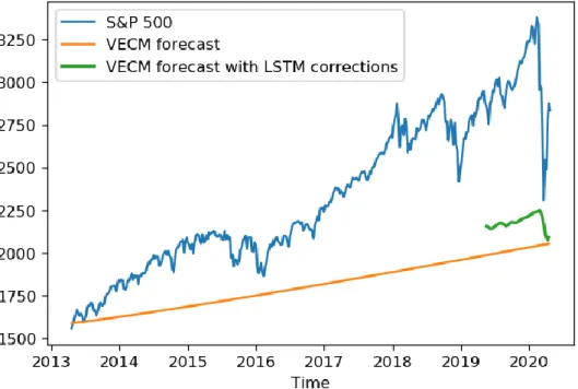
After training, the network was used to predict the residuals of the time series in order to correct the VECM forecasts. This was merely done by adding the LSTM prediction to the VECM prediction after the scaling was inverted.

The results are presented in Figure 4. The average percentual deviation of this approach from the data is 28.192%.

Table 1. LSTM architecture.

Data normalization MinMaxScaler

Activation function ReLU

Optimizers Adam

Loss Function Mean Squared Error

Input dimension 4 (timestep) x 4

Output dimension 1 (forecast)

Hidden layers [50, 50]

Learning rate 1.E-3

Batch Size 32

Figure 4. VECM prediction and the VECM with LSTM correction.

The LSTM’s additive correction introduced some temporal variation but it was not able to correct for such a large shift from the forecast to the data. This shortage can be attributed to the discrepant change in the behaviour of the residual dataseries presented in Figure 2.

3. Conclusions and Prospects

The approach of making an unbiased long term “trend” prediction of the different time series and then attempting to correct them using an LSTM network proved to be difficult. The residual series sharply change and the LSTM was not able to take that into account during its training since only a simple residual series was provided. This conduces to the introduction of two new objectives in future analysis, namely, an adjustment in the forecasting range and a change in the training philosophy.

This model yielded a MAPE of 28.192% when prediciting the Standard & Poor’s stock market index. This might be attributed to the usage of a relatively small dataset.

We plan to expand this analysis to daily data but that will constrain our choices due to data availability of macroeconomic variables on these high frequency samplings.

References

Dickey, D. A., & Fuller, W. A. (1979, June). Distribution of the Estimators for Autoregressive Time Series With a Unit Root. Journal of the American Statistical Association, 74(366). doi:10.2307/2286348

Dickey, D. A., & Fuller, W. A. (1981, Jul). Likelihood Ratio Statistics for Autoregressive Time Series with a Unit Root. Econometrica, 49(4), pp. 1057-1072. doi:10.2307/1912517 Engle, R. F., & Granger, C. W. (1987, Mar). Co-Integration and Error Correction: Representation, Estimation, and Testing. Econometrica, 55(2), pp. 251-276. doi:10.2307/1913236

Fischer, T., & Krauss, C. (2017). Deep learning with long short-term memory networks. FAU Discussion Papers in Economics. doi:10.1016/j.ejor.2017.11.054

Johansen, S. (1988). Statistical analysis of cointegration vectors. Journal of Economic Dynamics and Control, 12(2-3), pp. 231-254. doi:10.1016/0165-1889(88)90041-3 Johansen, S. (1992, June). Cointegration in partial systems and the efficiency of

single-equation analysis. Journal of Econometrics, 52(3), pp. 389-402. doi:10.1016/0304-4076(92)90019-N

Kim, H., & Won, C. H. (2018, Aug). Forecasting the volatility of stock price index: A hybrid model integrating LSTM with multiple GARCH-type models. Expert Systems with Applications, 103, pp. 25-37. doi:10.1016/j.eswa.2018.03.002

Mills, T. C., & Markellos, R. N. (2008). The Econometric Modelling of Financial Time Series. Cambridge University Press. doi:10.1017/CBO9780511817380

Nelson, D. M., Pereira, A. C., & Oliveira, R. A. (2017, May). Stock market's price movement prediction with LSTM neural networks. International Joint Conference on Neural Networks (IJCNN) (pp. 1419-1426). IEEE. doi:10.1109/IJCNN.2017.7966019

Reuters-Thomson. (2020). Datastream. Retrieved from

https://www.refinitiv.com/en/products/datastream-macroeconomic-analysis/

Terui, N., & van Dijk, H. K. (2002). Combined forecasts from linear and nonlinear time series models. International Journal of Forecasting(18), pp. 421-438. doi:10.1016/S0169-2070(01)00120-0

Wan, H., Guo, S., Yin, K., Liang, X., & Lin, Y. (2020, March 5). CTS-LSTM: LSTM-based neural networks for correlatedtime series prediction. Knowledge-Based Systems, 191. doi:10.1016/j.knosys.2019.105239

Zhang, G. P. (2003, Jan). Time Series Forecasting Using a Hybrid ARIMA and Neural Network Model. Neurocomputing, 50(17), pp. 159-175. doi:10.1016/S0925-2312(01)00702-0

Zhang, G. P., & Qi, M. (2005, Feb). Neural network forecasting for seasonal and trend time series. European Journal of Operational Research, 160(2), pp. 501-514. doi:10.1109/TNN.2007.912308