Abstract—Single-objective bilevel optimization is a specialized form of constraint optimization problems where one of the constraints is the optimization problem itself. These problems are typically non-convex and strongly NP-Hard. Recently, there has been an increased interest from evolutionary computation community to model bilevel problems due to its applicability in the real world applications for decision-making problems. In this work, we are utilizing a partial nested evolutionary approach with local heuristic search to solve the benchmark problems and have outstanding results. This approach relies on the concept of intermarriage-crossover in search for feasible regions by exploiting information from the constraints. We are also proposing new variants to the commonly used convergence approaches, i.e., optimistic and pessimistic. The experimental results demonstrate the algorithm converges differently to known optimum solutions with the optimistic variants. Optimistic approach also outperforms pessimistic approach. Comparative statistical analysis of our approach with other recently published partial to complete evolutionary approaches demonstrates very competitive results.
Index Terms—bilevel optimization, evolutionary computation, intermarriage-crossover, optimistic and pessimistic, decision-making
1. INTRODUCTION
Optimization problems are very common in many fields such as engineering, operations research, economics, and games, to get the most favorable solution from a feasible set of solutions. Bilevel optimization problem is structured as a nested optimization problem in the form of constraint optimization problem (COP) where a solution must satisfy a set of constraints. These constraints can be either scalar/vector or static/dynamic functions [18]. In bilevel problems, one or more constraints are the COP themselves. This makes bilevel programming combinatorial and strongly NP-hard [8, 9]. Bilevel programming was motivated by [28] who used game theory to solve unbalanced economic market problem with multilevel optimization. Here, upper-level is called the leader and the lower-level is called the follower. The earliest formalization of bilevel problem using mathematical programming was published in [3] where bilevel problem was called two-sided optimization with outside optimizer and inside optimizer in a hierarchical setup.
Bilevel problem formulations employ either optimistic or pessimistic convergence approach where both have different selection criteria for selecting promising solutions; consequently, they result in different convergence [27, 29, 33, 34]. We have analyzed these convergence strategies in this paper and proposed new variants for better convergence for selected problems. Recently, there has been an increase in interest in solving bilevel optimization problem where many new classical and evolutionary approaches have been proposed [5, 7, 10, 22–27]. We concisely describe some commonly used methodologies for solving bilevel problems in the following section. Readers may find the detailed survey in [5, 27, 31].
A commonly used approach in mathematical programming is to convert bilevel optimization problem into a single level COP with Karush-Kuhn-Tucker (KKT) conditions, however, it may not necessarily be simple to handle especially when the upper-level’s constraint functions are in an arbitrary linear form [2, 22]. Another commonly used approach is the penalty function methods where constraints are transformed into penalty terms, which in turn are used for reward and/or punishment for satisfying and/or violating the constraints, respectively [32]. However, its main shortcoming is that penalty factors that determine the severity of the punishment must be set by the user and their values are problem dependent [19]. Similar to penalty functions, a trust region method uses an initial approximation of a trust-region that expands (reward) if the approximation is good or contracts (punishment) otherwise. This can be called an iterative guided approach through trust-regions [13]. Another iterative reduction of approximation error is done with gradient descent approach [16]. The direction of descent leads towards optimization (least error) of the upper-level function while keeping the lower-upper-level feasible. Gradient descent is commonly used in machine learning algorithms [1].
Finally, Evolutionary Algorithms (EAs) have also been used either in upper-level or both levels of bilevel problems [11, 14]. EAs are known to give reasonable solutions for NP-Hard optimization problems and they have been successfully applied to various forms of COPs [18]. Li et al. [11] have proposed a hierarchical particle swarm optimization for solving bilevel programming
Optimistic Variants of Single-Objective Bilevel
Optimization for Evolutionary Algorithms
Anuraganand Sharma
(HPSOBLP) that simulates the decision process of bilevel programming on both levels using Particle Swarm Optimization. However, this technique may have high time complexity because of the nested nature of the algorithm. Recently, some hybrid approaches of EAs with other mathematical techniques have been proposed in [26] and [10] where upper level is an EA and lower level is a local search. Sinha and Deb [23–27] have done an extensive work for evolutionary bilevel problems. They have proposed a Bilevel EA based on quadratic approximation (BLEAQ) that reduces the bilevel optimization problem to a single level optimization problem using quadratic functions [26]. They have also prepared a set of ten benchmark problems from the literature [26]. Kieffer et al. [10] have used Differential Evolution based Bayesian Optimization for Bilevel Problems (BOBP). BOBP has focused more on efficiency of the algorithm that also shows competitive results compared to BLEAQ.
Bilevel problem can have either single-objective optimization (SOO) or multi-objective optimization (MOO) for both the levels. We have focused on SOO for both the levels in this paper where a variation of EA has been applied to various convergence methodologies described for bilevel problems. For rest of the paper, we will refer single-objective bilevel optimization problem as bilevel problem only. We have enhanced Intelligent Constraint Handling Evolutionary Algorithm (ICHEA) [18, 19] that uses intermarriage-crossover twice in a generation; once each for both the levels of bilevel problems unlike BLEAQ, BLOP and HPSOBLP. ICHEA was designed to solve static and dynamic constraints effectively [18–21], however, it was never tested for a bilevel problem which is a special kind of COP. The enhanced ICHEA uses an evolutionary approach at the upper level and heuristic local search at the lower level with very promising test results. We have used ICHEA to analyze various kinds of convergence approaches on benchmark bilevel problems. The remainder of this paper is organized as follows: Section 2 describes the mathematical formulation of bilevel problems. Section 3 establishes the existing and our proposed variants for convergence techniques applicable for bilevel problems. Section 4 formalizes and describes the complete evolutionary approach to solve bilevel problems with ICHEA. Section 5 elaborates experimental results of our approach with three other recent partial and complete evolutionary approaches on benchmark problems and Section 6 concludes the paper by proposing future investigations.
2. FORMULATION OF BILEVEL PROBLEMS
Generally, a Bilevel problem is a two-level nested constraint optimization problem (COP). Hence, we initially define the formulation of COP. A COP is simply an optimization problem with a set of constraints. We have assumed that both levels are minimization problems for simplicity. Eq. (1) is minimization of COP’s objective function ݂ሺݔԦሻ that has an ݊-dimensional input vector ݔԦ ൌ ሼݔଵǡ ݔଶǡ ǥݔሽ that is defined in a search space ܵ.
݂ሺݔԦሻ
More specifically, ݔԦ א ࣠ ك ܵ, where ࣠ being the feasible region on the search space ܵ ك Թ. The domain of variables is defined by their lower bounds ݈ and upper boundsݑ:
݈ ݔݑǡͳ ݅ ݊
The feasible region ࣠ with bounds on each dimension is further restricted by a set of ݉ additional constraints that can be given in two relational forms – equality and inequality [6, 12, 17, 30].
݃ሺݔԦሻ Ͳ݅ ൌ ͳǡ ǥ ǡ ݇
݄ሺݔԦሻ ൌ Ͳ݆ ൌ ݇ ͳǡ ǥ ǡ ݉
The equality constraints ݄ሺݔԦሻ cannot be solved directly using EAs so it is converted into inequality constraints by introducing a positive tolerance value ߜ.
݃ሺݔԦሻ ൌ ߜ െ ห݄ሺݔԦሻห Ͳ
A set of individual feasible regions ሼ࣠ଵǡ ࣠ଶǡ Ǥ Ǥ ࣠ሽ for each constraint can also be defined as:
࣠ൌ ሼݔԦ א ࣠ȁ݃ሺݔԦሻ Ͳǡ ͳ ݅ ݉ǡ ݅ א ܼሽ
where ܼ is the set of integers. Many EAs use a distance function as their fitness function to rank individuals. The distance function indicates how far a chromosome is from the feasible region [15]. This fitness function tries to bring the chromosomes closer to the feasible region using the following function for݅ ሼͳ ݅ ݉ሽ:
݂݅ݐ݊݁ݏݏሺݔԦሻ ൌ൜݃Ͳǡ݂݅݃ሺݔԦሻǡ݂݅݃ሺݔԦሻ ൏ Ͳ
ሺݔԦሻ Ͳ
The fitness function ݂݅ݐ݊݁ݏݏ in Eq. (7) is a measure of infeasibility of ሬԦ from a feasible region ࣠୧. The error function ݁ is the summation of all the fitness functions as shown in Eq. (8). Minimizing the error value݁ leads toward a constraint satisfaction problem’s (CSP) solution where the objective function ݂ሺݔԦሻ is not needed. A solution to CSP is found when݁ ൌ Ͳ or ځ ࣠ୀଵ ് . To get a COP solution, CSP solutions are further processed to get optimum value of ሬԦ that optimizes the objective function ݂ሺݔԦሻ.
Bilevel problem is simply a hierarchical set up of nested COP where the upper level is commonly known as the leader while the lower level is known as the follower. We have used the same variable names discussed above only with addition of subscripts ݑ andݒ to indicate upper and lower level, respectively. The formulation is described below:
ܨሺݔԦ௨ǡ ݔԦሻ Such that: ௫Ԧ ܩଵ ሺݔԦ௨ǡ ݔԦሻ Such that: ݃ሺݔԦ௨ǡ ݔԦሻ Ͳ݅ ൌ ͳǡ ǥ ǡ ݇ ݄ሺݔԦ௨ǡ ݔԦሻ ൌ Ͳ݆ ൌ ݇ ͳǡ ǥ ǡ ݉ ܩሺݔԦ௨ǡ ݔԦሻ Ͳ݅ ൌ ʹǡ ǥ ǡ ݇௨ ܪሺݔԦ௨ǡ ݔԦሻ ൌ Ͳ݆ ൌ ݇௨ ͳǡ ǥ ǡ ݉௨
where ܨሺݔԦ௨ǡ ݔԦሻ is the upper level objective function with ݉௨ constraints that has one constraint in the form of lower level objective function given as
௫Ԧ ܩଵሺݔԦ௨ǡ ݔԦሻǤ
It is generally written as
௫Ԧ ݂ሺݔԦ௨ǡ ݔԦሻ
to be consistent with the upper level objective function [5, 10, 27].
3. VARIANTS OF CONVERGENCE TECHNIQUES FOR BILEVEL PROBLEMS
Two widely discussed optimization variants are the optimistic and the pessimistic models [27, 29, 33, 34]. We discuss these variants with our proposed variants that an EA can use in a given generation in the following section. These variants demonstrate variable extent of greediness in their choice for selecting a solution. The population converges differently with these strategies demonstrated in Section 5.
3.1. Optimistic w.r.t upper level (OF)
In this greedy approach, the follower altruistically chooses a feasible solution that benefits the leader the most. ȲሺݔԦ௨ሻ ൌ ቊݔԦǣ ݔԦא
௫Ԧ ݂ሺݔԦ௨ǡ ݔԦሻ ǣ ሺݔԦ௨ǡ ݔԦሻ א ࣠ቋ If ȲሺݔԦ௨ሻ is not a singleton then:
Ȳ୭ሺݔԦ௨ሻ ൌ ቊݔԦא
௫Ԧ ܨሺݔԦ௨ǡ ݔԦሻǣ ݔԦא ȲሺݔԦ௨ሻቋ
Again, we may not get a singleton set but the “best” is picked at random. The overall optimistic model w.r.t upper level can be defined as:
ܨሺݔԦ௨ǡ ݔԦሻ Such that:
ݔԦൌ Ȳ୭ሺݔԦ௨ሻ ሺݔԦ௨ǡ ݔԦሻ א ࣠௨
To illustrate further, a numerical example is given in TABLE I, which shows sample fitness values for a given ݔԦ௨ and its corresponding parameter ݔԦ where ݅ ൌ ͳ ǥ5. The minimum lower level fitness is 100 and the corresponding minimum upper level fitness is 22. Hence, OF approach will result in the selection of ሺݔԦ௨ǡ ݔԦమሻ.
SAMPLE DATA FOR CONVERGENCE VARIANTS
݂ሺݔԦ௨ǡ ݔԦሻ ܨሺݔԦ௨ǡ ݔԦሻ PF→ ݔԦ௨ǡ ݔԦభ 100 25 OF→ ݔԦ௨ǡ ݔԦమ 100 22 ݔԦ௨ǡ ݔԦయ 100 23 ݔԦ௨ǡ ݔԦర 112 11 ← EOF ݔԦ௨ǡ ݔԦఱ 115 50
Conversely, the other variant for optimistic w.r.t lower level (Of) can also be easily formulated where a solution chosen by the
3.2. Pessimistic w.r.t upper level (PF)
On this convergence approach, the follower shows no cooperation to the leader and gives the worst feasible solution from the lower level.
ȲሺݔԦ௨ሻ ൌ ቊݔԦǣ ݔԦא
௫Ԧ ݂ሺݔԦ௨ǡ ݔԦሻ ǣ ሺݔԦ௨ǡ ݔԦሻ א ࣠ቋ If ȲሺݔԦ௨ሻ is not a singleton then:
Ȳ୮ሺݔԦ
௨ሻ ൌ ቊݔԦא
௫Ԧ ܨሺݔԦ௨ǡ ݔԦሻǣ ݔԦא ȲሺݔԦ௨ሻቋ The complete pessimistic PF model would be:
ܨሺݔԦ௨ǡ ݔԦሻ Such that:
ݔԦൌ Ȳ୮ሺݔԦ௨ሻ ሺݔԦ௨ǡ ݔԦሻ א ࣠௨
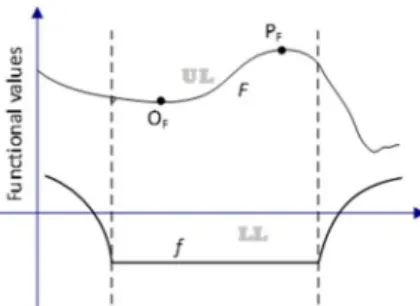
In TABLE I, the worst feasible solution for the upper level would be produced by parametersݔሬሬԦ௨ǡ ݔԦభ. Fig.1 illustrates the difference between OF and PF when ȲሺݔԦ௨ሻ is not a
singleton.
Wiesemann et al. [33] has defined that the follower may choose to give any possible feasible solution not necessarily the best or the worst. In this case:
Ȳ୮ሺݔԦ
௨ሻ ൌ ሼݔԦא ȲሺݔԦ௨ሻሽ
In this variant, a set of solutions for PF in TABLE I would be ሺݔԦ௨ǡ ݔԦሻwith ݅ ൌ ͳ ǥ 3 where any one of the solution can be
picked randomly.
3.3. Extreme optimistic w.r.t upper level (EOF)
In this extremely greedy model, w.r.t upper level, the follower blindly chooses a partially feasible solution ൫ݔԦ௨ǡ ݔԦכ൯ that benefits the leader the most, disregarding the other more promising solutions available for himself at a given generation. However, the chosen lower level solution should not be worse than the previously found lower level solution in anticipation that optimum solution may be found later on.
ȳሺݔԦ௨ሻ ൌ ൛ݔԦכǣ ݂൫ݔԦ௨ǡ ݔԦכ൯ ݂ሺݔԦ௨ǡ ݔԦሻǣ ሺݔԦ௨ǡ ݔԦכሻ א ࣠െ ࣠భൟ
where ݔԦכ and ݔԦ are the solutions of current and previous generations, respectively. ࣠భis a feasible region produced by the lower level optimization function. If ȳሺݔԦ௨ሻ is not a singleton then:
ȳୣ୭ሺݔԦ௨ሻ ൌ ቊݔԦא
௫Ԧ ܨሺݔԦ௨ǡ ݔԦሻǣ ݔԦא ȳሺݔԦ௨ሻቋ
In this case, we may not get a singleton set so we pick the “best” at random. The overall extreme optimistic model w.r.t upper level can be defined as:
ܨሺݔԦ௨ǡ ݔԦሻ Such that:
ݔԦൌ ȳୣ୭ሺݔԦ௨ሻ ሺݔԦ௨ǡ ݔԦሻ א ࣠௨
According to TABLE I, sample data ሺݔԦ௨ǡ ݔԦరሻ will be picked for EOF if previous lower level fitness is more than or equal to 112.
4. BILEVEL PROBLEM OPTIMIZATION WITH ICHEA
ICHEA, which is a variation of EA, is an effective and versatile constraint handling tool that has been demonstrated to perform well for benchmark static and dynamic continuous CSPs in [19, 20] and COPs in [18, 21]. ICHEA uses intermarriage-crossover operator that uses knowledge from constraints rather than blindly searching for the solution. In this particular crossover, both parents belong to different feasible regions ࣠ and ࣠ where݅ ് ݆. It is also possible that a parent does not belong to any of the feasible regions ܵ െ ܨ. These parents are made to come closer towards the boundary of their corresponding feasible regions to locate the overlapping regions that results in more constraints being satisfied. This iterative move can be captured as:
ܱଵൌ ݎሺܲଶെ ܲଵሻ
Fig. 1. A sketch to illustrate optimistic and pessimistic conditions w.r.t. upper-level
where offspring ܱଵ is initially placed at position ݎଵሺܲଶെ ܲଵሻ which is then iteratively moved closer to parent ܲଵ until it also satisfies the constraint(s) that ܲଵ satisfies and similarly offspringܱଶ is designated. ݎ is a coefficient in the range ሺͲǡ ͳሻ which is generally 0.5 that gives binary traversal for convergence. Exponent ݅ gets incremented from 1 to a threshold value ܶin the sequenceۃͳǡʹǡ Ǥ Ǥ Ǥ ǡ ܶۄ. ܶ is proportional to the “vastness” of the search space which is generally ʹ. The intermarriage-crossover process is shown in Fig. 2 where 3 mark indicates possible placement for an offspring and × mark indicates the offspring vector is unacceptable in that particular position. The generated offspring from intermarriage-crossover contains genes from both parents. The purpose is to make a “generic” offspring who tries to satisfy more constraints because his parents are from two different feasible regions. The algorithm favors those offspring who satisfy more constraints by utilizing Deb’s ranking scheme based on feasibility [6] to rank the individuals. The population is first sorted according to number of satisfied constraints in decreasing order then by fitness value in increasing order. The worst time complexity of this crossover is the same as the time complexity of an individual objective function evaluation ܱሺܾ݆ܨݑ݊ܿሻ i.e. ܱሺʹ ൈ ܶ ൈ ܾ݆ܨݑ݊ܿሻ ൌ ܱሺܾ݆ܨݑ݊ܿሻ.
Fig. 2. Intermarriage-Crossover between parents P1 and P2
The details of complete ICHEA algorithm for bilevel problem, called Bilevel ICHEA (BICHEA) is given in Fig. 3. It has a partial nested approach where evolutionary algorithms (ICHEA) is at the upper level and local search (mutation of clones with intermarriage-crossover) at the lower level. The rest of the structure does not deviate much from the original ICHEA. BICHEA can be described in four major steps:
Step1: The algorithm starts with the initialization of a set of chromosomes ܥ that evolves for a given number of generations. Each chromosome contains upper and lower level input parameters, current fitness values and information about the given constraints being violated.
Step 2: this is a nested local search step where search for more promising lower level parameters happen. Here all feasible chromosomes go through exploitation process of hyper mutation with localSearch defined in Fig. 4. localSearch applies the optimistic convergence technique for sectors ܵଶ and ܵଷ and extreme-optimistic otherwise. We have also tried to use different orders for convergence techniques but the outcome remains same. Subroutine clone uses the concept of hyper-clone defined in [4]. It merely creates ൬ͳͲǡ ݈ܿ݁݅ ቀఉǤԡԡ ቁ൰number of clones in proportion to the order of fitness given by ݅ א ሼͳǡ ǥ ǡ ԡܥԡሽ and constant parameter ߚ which has been set to 0.5 for this work. Here intermarriage happens between a given chromosome with a randomly generated boundary values. For a given individual ܲ with parametersሺݔԦ௨ǡ ݔԦሻ, ݔԦ௨ is fixed for the lower-level to get the most suitable ݔԦ. Intermarriage-crossover creates a clone ܲԢ for this individual that replaces ݔԦ with its boundary values. Boundary value B for a variable ݔԦǣ ͳ ݅ ԡݔԦԡ is either lower bound or upper bound denoted byܤሺݔԦሻ ൌ ݉݅݊ሺݔԦሻ and ܤ௫ሺݔԦሻ ൌ ݉ܽݔሺݔԦሻ, respectively. We randomly pick the minimum or maximum for each variable in a vector ݔԦ given by ሺݔԦሻ. Now the distance ߜ between ܲ and ܲԢ is:
ߜ ൌ ฯݔԦ௨ ݔԦ൨ െ ݔԦ ௨ ሺݔԦሻ൨ฯ ൌ ԡݔԦെ ሺݔԦሻԡ൨
ܲ move towards ܲԢ in a hyper-plane to search for the local best solution. If the boundary values are not given, then any large value such as േͳͲܧͶ can be used instead.
Step 3: this is the upper level search with Intermarriage-crossover (interMarCrossover) which tries to explore for more promising chromosomes (based on a given convergence strategy) without fixing any of the parametersሺݔԦ௨ǡ ݔԦሻ contrary to Step 2. This step is necessary to get diverse individuals in a population [21].
Step 4: lastly, SortAndDiscard filters out promising chromosomes based on given sectors with either upper level objective function F or lower level objective function f. ܵଵെ ܵସ divides the total generations in order from first to fourth sectors. Here promising solutions are selected based on a given convergence strategy which causes different convergence for each sector. Sectors ሼܵଵǡ ܵଶሽ and ሼܵଷǡ ܵସሽ sort the population w.r.t upper level fitness, and lower level fitness respectively.
Feasible Region ښi Feasbile Region ښj Parent P1 Parent P2 Offspring O1 Offspring O2 9 × 9
Function BICHEA(problem, Generations)
ܥ ൌ initializeChromosomes(problem);
For each ݃ אGenerations
ܥ = localSearch(ܥǡ ݃);
ܲ = tournamentSelection(ܥ);
ܱ = interMarCrossover(ܲ);
ܥ ൌ ܥ ܱ;
sortBy = ݃ א ሼܵଵ ܵଶሽǫ byF : byf;
ܥ = SortAndDiscard(ܥ, sortBy);
PrintBest5(ܥ);
CheckTerminationCriteria(); End For
End Function
Fig. 3. Pseudocode for BICHEA Function ܥᇱൌlocalSearch(ܥǡ ݃) ܥᇱൌ For each ܿ א ܥ ܪ = clones(ܿ); ܪԢ ൌ For (each ݄ א ܪ) ݄’= InterMarCrossover(݄,aBoundaryOf(݄)); ܪԢ ൌ ݄Ԣ ܪԢ End for
model = ݃ א ሼܵଶ ܵଷሽǫ Optimistic : extreme Optimistic;
ܪԢ = sort(ܪԢ, model);
ܥᇱൌ ܥᇱ ܪᇱ.getBest();
End for
Return ܥᇱ; End Function
Fig. 4. Pseudocode for subroutine blMutation 5. EXPERIMENTS AND DISCUSSION
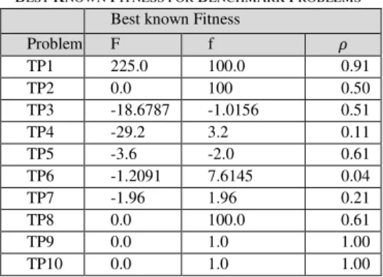
BICHEA has been tested on ten standard benchmark bilevel problems from [10, 26] to evaluate its performance with other recently developed evolutionary approaches discussed in Section 1. TABLE II describes the best known fitness values for upper level (F) and lower level (f). The problem set includes combination of linear and non-linear functions with mostly small dimensional problems with weak constraint strengths (ߩ) apart from lower level constraint. This shows that feasible regions can be identified almost immediately. ߩ is computed offline by using the formula ߩ ൌ ȁȁ ȁȁΤ randomly. We used a population size of 10,000 to determine the ߩ value as the average of five successive runs [12, 20].
BEST KNOWN FITNESS FOR BENCHMARK PROBLEMS
Best known Fitness
Problem F f ߩ TP1 225.0 100.0 0.91 TP2 0.0 100 0.50 TP3 -18.6787 -1.0156 0.51 TP4 -29.2 3.2 0.11 TP5 -3.6 -2.0 0.61 TP6 -1.2091 7.6145 0.04 TP7 -1.96 1.96 0.21 TP8 0.0 100.0 0.61 TP9 0.0 1.0 1.00 TP10 0.0 1.0 1.00
BEST FITNESS COMPARISON
BICHEA Bayesian BLEAQ HPSOBLP
Prob F f F f F f F f TP1 225.00009 99.99968 225.001199.9984 225.0 100.0 225 100 TP2 0.00003 199.99971 0.0 200.0 5.4204 0.0 0 100 TP3 -18.67869 -1.01559 -18.6786 -1.0156 -18.6787 -1.0156-14.8 0.21 TP4 -29.19869 3.19633 -29.1991 3.2001 -29.2 3.2 -36.0 0.25 TP5 -3.67982 -2.01346 -3.8998 -2.0039-2.4828 -7.705 - - TP6 -1.20918 7.61450 -1.2099 7.6173 -1.2099 7.6173 - - TP7 -1.96001 1.96001 -1.6833 1.6833 -1.8913 1.8913 - - TP8 0.00000 100.000000.0 200.0 12.2529 0.0007 - - TP9 0.00000 1.00000 0.0007 1.0 3.5373 1.0 - - TP100.00000 1.00000 0.0011 1.0 0.001 1.0 - -
AVERAGE FITNESS COMPARISON
BICHEA Bayesian BLEAQ HPSOBLP
Prob F f F f F f F f TP1 224.96290 99.99192253.6155 70.3817 224.9989 99.9994 225 - TP2 0.00012 199.99890.0007 183.871 2.4352 93.5484 0 - TP3 -18.67862 -1.01533-18.5579 -0.9493 -18.6787 -1.0156 -14.0 - TP4 -29.159662.66120 -27.6225 3.3012 -29.2 3.2 -36.0 - TP5 -4.26669 -1.99426 -3.8516 -2.2314 -3.4861 -2.569 - - TP6 -1.21052 7.61467 -1.2097 7.6168 -1.2099 7.6173 - - TP7 -1.96173 1.96173 -1.6747 1.6747 -1.9538 1.9538 - - TP8 0.36679 92.69204 0.0008 180.645 1.1463 132.559 - - TP9 0.00000 1.00000 0.0012 1.0 1.2642 1.0 - - TP100.00000 1.00000 0.0049 1.0 0.0001 1.0 - -
BEST FITNESS STATISTICS FOR BICHEA
Prob F Variance for F f Variance for f
TP1 225.00009 0.033 99.99968 0.077 TP2 0.00003 0.000 199.99971 0.002 TP3 -18.67869 0.000 -1.01559 0.000 TP4 -29.19869 0.122 3.19633 0.174 TP5 -3.67982 0.621 -2.01346 1.034 TP6 -1.20918 0.000 7.61450 0.000 TP7 -1.96001 0.000 1.96001 0.000 TP8 0.00000 5.204 100.00000 834.887 TP9 0.00000 0.000 1.00000 0.000 TP10 0.00000 0.000 1.00000 0.000
PARAMETER SETTINGS FOR BICHEA
Parameters Values Population size 100 Generations 500 (S1: 1-125; S2: 126-250; S3: 251 – 375; S4: 376 – 500) T 2 ߚ 0.5 blMutation rate 1.0 Crossover rate 0.8 Runs 30/problem
Fig. 5. Fitness accuracy of best found solutions Ϭ Ϭ͘ϬϮ Ϭ͘Ϭϰ Ϭ͘Ϭϲ Ϭ͘Ϭϴ Ϭ͘ϭ /, ĂLJƐĞŝĂŶ >Y ,W^K>W /, ĂLJƐĞŝĂŶ >Y ,W^K>W /, ĂLJƐĞŝĂŶ >Y ,W^K>W /, ĂLJƐĞŝĂŶ >Y ,W^K>W /, ĂLJƐĞŝĂŶ >Y ,W^K>W /, ĂLJƐĞŝĂŶ >Y ,W^K>W /, ĂLJƐĞŝĂŶ >Y ,W^K>W /, ĂLJƐĞŝĂŶ >Y ,W^K>W /, ĂLJƐĞŝĂŶ >Y /, ĂLJƐĞŝĂŶ >Y /, ĂLJƐĞŝĂŶ >Y /, ĂLJƐĞŝĂŶ >Y /, ĂLJƐĞŝĂŶ >Y /, ĂLJƐĞŝĂŶ >Y /, ĂLJƐĞŝĂŶ >Y /, ĂLJƐĞŝĂŶ >Y /, ĂLJƐĞŝĂŶ >Y /, ĂLJƐĞŝĂŶ >Y /, ĂLJƐĞŝĂŶ >Y /, ĂLJƐĞŝĂŶ >Y & Ĩ & Ĩ & Ĩ & Ĩ & Ĩ & Ĩ & Ĩ & Ĩ & Ĩ & Ĩ d W ϭ d W Ϯ d W ϯ d W ϰ d W ϱ d W ϲ d W ϳ d W ϴ d W ϵ d W ϭ Ϭ ĞǀŝĂƚŝŽŶ ĞƐƚ&ŝƚŶĞƐƐĐĐƵƌĂĐLJŽŵƉĂƌŝƐŽŶ
Parameter settings for BICHEA is shown in TABLE III where S1-S4 indicates four equal sectors with given ranges to test different convergence approaches. Sectors S1 with generations 1-125, S2 with generations 126-250, S3 with generations 251-375 and S4 with generations 276-500 have been used to test convergence approaches EOF, OF, Of and EOf respectively. In case, a finite
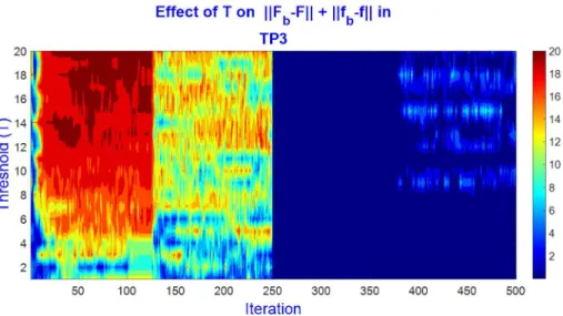
range for a variable is not defined, we used upper/lower limit of value ±10,000.00. Overall, each problem was executed 30 runs consecutively to have a comparative analysis with the published results of BLEAQ, Bayesian and HPSOBLP from [10, 11]. Value of parameter ܶ can be adaptive but currently a constant value 2 has been used as it gives more promising results compared to other values. Fig. 6 shows the behavior of ܶ on the quality of solutions i.e. (ȁܨ െ ܨȁ ȁ݂ െ ݂ȁ), where ሼܨǡ ݂ሽ are known optimum solutions. The higher values shows degradation in the quality of the solutions which are also inefficient as the computations increases many folds for intermarriage crossover.
TABLE IV and TABLE V show the list of best and average results, respectively from all the tested algorithms. Bold values indicate the best (or almost best) among the tested algorithms and ‘-’ indicates the unavailability of the result. BICHEA has also produced competitive results when only average fitness is considered, however, it has performed very well for best fitness values for all the testing problems except for lower level fitness in problems TP2 and TP5. For most of the problems, BICHEA has found the known best solutions. Fig. 5 shows the deviation of the best found solution ሼܨǡ ݂ሽ from known optimum solutions ሼܨǡ ݂ሽ i.e. ȁܨെ ܨȁ for upper level and ȁ݂െ ݂ȁ for lower level. Deviation of more than േͲǤͳ is considered an unacceptable solution, thus terminated to 0.1. BICHEA shows very few or smaller bars of deviation compared to the other algorithms. Overall, BICHEA performs almost equally well for most of the problems in every test runs with low variations as shown in TABLE VI. Only TP8 and somewhat TP5 do not show consistency with high variance which is also observed in TABLE V for average result.
Fig. 6. Analysis on the values of threshold T w.r.t the quality of a solution
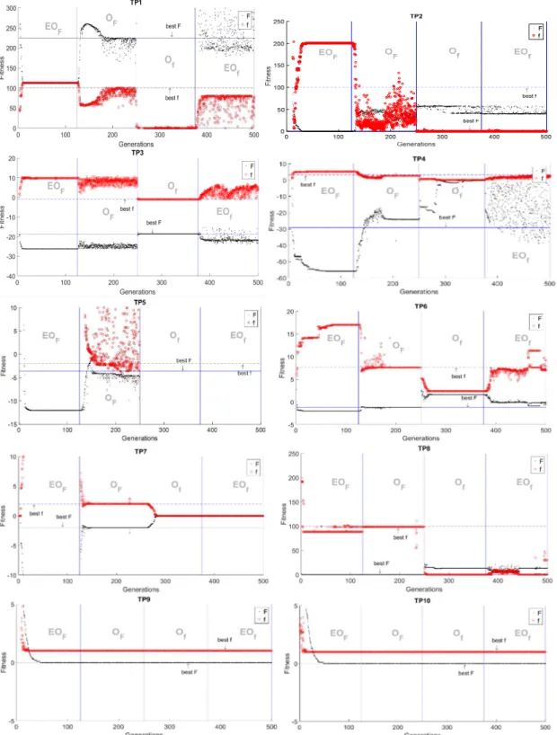
Since BICHEA runs with different convergence strategy in each sector of the total generations, we have plotted fitness landscape of the best five individuals (since the best upper level fitness value fluctuates once better lower level fitness is found) on typical runs for each of the test problems in Fig. 6 to show their impact on different convergence strategies. It can be observed that each strategy is behaving differently for the given benchmark problems to reach towards the known best solution. Optimum solutions close to best known solutions for the problems (TP1 and TP4-TP10) have been obtained in sector 2 i.e. with convergence approach of OF. Notably, the convergence approaches EOF and Of have produced optimum solutions for problems {TP2, TP8-TP10} and
TP3, respectively. We do not have one common convergence strategy that works best for all the problems. All but EOf have
converged to known optimum solution for one or more test problems. It can also be observed that decision makers can have more than one choice of solutions as in TP1 with solution sets of (112.5, 112.5) and (225.0, 100.0) because of bimodal or multimodal nature of the problem. Similarly, (-26.2, 9.8) and (-18.7,-1.0) for TP3 and (0.0, 88.3) and (0.0, 100.0) or even (0.0, 200.0) in some cases for TP8.
We have also done non-parametric Wilcoxon test for ranking (two-tailed) with significance difference of ൏ ͲǤͲͷ for all convergence strategies on every tested problem. The results for fitness values F and f are shown in TABLE VII and TABLE VIII, respectively. The results show that the difference in behavior of the convergence strategies are statistically significant in most of the cases. Especially, the prominent convergence strategies EOF, OF and Ofhave shown the significant difference for fitness F.
Similar results have been obtained for fitness f, however, problems TP9 and TP10, in particular, are not showing significant difference for varying strategies.
All the results discussed above are based on four variations of optimistic convergence strategies. Next, we evaluate performance of pessimistic convergence strategies and compare them with optimistic convergence strategies. TABLE X and TABLE IX compares optimistic and pessimistic approaches for the best and average fitness values obtained over 30 run on each test problem under the same conditions described in TABLE III. Bold values show better (or almost equal) result. Even though the best and average fitness values with pessimistic approaches of almost half of the test problems are matching with optimistic approaches the high variance of best fitness value on 30 runs of pessimistic approach is a concern. Fig. 8 shows the difference of variance οݒܽݎሺܨሻ ൌ ݒܽݎሺܨைሻ െ ݒܽݎሺܨሻ and οݒܽݎሺ݂ሻ ൌ ݒܽݎሺ݂ைሻ െ ݒܽݎሺ݂ሻ where subscripts ܱ and ܲ refer to optimistic and pessimistic
approach respectively. The positive value indicates that the variance of optimistic approach is high and vice versa for negative value. Pessimistic approach has higher variance for all the problem except for TP8 where it has produced a very high variance. Difference of variance of more than േͳ is terminated to േͳ. TP9 and TP10 have a variance value of 0.0.
CROSS EVALUATION MATRIX OF CONVERGENCE STRATEGIES FOR FITNESS ܨ BASED ON WILCOXON RANK TEST ( ൏ ͲǤͲͷ)
Conv. EOF OF Of EOf EOF - TP1-TP7, TP9, TP10 TP1-TP10 TP1-TP10 OF TP1-TP7, TP9, TP10 - TP1-TP8 TP2-TP8 Of TP1-TP10 TP1-TP8 - TP1,TP2, TP4,TP6,TP8 EOf TP1-TP10 TP2-TP8 TP1,TP2, TP4, TP6, TP8 -
CROSS EVALUATION MATRIX OF CONVERGENCE STRATEGIES FOR FITNESS ݂ BASED ON WILCOXON RANK TEST ( ൏ ͲǤͲͷ)
Conv. EOF OF Of EOf EOF - TP1-TP7 TP1-TP8 TP1-TP8 OF TP1-TP7 - TP1-TP8 TP1-TP8 Of TP1-TP8 TP1-TP8 - TP1-TP4, TP6, TP8 EOf TP1-TP8 TP1-TP8 TP1-TP4, TP6, TP8 -
AVERAGE FITNESS COMPARISON OF OPTIMISTIC VS PESSIMISTIC APPROACHES Pessimistic Optimistic Prob F f F f TP1 205.06778 87.70457 224.96290 99.99192 TP2 0.00012 199.99894 0.00012 199.9989 TP3 -18.67884 -1.01559 -18.67862 -1.01533 TP4 -29.06566 4.27437 -29.15966 2.66120 TP5 -3.12431 1.80181 -4.26669 -1.99426 TP6 -1.11267 7.6301 -1.21052 7.61467 TP7 -1.90907 1.90907 -1.96173 1.96173 TP8 0.3518 106.28977 0.36679 92.69204 TP9 0.0000 1.0000 0.00000 1.00000 TP10 0.0000 1.0000 0.00000 1.00000
BEST FITNESS COMPARISON OF OPTIMISTIC VS PESSIMISTIC APPROACHES Pessimistic Optimistic Prob F f F f TP1 223.62584 99.64207 225.00009 99.99968 TP2 0.00002 199.99983 0.00003 199.99971 TP3 -18.6787 -1.01559 -18.67869 -1.01559 TP4 -29.27955 3.55248 -29.19869 3.19633 TP5 -4.28568 -0.32331 -3.67982 -2.01346 TP6 -1.21742 7.62715 -1.20918 7.61450 TP7 -1.9612 1.9612 -1.96001 1.96001 TP8 0.00000 100.00000 0.00000 100.00000 TP9 0.00000 1.00000 0.00000 1.00000 TP10 0.00000 1.00000 0.00000 1.00000
Fig. 8. Comparison of difference of variance for optimistic and pessimistic approaches.
Additionally, the statistical significance of the difference between these two approaches on BICHEA is tabulated in TABLE XI and TABLE XII for fitness ܨ and݂, respectively, with two-tailed Wilcoxon rank test with significance difference of ൏ ͲǤͲͷ. Gens indicate the generation number on which the fitness values are collected for statistical analysis. Major difference is observed between PF and OF where majority of the best fitness values have been obtained as described earlier, however, EPF and EOF, and
Pf and Of did not show any major difference for most of the problems. EPf and EOf show difference in convergence but both are
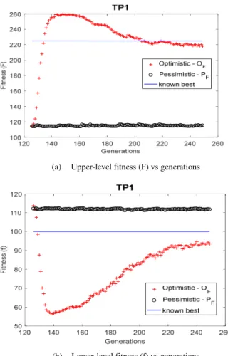
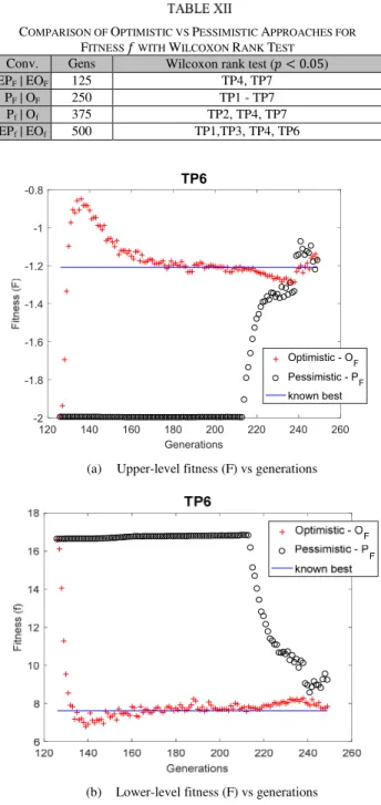
weak convergence techniques as far as attaining close to optimum solution is concerned. We have plotted average fitness of both levels vs generation graph for convergence strategies PF and OF for some of the problems in Fig. 9 and Fig. 10 to show how these
most prominent convergence strategies behave differently on the same problem. The graph of the selected problems TP1 and TP6 shows that PF is generally stuck in local best for most of the generations because of its greedy behavior of selecting the best ݂ value
that gives worst ܨ solution. On the other hand, OF’s greediness towards better ܨ solution leads it towards the known best solution.
For TP1, major difference in fitness ܨ can be observed while in TP6, both strategies eventually converge close to known best, however, they differ a lot in their convergence approaches. OF can also be observed converging faster than PF.
Fig. 9. Plot of average fitness values for problem TP1 w.r.t. optimistic strategy OF and pessimistic strategy PF (a) Upper-level fitness (F) vs generations
Finally, the efficiency of BICHEA can be formulated with the average time complexity of blMutation for ܶ ൌ ʹͲ. It evaluates to ܱሺܰሺʹͲ ൈ ܾ݆ܨݑ݊ܿ ʹͲ݈݃ʹͲሻሻ ൌ ܱሺܰ ൈ ܾ݆ܨݑ݊ܿሻ where N is population size and average sorting time complexity of ݊ sized problem is taken as ݈݊݃݊. Thus the time complexity of overall BICHEA isܱ൫ܩሺʹܾ݆ܰܨݑ݊ܿ ݈ܰ݃ܰ ʹܰሻ൯ ൌ ܱ൫ܰܩሺܾ݆ܨݑ݊ܿ ݈݃ܰሻ൯ where G is the total generation, which can be inversely proportional to ܰ in many general cases for EAs. In that case, the time complexity would be simply ܱሺܾ݆ܨݑ݊ܿ ݈݃ܰሻ or ܱሺܾ݆ܨݑ݊ܿሻ when tested with constant population size ܰ.
COMPARISON OF OPTIMISTIC VS PESSIMISTIC APPROACHES FOR FITNESS ܨ WITH WILCOXON RANK TEST
Conv. Gens Wilcoxon rank test ( ൏ ͲǤͲͷ)
EPF | EOF 125 TP4, TP7
PF | OF 250 TP1 - TP7
Pf | Of 375 TP7, TP8
EPf | EOf 500 TP1, TP2, TP4 - TP6, TP8
COMPARISON OF OPTIMISTIC VS PESSIMISTIC APPROACHES FOR FITNESS ݂ WITH WILCOXON RANK TEST
Conv. Gens Wilcoxon rank test ( ൏ ͲǤͲͷ)
EPF | EOF 125 TP4, TP7
PF | OF 250 TP1 - TP7
Pf | Of 375 TP2, TP4, TP7 EPf | EOf 500 TP1,TP3, TP4, TP6
Fig. 10. Plot of average fitness values for problem TP6 w.r.t. optimistic strategy OF and pessimistic strategy PF (a) Upper-level fitness (F) vs generations
(b) Lower-level fitness (F) vs generations
*HQHUDWLRQV 73 2SWLPLVWLF2) 3HVVLPLVWLF3) NQRZQEHVW
6. CONCLUSION AND FUTURE WORK
Bilevel problem is a class of constraint optimization problem where one of the constraints is an optimization function. Earlier mathematical programming was used to solve these problems, but recently, few partial and complete evolutionary computation approaches have been proposed. Our proposed algorithm BICHEA is a complete evolutionary approach with a single level optimization structure with intermarriage-crossover. It was compared with BLEAQ and Bayesian as partial evolutionary approaches and HPSOBLP as a complete evolutionary approach. BICHEA has outperformed other algorithms in terms of quality of solutions. BICHEA was able to reach towards known global (or near global) optimum solution for all the tested benchmark problems. In this paper, we have realized that different forms of convergence approaches behave differently; however, we have only tested the optimistic approach and its variants. It was demonstrated that our proposed optimistic variants, namely EOF and Of,
have produced global optimal solutions with BICHEA for some of the problems where OF was unable to do so. Future work would
be considered for BICHEA for multi-objective bilevel optimization, which is even a more complex to deal with, as both levels can have multiple objectives to solve. Here, feasibility of any given upper level variable is determined by producing lower level pareto front. Upper level needs to produce the optimal pareto front for the final solution. Some other forms of bilevel problem can be dynamic lower level constraints and discrete search space.
ACKNOWLEDGMENTS
I would like to thank Prof. Grégoire Danoy and Emmanuel Kieffer for providing the data files from their experimental results from [10].
REFERENCES
[1] Y. S. Abu-Mostafa, M. Magdon-Ismail, and H.-T. Lin, Learning From Data. S.l.: AMLBook, 2012.
[2] R. Andreani, V. A. Ramirez, S. Santos, and L. Secchin, Bilevel optimization with a multiobjective problem in the lower level. 2017.
[3] J. Bracken and J. T. McGill, “Mathematical Programs with Optimization Problems in the Constraints,” Operations Research, vol. 21, no. 1, pp. 37–44, 1973.
[4] L. N. de Castro and F. J. Von Zuben, “Learning and optimization using the clonal selection principle,” Evolutionary Computation, IEEE Transactions on, vol. 6, no. 3, pp. 239–251, 2002.
[5] B. Colson, P. Marcotte, and G. Savard, “An overview of bilevel optimization,” Annals of Operations Research, vol. 153, no. 1, pp. 235–256, Sep. 2007.
[6] K. Deb, A. Pratap, S. Agarwal, and T. Meyarivan, “A fast and elitist multiobjective genetic algorithm: NSGA-II,” IEEE Transactions on Evolutionary Computation, vol. 6, no. 2, pp. 182–197, Apr. 2002.
[7] K. Deb and A. Sinha, “Solving Bilevel Multi-Objective Optimization Problems Using Evolutionary Algorithms,” in Evolutionary Multi-Criterion Optimization, M. Ehrgott, C. M. Fonseca, X. Gandibleux, J.-K. Hao, and M. Sevaux, Eds. Springer Berlin Heidelberg, 2009, pp. 110–124. [8] P. Hansen, B. Jaumard, and G. Savard, “New Branch-and-Bound Rules for Linear Bilevel Programming,” SIAM Journal on Scientific and
Statistical Computing, vol. 13, no. 5, pp. 1194–1217, Sep. 1992.
[9] R. G. Jeroslow, “The polynomial hierarchy and a simple model for competitive analysis,” Mathematical Programming, vol. 32, no. 2, pp. 146– 164, Jun. 1985.
[10] E. Kieffer, G. Danoy, P. Bouvry, and A. Nagih, “Bayesian Optimization Approach of General Bi-level Problems,” in Proceedings of the Genetic and Evolutionary Computation Conference Companion, New York, NY, USA, 2017, pp. 1614–1621.
[11] X. Li, P. Tian, and X. Min, “A Hierarchical Particle Swarm Optimization for Solving Bilevel Programming Problems,” in Artificial Intelligence and Soft Computing – ICAISC 2006, 2006, pp. 1169–1178.
[12] H. Liu, Z. Cai, and Y. Wang, “Hybridizing particle swarm optimization with differential evolution for constrained numerical and engineering optimization,” Applied Soft Computing, vol. 10, no. 2, pp. 629–640, Mar. 2010.
[13] P. Marcotte, G. Savard, and D. L. Zhu, “A trust region algorithm for nonlinear bilevel programming,” Operations Research Letters, vol. 29, no. 4, pp. 171–179, Nov. 2001.
[14] R. Mathieu, L. Pittard, and G. Anandalingam, “Genetic algorithm based approach to bi-level linear programming,” RAIRO - Operations Research, vol. 28, no. 1, pp. 1–21, 1994.
[15] Z. Michalewicz and M. Schoenauer, “Evolutionary algorithms for constrained parameter optimization problems,” Evolutionary Computation, vol. 4, no. 1, pp. 1–32, Mar. 1996.
[16] G. Savard and J. Gauvin, “The steepest descent direction for the nonlinear bilevel programming problem,” Operations Research Letters, vol. 15, no. 5, pp. 265–272, Jun. 1994.
[17] A. Sharma, “Analysis of Evolutionary Operators for ICHEA in Solving Constraint Optimization Problems,” presented at the IEEE CEC 2015, Sendai, Japan, 2015, pp. 46–53.
[18] A. Sharma and D. Sharma, “Solving Dynamic Constraint Optimization Problems Using ICHEA,” in Neural Information Processing, vol. 7665, T. Huang, Z. Zeng, C. Li, and C. Leung, Eds. Springer Berlin / Heidelberg, 2012, pp. 434–444.
[19] A. Sharma and D. Sharma, “ICHEA – A Constraint Guided Search for Improving Evolutionary Algorithms,” in Neural Information Processing, vol. 7663, T. Huang, Z. Zeng, C. Li, and C. Leung, Eds. Springer Berlin / Heidelberg, 2012, pp. 269–279.
[20] A. Sharma and D. Sharma, “An Incremental Approach to Solving Dynamic Constraint Satisfaction Problems,” in Neural Information Processing, vol. 7665, T. Huang, Z. Zeng, C. Li, and C. Leung, Eds. Springer Berlin / Heidelberg, 2012, pp. 445–455.
[21] A. Sharma and D. Sharma, “Real-Valued Constraint Optimization with ICHEA,” in Neural Information Processing, vol. 7665, T. Huang, Z. Zeng, C. Li, and C. Leung, Eds. Springer Berlin / Heidelberg, 2012, pp. 406–416.
[22] C. Shi, J. Lu, and G. Zhang, “An Extended Kuhn-Tucker Approach for Linear Bilevel Programming,” Appl. Math. Comput., vol. 162, no. 1, pp. 51–63, Mar. 2005.
[23] A. Sinha and K. Deb, “Bilevel Multi-Objective Optimization and Decision Making,” in Metaheuristics for Bi-level Optimization, Springer, Berlin, Heidelberg, 2013, pp. 247–284.
[24] A. Sinha, Z. Lu, K. Deb, and P. Malo, “Bilevel Optimization based on Iterative Approximation of Multiple Mappings,” arXiv:1702.03394 [math], Feb. 2017.
[26] A. Sinha, P. Malo, and K. Deb, “An improved bilevel evolutionary algorithm based on Quadratic Approximations,” in 2014 IEEE Congress on Evolutionary Computation (CEC), 2014, pp. 1870–1877.
[27] A. Sinha, P. Malo, and K. Deb, “A Review on Bilevel Optimization: From Classical to Evolutionary Approaches and Applications,” IEEE Transactions on Evolutionary Computation, vol. PP, no. 99, pp. 1–1, 2017.
[28] H. von Stackelberg, The Theory of the Market Economy. Oxford University Press, London, 1952.
[29] Stephan Dempe, Foundations of Bilevel Programming, vol. 61. Boston: Kluwer Academic Publishers, 2002.
[30] B. Tessema and G. G. Yen, “A Self Adaptive Penalty Function Based Algorithm for Constrained Optimization,” in IEEE Congress on Evolutionary Computation, 2006. CEC 2006, 2006, pp. 246–253.
[31] L. N. Vicente and P. H. Calamai, “Bilevel and multilevel programming: A bibliography review,” Journal of Global Optimization, vol. 5, no. 3, pp. 291–306, Oct. 1994.
[32] D. J. White and G. Anandalingam, “A penalty function approach for solving bi-level linear programs,” Journal of Global Optimization, vol. 3, no. 4, pp. 397–419, Dec. 1993.
[33] W. Wiesemann, A. Tsoukalas, P.-M. Kleniati, and B. Rustem, “Pessimistic Bilevel Optimization,” SIAM Journal on Optimization, vol. 23, no. 1, pp. 353–380, Jan. 2013.
[34] Y. Zheng, G. Zhang, J. Han, and J. Lu, “Pessimistic Bilevel Optimization Model for Risk-averse Production-distribution Planning,” Inf. Sci., vol. 372, no. C, pp. 677–689, Dec. 2016.