Evaluation of DSR on a Bluetooth Low Energy Network by Simulation

(1)

ASHESI UNIVERSITY COLLEGE

EVALUATION OF DSR ON A BLUETOOTH LOW ENERGY NETWORK BY SIMULATION

APPLIED PROJECT B.Sc. Computer Science

Makafui Fie 2017

ASHESI UNIVERSITY COLLEGE Page | 1

Branding and Identity Guide

The Ashesi brand and logo are integral parts of our worldwide image and identity. We must be careful of how and where the Ashesi is used to ensure we maintain the integrity of our

organization.

This guide has been developed to help you clearly understand our policies towards the use of the Ashesi logo in a variety of mediums, as well as type faces and a color palate to help you produce materials that maintain the brand’s integrity. We would request that you seek approval from the Ashesi University College Marketing Committee before creating any media that reproduces the Ashesi logo.

Declaration

I hereby declare that this Applied Project is the result of my own original work and that no part of it has been presented for another degree in this university or elsewhere.

Candidate’s Signature:

……… Candidate’s Name:

……… Date: ………

I hereby declare that preparation and presentation of this Applied Project were supervised in accordance with the guidelines on supervision of Applied Project laid down by Ashesi University College. Supervisor’s Signature: ……… Supervisor’s Name: ……… Date: ………

(4)

ii

Acknowledgements

I would like to thank my supervisor, Dr Nathan Amanquah, for giving the idea for this project and for his immense direction and supervision.

(5)

iii

Abstract

The Bluetooth Specifications Group recently released a new version of Bluetooth, called Bluetooth Low Energy. It is ideal for battery-powered IoT devices that do not require continuous streaming of information because it is more power efficient and relays information in short bursts, rather than continuously. The asynchronous nature of communication between the Bluetooth Smart nodes introduces a new challenge in terms of routing data among the different nodes. This project developed a simulation tool that simulates how Bluetooth Low Energy creates scatternets among different nodes as well as how routing is achieved. The ability of the routing algorithm to find the shortest route was also tested for and it was shown to be affected by the size of the network.

(6)

iv

Table of Figures

Figure 2.1 Layers of IoT Architecture ... 2

Figure 2.2 Bluetooth stack ... 4

Figure 2.3 Advertising Event ... 6

Figure 2.4 Connection Event ... 6

Figure 2.5 Scatternet Models ... 8

Figure 3.1 Class Diagrams ... 18

Figure 3.2 Structure of Node Module ... 20

Figure 3.3:BLE States ... 21

Figure 3.4:DSR Algorithm ... 24

Figure 3.5 Flow Of simulation ... 25

Figure 3.6 BLE Linear Network with five Nodes ... 26

Figure 3.7 BLE Linear Network with Ten Nodes... 27

Figure 3.8 BLE Linear Network with 20 Nodes ... 27

Figure 3.9 Five-Node Mesh Network ... 28

Figure 3.10 Ten-Node mesh Network ... 28

Figure 4.1 Route discovery time as measured in the different simulations ... 37

(9)

vii

List of Tables

Table 2.1 Technologies of the IoT ... 3

Table 2.2 Routing Protocols in MANETs ... 11

Table 3.1 Destination Node for Each Node in the Five-Node Network ... 29

Table 3.2 Destination node for each node in the Ten-Node Network ... 30

Table 3.3 Destination Nodes for the Twenty-Node Network ... 31

Table 4.1 Summary of Results ... 36

(10)

1

Chapter 1: Introduction

1.1 Background

The Internet of Things (IoT) is an emerging technological trend that continues to increase in popularity, and there is a lot of excitement among both people in technology and the lay man about its potential. IoT is a “collection of many interconnected objects, services, humans and devices that can communicate, share data and information to a common goal in different areas and different applications” (Yousuf, Mahmoud, Aloul, & Zualkernan, 2015). It is often touted as the next big thing to happen in technology because of its potential to make systems more interconnected and efficient. IoT has the ability to transform previously ‘dumb’ devices into intelligent devices that are able to perform daily tasks and coordinate decisions, through evolving technologies such as ubiquitous computing, embedded devices, sensor networks and Internet protocols. IoT is expected to have significant impact in various areas ranging from the personal to enterprise domains, including transportation, healthcare, home automation and service monitoring. (Al-Fuqaha, Guizani, Mohammadi, Aledhari, & Ayyash, 2015)

Some of the wireless interfaces used for communication in IoT devices are Wi-Fi, Bluetooth, ZigBee and 3G (Yousuf, Mahmoud, Aloul, & Zualkernan, 2015). Due to innovations achieved in the development of Bluetooth, it is perceived as having the potential and suitable properties to connect many IoT devices. Bluetooth is an interface that communicates using radio waves over short-range and ad-hoc networks. The Bluetooth Specifications Group recently released a new version of Bluetooth, called Bluetooth Low Energy or Bluetooth Smart. (Bluetooth SIG, 2016) It differs significantly from the older Bluetooth Classic version in terms of the way it works. In addition, it is ideal for battery-powered IoT devices that do not require continuous

(11)

2 streaming of information because it is more power efficient and relays information in short bursts, rather than continuously.

1.2 Research Problem

Scatternets are an integral part of how Bluetooth devices are organized. Bluetooth devices connect with each other to form master to slave networks called piconets. A scatternet is a network formed when a device in one piconet, either a master or slave, joins another piconet and acts as a bridge between the two piconets. Unlike Bluetooth 4.1, Bluetooth smart devices can form scatternets and can act as both piconet masters and slaves, which makes it possible for them to send information over wider areas using multihop routing. (Guo, Harris, Tsaur & Chen, 2015) Routing involves selecting the best paths within the scatternet over which to send data to its destination.

Bluetooth Smart differs significantly from Bluetooth Classic in terms of scatternet formation and scatternet routing. With the specifications for Bluetooth Smart, the procedures used by devices for forming piconets are defined in terms of three roles, namely initiator, scanner and advertiser, (Guo, Harris, Tsaur & Chen, 2015). With Bluetooth Classic, there are three major states, namely standby, connection, and park, while there are nine substates, namely page, page scan, inquiry, inquiry scan, synchronization scan, master response, slave response, and inquiry response. These substates are interim and are used to establish connections and discover devices. (Bluetooth SIG, 2014) Again, communication within Bluetooth Smart networks is asynchronous, meaning that communication between different devices is not timed nor does it happen at the same time.

BLE communication begins when an advertiser sends out a packet to get attention. A client (master) device listens for the adverts and responds with a request when it wants to form a connection. The master device tells the server the hopping sequence of the connection, when to

(12)

3 wake up again so both devices can sleep in between transactions, and if the data channel will be encrypted. (DeCuir, 2014) The asynchronous nature of communication between the Bluetooth Smart nodes introduces a new challenge in terms of routing data among the different nodes.

Because it is a relatively new technology, more work needs to be done in terms of researching and improving on the methods used to form networks among Bluetooth Smart devices and routing data among different nodes. Work has been done in terms of developing algorithms for routing with Bluetooth Classic, but because Bluetooth Smart and Bluetooth Classic work in different ways, new algorithms have to be developed for Bluetooth Smart or the efficacy of existing algorithms need to be evaluated and quantified.

1.3 Project Objectives

 This work develops a simulation tool that simulates how Bluetooth creates scatternets among different nodes as well as how routing is achieved. The simulation will follow the specifications provided by the Bluetooth Specification group that detail the properties of Bluetooth Low Energy.

 Next, it will be used to evaluate the effectiveness of routing algorithms on the Bluetooth Low Energy network.

 The results of this work will include quantifying time bounds for delivering packets within scatternets, which could be used in improving newer versions of Bluetooth Low Energy as well as the current routing algorithms used. With the advent of IoT on the horizon, improving on routing in Bluetooth Low Energy will add to the body of knowledge of Internet of Things and will help to potentially improve the technology.

(13)

4 1.4 Overview of Paper

This chapter introduces the project and the motivation for undertaking this project. Chapter 2 explores research on the key concepts that are associated with this project, namely Internet of Things, Bluetooth, scatternet formation and routing. Chapter 3 describes the methodology employed and gives an overview of the structure of the project and the setups and environments in which simulations were conducted. Chapter 4 presents the results of the simulations and the findings derived from them. Finally, chapter 5 discusses the limitations of the work done and further work that can be done to improve this research.

(14)

1

Chapter 2: Literature Review and Related Works

This presents an overview of literature on the subjects of Internet of Things, Bluetooth and Bluetooth Smart, and routing in Bluetooth.

2.1 Internet of Things

The Internet of Things (IoT) is a “collection of many interconnected objects, services, humans and devices that can communicate, share data and information to a common goal in different areas and different applications” (Yousuf, Mahmoud, Aloul, & Zualkernan, 2015).

2.1.1 Architecture of IoT

The typical architecture for IoT can often be modeled as a 5-layer structure, consisting of the perception, network, middleware, application, and business layers, as shown in Figure 2.1. The perception layer consists of different types of sensors devices that collect and process information, which is then sent to the network layer. Sensor data is obtained over the middleware using various technologies such as RFID, Wi-Fi, ZigBee and Bluetooth Low Energy. The middleware layer has two major responsibilities, which are service management and storing information received from the lower layers in the database. The application layer provides services requested by customers while the business management layer manages the

(15)

2 overall IOT system activities and services. (Al-Fuqaha, Guizani, Mohammadi, Aledhari, & Ayyash, 2015)

Figure 2.1 Layers of IoT Architecture

(Source: Al-Fuqaha, Guizani, Mohammadi, Aledhari, & Ayyash, 2015)

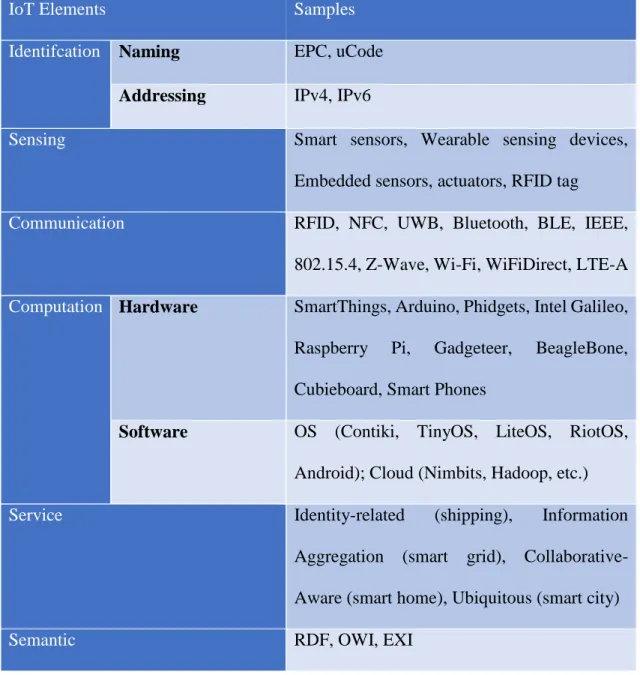
Aside from the layers that make up the IoT architecture, six main elements are needed in order to guarantee the functionality of the IoT. These are identification, sensing, communication, computation, services and semantics. Table 2.1(below) shows these elements and the technologies that are commonly associated with them. This work focuses on the communication logic of IoT devices. With communication, the technologies connect the IoT devices together to enable them communicate with each other to deliver services. Usually, the IoT nodes are expected to operate using low power and in spite of noisy communication links.

(16)

3 Some of the communication protocols used in IoT are Wi-Fi, Z-wave, IEEE 802.15.4 and Bluetooth. Bluetooth is used to exchange data between devices over short ranges.

Table 2.1 Technologies of the IoT

IoT Elements Samples

Identifcation Naming EPC, uCode

Addressing IPv4, IPv6

Sensing Smart sensors, Wearable sensing devices,

Embedded sensors, actuators, RFID tag

Communication RFID, NFC, UWB, Bluetooth, BLE, IEEE,

802.15.4, Z-Wave, Wi-Fi, WiFiDirect, LTE-A

Computation Hardware SmartThings, Arduino, Phidgets, Intel Galileo, Raspberry Pi, Gadgeteer, BeagleBone, Cubieboard, Smart Phones

Software OS (Contiki, TinyOS, LiteOS, RiotOS, Android); Cloud (Nimbits, Hadoop, etc.)

Service Identity-related (shipping), Information

Aggregation (smart grid), Collaborative-Aware (smart home), Ubiquitous (smart city)

Semantic RDF, OWI, EXI

2.2 Bluetooth and Bluetooth Low Energy

Bluetooth is a communication protocol that transmits data over short distances using short-wavelength radio waves (Al-Fuqaha, Guizani, Mohammadi, Aledhari, & Ayyash, 2015).

(17)

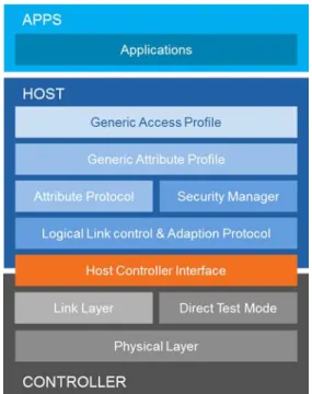
4 Figure 2.2 shows the stack for Bluetooth’s architecture, which consists of three layers. These are the applications layer; the host layer, made up of the Generic Access Profile, the Generic Attribute Profile, the Attribute Protocol and Security Manager, and the Logical Link control and adaptation protocol; and the controller, made up of the link layer, direct test mode and physical layer. A Host Controller Interface serves as an interface between the host and controller layers.

Figure 2.2 Bluetooth stack (Source: Bluetooth SIG, 2014)

Currently there are two main forms of Bluetooth: Basic Rate (BR) and Low Energy (LE). BR has a high-duty cycle while LE has a lower duty cycle with asynchronous communication. Also known as Classic Bluetooth, BR may include an optional Enhanced Data Rate (EDR). The LE system is designed for products that need lower power consumption and lower complexity than BR/EDR.

(18)

5 2.2.1 Bluetooth BR/EDR

The physical layer of the Basic Rate/Enhanced Data Rate operates in the ISM band at 2.4 GHz. It makes use of Time Division Duplex (TDD) frequency hopping channel. Each channel has 1 MHz bandwidth, with adaptive frequency hopping over 79 channels that allows coexistence with Wi-Fi or ZigBee (Decuir, 2014).

2.2.2 Bluetooth Low Energy

Bluetooth Low Energy version 4.0 is touted as being more energy efficient than the classic Bluetooth versions because it transmits data in short bursts, between which it sleeps, while the classic Bluetooth often streams data continuously (Guo, Harris, Tsaur & Chen, 2015). The newest version of BLE is version 4.2. Like Bluetooth BR/EDR, the BLE radio operates on the 2.4 GHz band and has two multiple access schemes, namely Frequency Division Multiple Access (FDMA) and the Time Division Multiple Access (TDMA). With FDMA, there are 40 physical channels separated by 2 MHz, with 37 channels used as data channels and 3 used as advertising channels. With TDMA, one device transmits a packet at predetermined time and a corresponding device responds with a packet after a predetermined interval. (Bluetooth SIG, 2014)

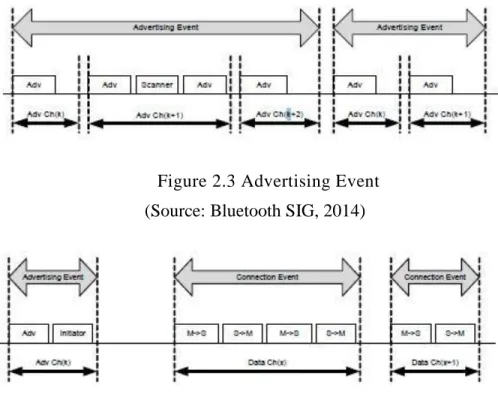
The physical channel has events over which data is transmitted. The two types of events are advertising and connection events. The Link Layer has four states, namely scanning, advertising, initiating and connection (DeCuir, 2014). During an advertising event (shown in Figure 2.3), an advertiser sends out an advertising packet on the dedicated advertising channels, and scanners, which are devices that listen for advertising on the advertising channel without intending to connect, may exchange requests with the advertiser to get more information about it. An initiator device, which is a device that needs to make a connection with another device,

(19)

6 listens in for connectable advertising requests. The advertising event ends and a connection event (shown in Figure 2.4) begins when an advertiser receives a connection request from an initiator. The initiator becomes the master of the piconet while the advertiser becomes the slave. (Bluetooth SIG, 2014) The master provides the hopping sequence for the connection, information on when the slave should wake up again to continue with the connection, and whether the channel will be encrypted (DeCuir, 2014).

Figure 2.3 Advertising Event (Source: Bluetooth SIG, 2014)

Figure 2.4 Connection Event (Source: Bluetooth SIG, 2014) 2.2.3 Scatternet formation in Bluetooth

Communication between Bluetooth devices can occur in two ways. One of the ways is a two-way communication between a master and a slave. The other means is by a slave communicating to another slave through a master. The slave device sends the master a message and this can be forwarded to another device which is a slave of the master. In order for Bluetooth

(20)

7 devices to be able to communicate over a larger area or to pass data between nodes, they form networks called scatternets. A scatternet is made up of two or more piconets. Scatternets are formed when a node in one piconet joins another piconet, thus forming a bridge between the two piconets. Bridge nodes divide their time between piconets by switching between frequency hopping channels and synchronizing to their masters. In Bluetooth Classic, a node can only be a master in one piconet, but can be part of other piconets as a slave. (Persson, Manivannan, & Singhal, 2005)

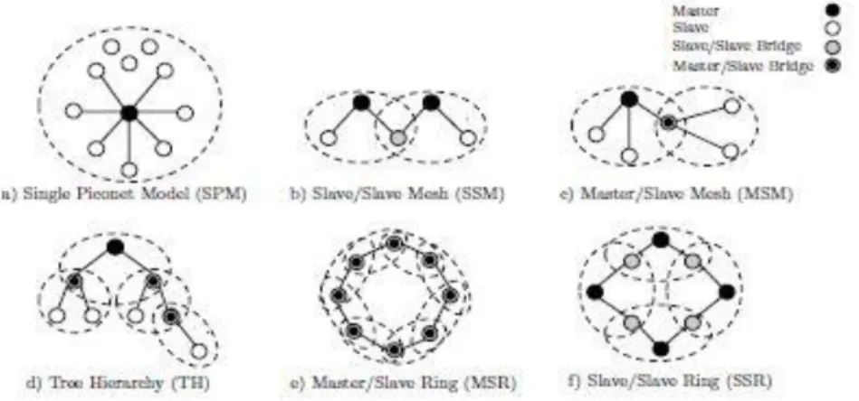
Persson et al (2005) discuss a number of scatternet solutions and their classifications, and these are outlined as follows. There are different categories of scatternets, namely

 Single Piconet Model (SPM),

 Master/Slave Mesh (MSM),

 Slave/Slave Mesh (SSM),

 Three Hierarchy (TH) topology,

 Master/Slave Rings (MSR) and

 Slave/Slave Rings (SSR).

With SPM, a single master and a maximum of seven slaves can communicate, while the rest of the slaves are in PARK mode. The slaves can be substituted if the master needs to communicate with them. MSM connects piconets using a Master/ Slave or Slave/Slave bridges, while SSM scatternets use only Slave/Slave bridges. With TH scatternets, there is a single root node which has descendant tree nodes. MSR and SSR are ring-structured scatternets. Figure 2.5 shows the scatternet models discussed.

(21)

8

Figure 2.5 Scatternet Models (Source: Persson, Manivannan, & Singhal, 2005)

The two main categorizations of scatternet formation are single-hop solutions and multihop solutions. With single-hop solutions, all devices are within radio transmission range of each other. This is also categorized into coordinated and distributed topologies. A master device that is elected to coordinate the scatternet formation forms coordinated topologies. An example of this is Bluetrees, which has different implementations. With Blueroot Grown Bluetree, there is a randomly selected coordinator node called a blueroot, from which a tree is built. Every one-hop neighbor of the master is a slave, and each child is also the master in another piconet. The maximum number of children is 5. Another type of coordinated topology is Bluerings, which makes use of SSR.

With distributed single hop solutions, no single device forms a scatternet. An example is the Tree Scatternet Formation protocol, which forms a TH scatternet. There are free nodes and subtrees that search for other trees to join. When a connection is formed, the master becomes the root, while the slave becomes the leaf node. Root nodes can only connect to other root nodes, with one becoming the master and the other the slave.

(22)

9 With multihop topologies, the devices do not need to be in the same radio transmission range. An example is Distributed Bluetrees, which is similar to Blueroot Grown Bluetree, but has more than one master node, and every neighborhood has a master node that coordinates connections. All the subtrees from the different localities are merged together to form a single tree. Another example is Bluestars, where there is are three phases in the formation of scatternets. Firstly, the devices discover other devices in the neighborhood by exchanging information. They also exchange a weight parameter, which is used to determine the masters of the local neighborhood. The node with the highest weight becomes the master and the ones with lower weights are slaves. The masters then determine other masters in the neighborhood and instruct slaves to form connections with neighboring piconets. The slaves that form the connection become bridge nodes. Finally, there is the SHAPER algorithm, which is based on the Tree Scatternet Formation, but SHAPER allows both root and non-root nodes to form connections. (Persson, Manivannan, & Singhal, 2005)

2.2.3.1 Scatternet Formation in Bluetooth Low Energy

Scatternet formation in BLE differs from that of Bluetooth Classic. This is because Bluetooth Classic limits the number of slaves to a master to seven, while with BLE, there is no limit to the number of slaves that can be connected to a piconet master. Again, BLE has three modes that can be taken up by devices, that are initiator, scanner, or advertiser, which differ from the three major Bluetooth Classic states, namely standby, connection, and park. Initial specifications for Bluetooth Low Energy, with Bluetooth 4.0, made the formation of scatternets impossible. However, the newer Bluetooth 4.1 and 4.2 make scatternet formation possible. In spite of this, not much work has been done so far in terms of developing algorithms for scatternet formation in BLE 4.2. (Guo, Harris, Tsaur & Chen, 2015)

(23)

10 One approach proposed by Guo, Harris, Tsaur and Chen (2015) is an on-demand algorithm for scatternet formation and multihop routing for BLE-based MANETs. This approach involves phases of scatternet formation and route discovery. For scatternet formation, each node has a list , with each master keeping a list of slaves in its piconet, while the slave keps a list of the masters of all its piconets. A new node that enters a network both broadcasts advertisements or scans to listen for advertisements. It may initiate a connection event if it receives an advertisement, and then become a master of a piconet, or it may be connected to by an initiator and become a slave. The next phase is route discovery, where a source node sends a route request packet to its master along with the destination’s information. If the master does not have the destination in its slave list, it starts a breadth-first search by forwarding the request to all its bridge nodes. After receiving responses, it selects the shortest path. This approach was tested on real hardware, specifically, the Broadcom BLE chipset, rather than by means of a simulator.

2.2.4 Routing in Mobile Ad-hoc Networks

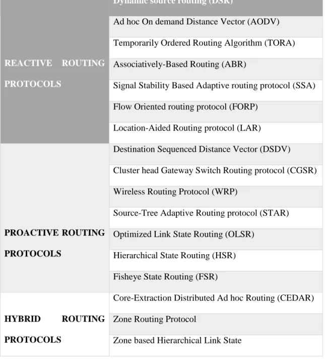
Routing algorithms for mobile ad-hoc networks (MANETs) can be classified into three categories, namely reactive (on-demand), proactive (table-driven) and hybrid routing protocols (Abusalah, Khokhar, & Guizani, 2008). These three categories employ different means of solving the problems of route discovery and route maintenance Table 2.2 displays the categories of routing protocols in MANETs and some examples of routing protocols that can be grouped under the various categories.

(24)

11 Table 2.2 Routing Protocols in MANETs

REACTIVE ROUTING

PROTOCOLS

Dynamic source routing (DSR)

Ad hoc On demand Distance Vector (AODV) Temporarily Ordered Routing Algorithm (TORA) Associatively-Based Routing (ABR)

Signal Stability Based Adaptive routing protocol (SSA) Flow Oriented routing protocol (FORP)

Location-Aided Routing protocol (LAR)

PROACTIVE ROUTING PROTOCOLS

Destination Sequenced Distance Vector (DSDV)

Cluster head Gateway Switch Routing protocol (CGSR) Wireless Routing Protocol (WRP)

Source-Tree Adaptive Routing protocol (STAR) Optimized Link State Routing (OLSR)

Hierarchical State Routing (HSR) Fisheye State Routing (FSR)

HYBRID ROUTING PROTOCOLS

Core-Extraction Distributed Ad hoc Routing (CEDAR) Zone Routing Protocol

Zone based Hierarchical Link State

With proactive algorithms, each node needs to keep information about the entire network. It thus needs to have one or more tables where it keeps the routing information of the

(25)

12 network. This information has to be updated periodically, in case the network’s nature changes. The advantage of this is that the route from a source to a destination is immediately available. However, it consumes more power because of the periodic transmission of updates and may be slow in restructuring due to frequent changes in the network. (Guo, Harris, Tsaur & Chen, 2015) Some examples of proactive algorithms are Destination Sequenced Distance Vector (DSDV) and Optimized Link State Routing (OLSR). With DSDV, each node has a table which contains the shortest path to every other node in the network. The tables are updated and forwarded to other nodes when there is a change in the network. With OLSR, there are two control messages: the hello message and the topology control (TC) message. The hello message is used to discover the nodes within a node’s neighborhood, while TC messages are used to broadcast information periodically on the multipoint relays selected by the node. (Abusalah, Khokhar, & Guizani, 2008)

With reactive algorithms, routes are only established when required by source nodes. This helps to save power and bandwidth because the nodes do not have to periodically send packets containing information on changes to the network nor do they have to maintain and update tables. Nodes have smaller memory requirements as they do not have to maintain routing tables. Again, reactive algorithms do not encounter the challenge of stale routes. However, there is high latency because of the time taken for the establishment of routes from source to destination (Guo, Harris, Tsaur & Chen, 2015) Some examples of reactive protocols are Dynamic Source Routing (DSR) , Ad hoc On demand routing Vector (AODV) and Temporarily Ordered Routing Algorithm (TORA).

To discover routes in DSR, an initiator node transmits a RouteRequest packet which specifies the target node. Each node that receives the packet retransmits the packet until it

(26)

13 reaches the target node. The target node sends back a route reply to the initiator, with a list of the routes taken by the packet. The initiator selects the route with the lowest latency. To maintain routes, when an intermediate node moves away, an error message is sent to the source node by the node adjacent to the broken link. AODV is similar to DSR in terms of sendig a RouteRequest message to the target node, but uses a destination sequence number to determine an up-to-date path to the destination. A node updates its path to a destination only if the destination sequence number of the current packet received is greater than the last number stored at the node. In TORA, routes are defined using a Directional Acyclic Graph, which is rooted at the destination. It uses three control packets: query, update and clear. Query messages are sent to all intermediate nodes until the destination node is reached. An update message is used to update the nodes on the reverse path from destination to source. A clear message is used to clear invalid routes. (Abusalah, Khokhar, & Guizani, 2008)

2.2.4.1 Routing in Bluetooth

To form an ad hoc network, Bluetooth devices form one-hop networks called piconets, and each piconet has one master which connects to a number of slaves. In Bluetooth Classic piconets, a master can connect to a maximum of seven active slaves and two hundred and forty-seven slaves connected in a parked state. A device in one piconet can be a member of another piconet, thus forming a bridge between the two piconets. (Alkhrabash & Elshebani, 2009) 2.3 Simulator Tools for MANETs

In order to evaluate the performance of different routing algorithms on the BLE network, the network will be simulated using a network simulator. The network simulation tools available are either commercial or open source. Some of the more commonly used simulators

(27)

14 for conducting studies in MANETs are Qualnet, GlomoSim, OMNet++, Ns-2, NS-3, OPNET modeler and JIST.

NS-2 is an open-source discrete event simulator. It is dual language, as it makes use of both C++ and OTCL. It can support simulation of routing over wired and wireless networks. Some disadvantages of its usage are its limited and out of date documentation, inability to support more than 500 nodes and the need to recompile every time code is updated. (Manpreet &Malhotra, 2014)

GlomoSim is a public domain simulator that is used for parallel discrete event simulations. It is based on a C-based simulation language called Parsec. GlomoSim is an open source discrete event simulation environment written in C++. One of its strengths is that it can scale to a large number of nodes and it is able to execute simulation in parallel. However, there have been no updates to the software since 2000, after it was migrated to Qualnet, which is a proprietary software. (Chengetania & O’Reilly, 2015)

OPNET (Optimised Network Engineering Tool) is a discrete event, object oriented proprietary network simulation tool. It is able to simulate all types of wired and wireless networks. Its interface is C++, and it has a complete model library and a user-friendly interface. However, it is complex to use and is also expensive because it is a commercial product. (Chengetania & O’Reilly, 2015)

OMNET++ (Objective Modular Network Testbed in C++) is an open source componet based, discrete event simulator tool written in C++. It supports both mobile and wireless networks. It has an easy to use graphical interface, and although not many models are implemented, its architecture is extensible and easy to modify. (Kumar, Kaushik, Sharma, &

(28)

15 Raj, 2012) It also supports large-scale networks and has a vast library for various implementations. (Manpreet &Malhotra, 2014)

NS-2 and OMNET++ are the most widely used simulators for research. Although NS-2 is the most popular simulator for research work, it has a complicated architecture. OMNET++ has a well-designed simulation engine and GUI. (Kumar, Kaushik, Sharma, & Raj, 2012) In view of this, this project will make use of the OMNET++ simulator tool to simulate the Bluetooth Low Energy network.

2.4 Summary of Literature Review and Related Works

This chapter explores the architecture of Internet of Things as well as the technologies associated with it, the Bluetooth and Bluetooth Low Energy technologies and routing in MANETs and Bluetooth. It also discusses scatternet formation in Bluetooth and simulation environments that can be used to simulate the BLE environment. The next chapter describes how the simulation was set up.

(29)

16

Chapter 3: Methodology

This chapter describes the methodology that was used in implementing a Bluetooth Low Energy network and the evaluation of routing algorithms on the network. This project makes use of simulation and experimentation in conducting research on the Bluetooth Low Energy network. Simulation is a preferred means of testing network protocols, because a large network made up of a hundreds of nodes can be tested without needing to set up the physical devices needed to test such a network. This project makes use of the OMNET++ simulation framework to simulate Bluetooth Low Energy version 4.2.

3.1 OMNET++

OMNET++ is a modular discrete event simulation framework which provides the environment for writing simulations for wireless and wired communication networks, as well as other systems. An OMNET++ model is made up of

1. Topology description files 2. Message definitions and 3. Simple modules.

Topology descriptions are written in the NED (Network Environment Description) language, and they describe the module structure. Message definitions are translated into C++ classes while the simple module sources are C++ files. Networks in OMNET++ are made up of simple modules that are written in C++. These simple modules can be grouped into larger modules called compound modules.

In order to simulate a BLE network, there is the need to simulate the formation of a scatternet among Bluetooth nodes. The formation of piconets as well as role switches between

(30)

17 the master and slave roles by the BLE nodes will be simulated. Next, the setup simulates routing in the BLE network by running a routing algorithm on the network and passing data packets between piconets.

The challenge with communication in BLE is the asynchronous nature of communication between BLE nodes. BLE nodes do not communicate directly with each other. Instead, they broadcast messages on dedicated channels to advertise or to form connections with other nodes. The simulation will incorporate these unique characteristics of BLE.

3.2 Routing

Routing on the simulated network is achieved by running a chosen algorithm on the network and passing dummy data packets between a number of piconets. The effectiveness of the algorithm is evaluated by measuring the time taken to pass data from a source node to a destination node. Again, the setup for the simulation is systematically modified to test how changes such as varying the number of nodes as well as the number of piconets affect the network and routing in the network.

3.3 Project Structure

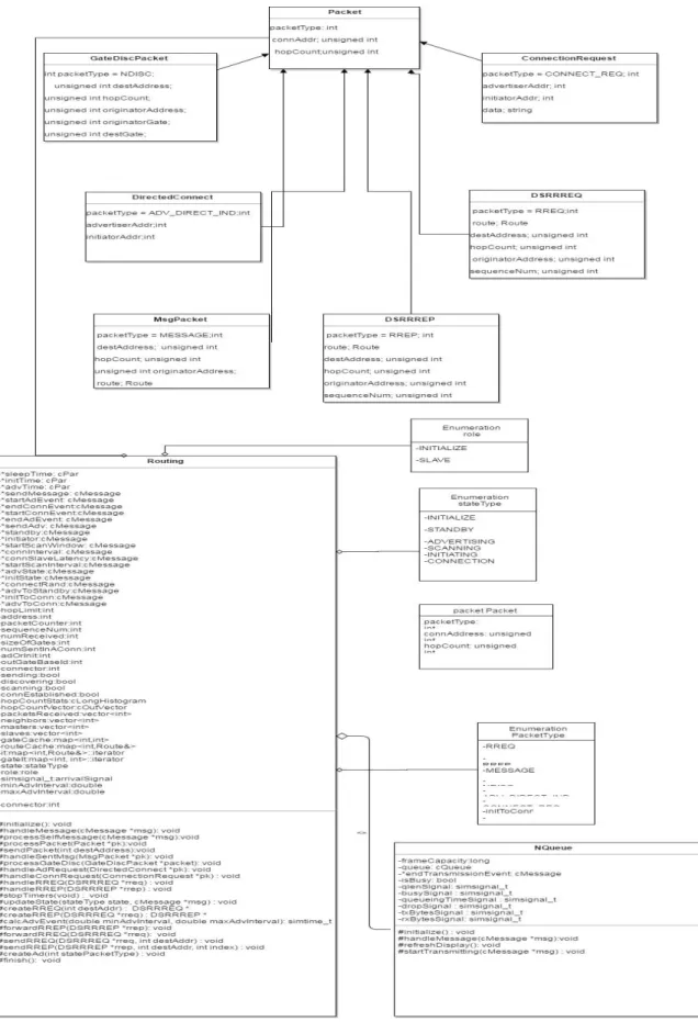
Figure 3.1 shows an overview of the project’s structure including class diagrams for the Routing and NQueue submodules, as well as the message definitions for the packets used in the simulation.

(31)

18 Figure 3.1 Class Diagrams

(32)

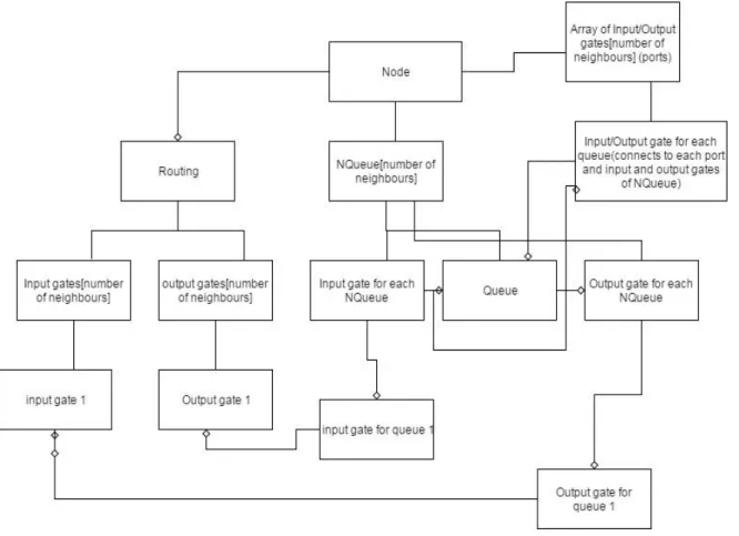
19 A compound module called a Node, whose properties are defined in a Network Description (NED) file, represents each BLE node. The Node consists of two submodules, the Routing and NQueue submodules. The Routing submodule implements most of the logic of the node, including the different states of BLE, discovery of neighboring nodes and routing using the Dynamic Source Routing protocol. The NQueue module implements logic for a queue for messages being sent out and received by the node. A Routing submodule has input and output gates that connect to each queue. There are input and output queues that are connected to each of the node’s neighbors. The structure of each submodule is described in NED files, while the actual implementation is in C++. The network configuration specifies the number of nodes in the network as well as the connections between the different nodes. Appendix B shows the NED definitions for the Node module, and Routing and NQueue submodules. The network configuration is shown in Appendix C, while Appendix D shows a sample of the network descriptions used in setting up the different networks.

(33)

20

Figure 3.2 Structure of Node Module

The simulation makes use of a message implementation called Packet. This is extended to create different types of packets with varying functions. The OMNET++ simulator generates header and C++ files for the Packet implementation, based on the fields provided.

3.3.1 Neighbor Discovery

The structure of the simulation is such that before the start of the simulation, the nodes do not have knowledge about which gates connect to each neighbor. Hence, during the initialization of each node, the node sends a gate discovery message to all its neighbors and attaches the gate id for the specific gate from which the message is sent. The neighbors, upon receiving the message, sends back the message, while specifying the address of the receiving

(34)

21 node and what gate the message is sent on. The initial node sends back the message to the receiving node, which can then extract information on which gate was used to send the message to the originator node. By doing this, each node knows which gate should be used to send information to its neighbors. This information is stored in a cache kept by each node. This procedure is, however, not a feature of BLE and does not affect the core operations of the BLE nodes.

3.4 Implementation of Bluetooth Low Energy

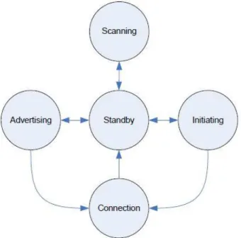
The link layer of Bluetooth Low Energy devices has five states, namely standby, advertising, scanning, initiating, and connection states. Only one state can be active at a time. (Bluetooth SIG, 2014) Figure 3.3 shows the BLE states and the states from which they can be entered.

Figure 3.3:BLE States (Source: Bluetooth SIG, 2014)

(35)

22 For this project, four of the five states, namely standby, advertising, initiating, and connection states, are implemented in OMNET++ by using scheduled messages, which are used as timers and indicate to the node when to transition from one state to another and which state to transition to. This allows the node to transition from one state to another throughout the simulation. The simulation makes use of self-messages, which are messages sent to the node module itself, signaling it to transition from one state to another. During the standby state, the node does not receive or send any messages. From the standby state, the node can transition to the advertising, scanning or initiating states. In the advertising state, the node sends out advertising messages to its neighbors in order to start a connection. These messages may be connectable or non-connectable advertising events, and can receive responses from nodes in the scanning or initiating state. A node in the scanning state listens for undirected scannable advertising messages and can respond with scan requests or responses to get more information about the advertising node. A node in the initiating state listens for directed advertising messages and sends back a connection request in order to start a connection. A node can move to the connection state when it sends or receives a connection request. The receiver of the request becomes a slave while the sender becomes the master of the piconet. (Bluetooth SIG, 2014)

3.5 Implementation of Scatternet Formation

The scatternet formation implemented in this simulation is the master-slave mesh (MSM) where scatternets are formed from piconets that connect using a Master/ Slave or Slave/Slave bridges (Persson, Manivannan, & Singhal, 2005). Either the master or slaves of a piconet can become members of another piconet, hence forming a bridge between the two piconets. This enables the formation of a larger network called a scatternet. Nodes form piconets by sending

(36)

23 or receiving connection requests during an advertising event, and the sender becomes the master of the piconet while the recipient becomes the slave. Nodes form larger networks by connecting through bridge nodes, which may be masters or slaves.

3.6 Implementation of Dynamic Source Routing Algorithm

The Dynamic Source Routing (DSR) algorithm was chosen as the routing protocol to implement within the BLE network. This algorithm is a reactive routing protocol that only begins route discovery for a specific destination when the current node wants to send a message to another node but does not have a route to it in its route cache. The DSR algorithm has the advantage of requiring little memory and uses less energy; hence, it is better suited for BLE devices, which mainly have memory constraints and are battery powered. Figure 3.4 below shows a chart of route discovery in the DSR protocol.

(37)

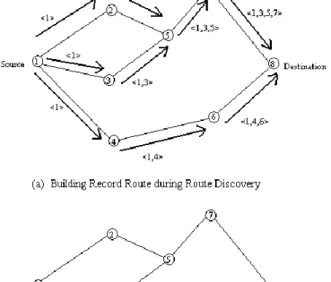
24 Figure 3.4:DSR Algorithm

(Source: Misra, 1999)

For this project, the DSR algorithm was implemented in C++. In this implementation, each node maintains a route cache containing information on the most efficient route to a specified destination point in the network. When a node wants to send a message to another node, it first looks for the destination’s route in the route cache. It sends out a route request to its neighbor nodes if it does not find the route. Neighboring nodes then flood the network with the request until it reaches the destination node. Each intermediate node adds its address to the route before forwarding it to its neighbors. This is demonstrated in diagram (a) of Figure 3.4.

The destination node, upon receiving the route request, sends back a route reply to the source node, with the route from the route request attached, as shown in diagram (b) of Figure

(38)

25 3.4. The destination node only makes use of the route from the first route request to arrive, thus ensuring that the most efficient route, that is the route with the lowest hop count, is obtained. The route reply is sent back using a reversal of the accumulated route information. The source node, upon receiving the route reply, extracts the route and adds it to its cache. It can now send messages using this route. Appendix A shows the implementation for the route discovery process.

Figure 3.5gives a summary of the events that take place during the simulation.

(39)

26 3.7 Simulation Setup

3.7.1 Network Setup for Simulation

In order to analyse the efficiency of the DSR algorithm and how it is affected by the state-based nature of a BLE device, five networks with varied network sizes were set up. Figure 3.6, Figure 3.7, Figure 3.8 and Figure 3.9 (below) show the network set ups that were used in the simulation. Figure 3.6’s and Figure 3.9’s networks have 5 nodes, while Figure 3.7’s and Figure 3.8’s networks have 10 and 20 nodes respectively.

The sizes of the networks make it possible to test how the effectiveness of the routing algorithm is affected by the size of the network. Each successive network setup is double the size of the previous network. For Figure 3.6, Figure 3.7, and Figure 3.8, each node except the first and last have two connections. The linear layout of the setups makes it possible to evaluate the time taken to deliver messages along the possible route. During the simulation, a message is sent from the first node to the last. The hop count of the delivered node is noted, as well as the delivery times of the route request and route reply messages.

(40)

27 Figure 3.7 BLE Linear Network with Ten Nodes

Figure 3.8 BLE Linear Network with 20 Nodes

To test whether the routing algorithm is able to find the most efficient path to a destination node, in this case the route with the least hop count value, two networks were set

(41)

28 up with different possible routes to one destination. During the simulations, messages are sent from Node 0 to Node 4 and Node 9 for the five-node and ten-node networks, respectively. Figure 3.9 and Figure 3.10 show the setups for these networks.

Figure 3.9 Five-Node Mesh Network

(42)

29 3.7.1.1Five-Node Network

3.7.1.1.1 Simulation without traffic

The first simulation for the 5-node network in run for 41.23 seconds, which amounted to t=121.17184679416 seconds in simulated time. In the simulation, Node 0, which is the first node, sends a packet to Node 4, which is the last node, but has to obtain a route first in order to do this. None of the other nodes sends packets, although they connect with each other using advertising and connection requests.

3.7.1.1.2 Simulation with traffic

In the second simulation, Node 0 sends a packet to Node 4. However, with this simulation, the other nodes send packets to each other to generate traffic in the network. Each node sends packets to a specified destination node. Table 3.1 shows the destination nodes for each node. This simulation ran for 1 minute 43.05 seconds in real time, which came to t=241.438523750997 seconds in simulated time.

Table 3.1 Destination Node for Each Node in the Five-Node Network

Source Node Destination Node

Node 0 Node 4 Node 1 Node 3 Node 2 Node 0 Node 3 Node 2 Node 4 Node 1 3.7.1.2Ten-Node Network 3.7.1.2.1 Simulation without traffic

The first simulation for the 10-node network in Figure 3.7 was run for 1 minute and 0.84 seconds, which amounted to t=120.714560110318 seconds in simulated time. The simulation

(43)

30 involved only the first node sending a packet to the tenth node. Again, none of the other nodes sends packets, although they connect with each other using advertising and connection requests. 3.7.1.2.2 Simulation with traffic

In the second simulation, Node 0 sends a packet to Node 9. However, with this simulation, the other nodes send packets to each other to generate traffic in the network. Table 3.2 shows the respective nodes each node sent packets to. This simulation ran for 1 minute and 7.68 seconds in real time, which came to t=120.931436882545 seconds in simulated time.

Table 3.2 Destination node for each node in the Ten-Node Network

Node 0 Node 9 Node 1 Node 5 Node 2 Node 6 Node 3 Node 7 Node 4 Node 8 Node 5 Node 1 Node 6 Node 2 Node 7 Node 3 Node 8 Node 4 Node 9 Node 0 3.7.1.3Twenty-Node Network 3.7.1.3.1 Simulation without traffic

The first simulation for the 20-node network in Figure 3.8 was run for 2 minutes and 36.04 seconds, which amounted to t=105.580188110731 seconds in simulated time. The first node sent packets to the nineteenth node in the network.

3.7.1.3.2 Simulation with traffic

In the second simulation, Node 0 sends packets to Node 19 amidst background traffic, as the other nodes send packets to each other. Table 3.3 shows the destination to which each node

(44)

31 sent packets. This simulation ran for 5 minutes 50.87 seconds in real time, which came to t=105.576720233534 seconds in simulated time.

Table 3.3 Destination Nodes for the Twenty-Node Network

Node 0 Node 19 Node 1 Node 10 Node 2 Node 11 Node 3 Node 12 Node 4 Node 13 Node 5 Node 14 Node 6 Node 15 Node 7 Node 16 Node 8 Node 17 Node 9 Node 18 Node 10 Node 1 Node 11 Node 2 Node 12 Node 3 Node 13 Node 4 Node 14 Node 5 Node 15 Node 6 Node 16 Node 7 Node 17 Node 8 Node 18 Node 9 Node 19 Node 0

3.7.1.4 Networks with different routes to a destination

The simulation for the network set up in Figure 3.9 was run for 2 minutes and 0.50 seconds in real time, which amounted to t= t=135.925661817912 seconds in simulated time. Node 0 tries to send a packet to Node 4. There is more than one possible route to Node 4; hence, the algorithm has to find the most efficient route.

A second simulation was run with the network shown in Figure 3.10 in 4 minutes and 4.81 seconds. This was t=105.560213575405 seconds in simulated time. Node 0 sends a packet

(45)

32 to Node 9, but first has to find the most efficient route. There are multiple routes to Node 9 in the network.

3.7.2 Data Collection

Data was collected on the hop counts of delivered packets, arrival times of route discovery requests at the destination node and route replies at the source node. This data was collected in OMNET++ by emitting the values with pre-registered signals that had been associated with the parameters of data in question. To collect data on the hop counts of delivered packets, a signal for hop count was registered at the beginning of the simulation and was recorded any time a packet was received, along with the hop count for that specific packet. The same was done for the delivery times of packets, but here, the data recorded was derived from finding the difference between the current simulation time and the time at which the packet was created. This was recorded in simtime_t, which is a measure of simulation time.

Routing was simulated on three BLE networks of sizes five, ten and twenty nodes, as described in Section 3.7.2 , in order to find out what effect the size of the network had on the routing algorithm’s efficiency. Routing was also simulated on two networks of sizes five and ten to evaluate whether the algorithm was able to find the best possible route to a destination when presented with more than one possible route. The different networks were run for varying times and under different conditions, and during the simulations, data were collected.

3.7.3 Assumptions of simulation

The simulation was developed under the assumption that the distance between nodes does not affect the success of delivery of packets. It was assumed that once devices are within range, packets sent to them would be delivered correctly. Communication between nodes is

(46)

33 also assumed to be two-way. Again, the costs of all links between nodes are assumed to be equal in value.

The frequency of transmission used by the nodes was not immediately relevant to this simulation, hence was not implemented. Hence, it is assumed that interference does not occur during packet transmission.

In addition, it is assumed that neither do nodes lose their connections to each other nor are packets dropped during transmission. Hence, the simulation does not cater for errors resulting in nodes being lost in the network nor for packets being lost during transmission. Again, nodes are assumed to be stationary.

3.8 Summary of Methodology

This chapter discusses the main elements involved in setting up the simulations for this research. These are the implementation of BLE and its states, routing and the simulation environment. The experiment set-ups used to test the simulation were also described as well as how data was collected and which type of data was collected. The next chapter discusses the results of the experiments and their implications.

(47)

34

Chapter 4: Results and Analysis

After the simulation was set up and the different aspects implemented, data was collected to be analyzed in order to draw conclusions regarding the routing of packets in the BLE network and the factors that may influence the outcome of routing in the network. Due to the asynchronous nature of communication in BLE, it is worthwhile to investigate whether routing can be achieved efficiently.

Various types of data were collected to perform this analysis. These included data about the number of hops and time needed to send a packet from a source node to a destination node. Data about the time taken to find a route was also collected in order to find out how the duration may have been affected by the number of nodes in the network.

4.1 Results

For all simulations run, the connections between the nodes are not predefined. Rather, during the simulation, a node becomes the master or slave of another piconet if it happens to send or receive a connection request from another node, respectively. The formation of connections between nodes is, therefore, randomized.

For the 5-node network, during the simulation (described in Section 3.7.1.1.1), gate discovery ended at t=0.002463348768 seconds. The arrival time for the route request at the destination node was 0.002610112476 seconds in simulated time, while that of the route reply from the destination node to the source node was 0.003188448944 seconds. One packet was sent from Node 0 to Node 4, with a hop count of four. The delivery time of the packet was the same as the delivery time of the route request.

(48)

35 For the simulation (in Section 3.7.1.1.2), the end of the Gate Discovery process occurred at the same time as it did when there was no background traffic in the network. Again, the same value was recorded as for the first simulation for how long it took a route request to be delivered at the destination node, the time taken to deliver a route request, the time taken to deliver a route reply and the time taken for a packet to reach a destination node. One packet was received by Node 4 from Node 0, with a hop count of 4.

For the 10-node network, in the simulation (described in Section 3.7.1.2.1), the gate discovery process ended at t=0.002463348768 seconds. The arrival time for the route request at the destination node was 0.006136427176 seconds in simulated time, while that of the route reply from the destination node to the source node was 0.005159813296 seconds. One packet was received by Node 9 from Node 0, with a hop count value of 9. As with the five-node network, the time taken to deliver a packet was the same as the time taken to deliver a route request.

For the simulation (in Section 3.7.1.2.2), the gate discovery process took the same amount of time to be completed as with the first simulation of the ten-node network. Again, the delivery times for route request, route reply and message packets were the same as for the simulation without traffic generated. One packet was delivered to Node 9 with a hop count of 9.

For the 20-node network, in the simulation (described in Section 3.7.1.3.1), the gate discovery process ended at t=0.002772237137 seconds. The arrival time for the route request at the destination node was 0.0116246039 seconds in simulated time, while that of the route reply from the destination node to the source node was 0.011064804367 seconds. One packet was received by Node 19 from Node 0, with a hop count value of 19. The time taken to deliver a packet was the same as the time taken to deliver a route request.

(49)

36 For the simulation (in Section 3.7.1.3.2), one packet was received by Node 19 from Node 0 with a hop count of 19. The delivery times for route request, route reply and message packets were the same as for the simulation without traffic generated.

Generally, for all the nodes, in the simulations with traffic, the delivery times for route requests had the same value as for message packets, while the delivery time for route replies had a slightly higher value.

Table 4.1 gives a summary of the results described above, while Figure 4.1 and Figure 4.2 visualise the route discovery times and packet delivery times in the three linear networks, in simulations with and without traffic.

Table 4.1 Summary of Results

Simulation Delivery time of route request (in seconds)

Delivery time of route reply (in seconds) Number of packets received by destination Delivery time of message packets (in seconds) Hop count of packet 5-Node Network 0.002610112476 0.003188448944 1 0.002610112476 4 5-Node Network with traffic 0.002610112476 0.003188448944 1 0.002610112476 4 10-Node Network 0.006136427176 0.005159813296 1 0.006136427176 9 10-Node Network with traffic 0.006136427176 0.005159813296 1 0.006136427176 9 20-Node Network 0.0116246039 0.011064804367 1 0.0116246039 19 20-Node Network with traffic 0.0116246039 0.011064804367 1 0.0116246039 19

(50)

37 Figure 4.1 Route discovery time as measured in the different simulations

Figure 4.2 Delivery time of packets as measured in the different simulations

0.005799 0.011296 0.022689 0.005799 0.011296 0.022689 0.000000 0.005000 0.010000 0.015000 0.020000 0.025000

5-Node Network 10-Node Network 20-Node Network

Route Discovery Time (in seconds)

without traffic with traffic

0.002610 0.006136 0.011625 0.002610 0.006136 0.011625 0.000000 0.002000 0.004000 0.006000 0.008000 0.010000 0.012000 0.014000

5-Node Network 10-Node Network 20-Node Network

Delivery time of message packets (in seconds)

(51)

38 In the first simulation described in Section 3.7.1.4, the gate discovery process ended at t=0.002463348768 seconds. The delivery time for the route request and the message packet was 0.001424975132, while that for the route reply was 0.001305782707. One message packet was delivered to Node 4 from Node 0. The hop count recorded was 2, which is the length of the shortest path to Node 4 from Node 0.

In the second simulation with the 10-node network, the gate discovery process ended at t=0.002718544832 seconds. The delivery time for the route request and message packet was 0.001424975132, while that for the route reply was 0.001305782707. One message packet was delivered to Node 9 from Node 0, with a hop count of 3, which was the length of the shortest route to Node 9 in the network.

4.2 Discussion of results

One of the aspects of this research was to determine whether the number of nodes in the network affected the average time taken to deliver packets from a source node to a destination node. Hence, the simulations set up in Sections 3.7.1.1, 3.7.1.2 and 3.7.1.3 explored the effect of network size by using networks that were double the size of the previous network, hence the network sizes of 5, 10 and 20.

Table 4.2 shows the percentage differences in delivery times of route requests, route replies message packets between the 5-node and 10-node networks, and the 10-node and 20-node networks. These values apply to both simulations run with no traffic and simulations run with background traffic, as the values recorded were the same.

(52)

39 Table 4.2 Effect of network size on routing algorithm

% increase in delivery time of route request

% increase in delivery time of route reply % increase in delivery time of message packet 5-node network to 10-node network 135.10% 61.83% 135.10% 10-node network to 20-node network 89.44% 114.44% 89.44%

From the table, it can be observed that there were significant percentage increases for all the values recorded. The most dramatic difference was in the value for the delivery time of a route request at a destination node, which had a percentage increase of 135.10% in the 10-node network from the 5-10-node network. It can therefore be inferred that changes in the network size had a significant effect on the performance of the routing algorithm. This conjecture is based on the fact that the structures of all three networks are similar; all nodes except the first and last node have two connections. Again, the simulations were run under similar conditions, where the first node had to send a route to the last node in the network, hence the node that is farthest away from it. Though the effect of other factors cannot be disregarded, it can be safely concluded that the network size affects the performance of the routing algorithm. It may be difficult to quantify how much of an effect it has, but it can be estimated that doubling the network size may cause an increase of at least 50% in the delivery times of requests and messages.

The generation of traffic did not seem to affect the time of delivery of route requests, route replies and message packets, as the same delivery times were recorded for both when only one node sent a packet and when all nodes in the network sent packets to a designated destination. This can be seen in Table 4.1 where, for instance the same values of

(53)

40 0.002610112476 seconds for route request delivery time and packet delivery time, and 0.003188448944 for route reply delivery time, were recorded for both the simulation of the five-node network without traffic and the simulation with traffic. This may be due to the nature of the OMNET++ simulator, which processes events sequentially and would hence have completed all events that were associated with the message being transmitted, before moving on to the next message. This may not give a realistic depiction of how real devices transmit messages.

From the results of the simulations run in Section 3.7.1.4 to verify the routing algorithm’s effectiveness at finding the most efficient route to a destination node, it is evident that the routing algorithm is able to find the route with the shortest path in terms of hop counts. The algorithm was able to find the shortest path to specified destination node with both simulations, and this was in spite of there being other routes to the same destination, although those routes were longer.

In this implementation of Bluetooth Low Energy, the scatternet formation procedure used is the master-slave mesh, where a master or slave could become a bridge node that connects two piconets. From the results of the simulations ran, described in Section 4.1 above, it can be observed that within the set up networks, nodes were able to connect with each other in master-slave connections, or piconets. These piconets enabled the formation of larger networks or scatternets through bridge nodes. Thus, nodes were able to send messages in a multi-hop manner through the network as they had all connected to form one large network.

(54)

41 4.3 Summary of Results and Analysis

In this chapter, the results obtained from running the simulations of the BLE network have been described and analyzed to arrive at conclusions that meet the objectives of this project as discussed in Section 4.2. The next chapter discusses the conclusions of the project, future work that can be done as well as the limitations of the project.

(55)

42

Chapter 5: Conclusions and Recommendations

5.1 Conclusions

At the conclusion of this project, simulations of BLE networks were successfully built using the OMNET++ simulation environment. The BLE nodes are able to form larger networks and communicate with nodes that are at some distance from them. The DSR algorithm was also implemented in C++ to run on the BLE network simulation. The algorithm is able to discover the shortest route to a destination in the network. It is also able to run on the BLE network and finds a route in spite of the asynchronous nature of the BLE node. This simulation can be built upon and used for further research in the areas of BLE and routing in BLE.

Following the analysis from the previous chapter concerning the number of nodes in the network and whether that has some effect on the efficiency of routing, it can be concluded that the size of the BLE network is directly proportional to the time taken to find a route and deliver packets. This, however, does not affect the algorithm’s ability to find the shortest route.

5.2 Limitations

In its current implementation, BLE is not fully implemented as four out of the five states are implemented, leaving out the scanning state. Again the implementation of the BLE Link Layer is does not include all the properties specified in the Bluetooth Specifications document. These may cause behaviour that differs from an actual BLE device’s characteristics and operations. The current implementation implemented the basic properties of a BLE Link Layer that were necessary to achieve the purposes of this research, but does not consider how the other non-implemented properties may affect the network and routing in the network as it currently is. Particularly, the impact of the scanning state on the simulation needs to be explored.

(56)

43 Again, this implementation analyzed one routing algorithm, which is a type of reactive routing protocols. It may, therefore not accurately represent how efficient routing achieved by other routing protocols or types of routing protocols, including proactive protocols, would be. The frequency selection process was also not implemented, therefore its possible effects on the simulation could not be quantified.

5.3 Future Work

Subsequent to the limitations above, future work may involve implementing all the states of the BLE node and as many properties of the BLE architecture that may affect the node’s performance or operations. Other scatternet formation types can also be implemented and evaluated which is more effective for the BLE network. More routing algorithms, especially those that are examples of the other types of routing protocols can be implemented and evaluated to determine which among them is better suited for this network. Future implementations can also include an implementation of frequency hopping and channel selection of the BLE node. Studies can be conducted on how these affect the efficiency of routing, and how they may or may not affect the structure of routing.

(57)

44

References

Abusalah, L., Khokhar, A., & Guizani, M. (2008). A survey of secure mobile Ad Hoc routing protocols. IEEE Communications Surveys & Tutorials, 10(4), 78-93.

http://dx.doi.org/10.1109/surv.2008.080405.

Al-Fuqaha, A., Guizani, M., Mohammadi, M., Aledhari, M., & Ayyash, M. (2015). Internet of Things: A Survey on Enabling Technologies, Protocols, and Applications. IEEE

Communications Surveys & Tutorials, 17(4), 2347-2376. http://dx.doi.org/10.1109/comst.2015.2444095.

Alkhrabash, A.-A. S., & Elshebani, M. (2009). Routing Schemes for Bluetooth Scatternet Applicable to Mobile Ad-hoc Networks. 9th International Conference on

Telecommunication in Modern Satellite, Cable, and Broadcasting Services, 2009 (pp. 560 -563). IEEE Conference Publications.

Bluetooth SIG. (2014). Specification of the Bluetooth System Version 4.2: Architecture. Bluetooth SIG. (Vol. 1), 171 – 174.

Bluetooth SIG. (2014). Specification of the Bluetooth System Version 4.2: Core System Package [Low Energy Controller Volume]. Bluetooth SIG. (Vol. 6), 30 – 31. Bluetooth SIG. (2014). Specification of the Bluetooth System Version 4.2: Core System

Package [BR/EDR Controller Volume]. Bluetooth SIG. (Vol. 2), 159. Bluetooth SIG. (2016). Bluetooth core specification. Retrieved from

https://www.bluetooth.com/specifications/bluetooth-core-specification.

Chengetania, G. & O’Reilly, G. B. (2015). Survey on simulation tools for wireless mobile ad hoc networks. 2015 IEEE International Conference on Electrical, Computer and Communication Technologies. (pp. 1-7). IEEE Conference Publications.

(58)

45 DeCuir, J. (2014). Introducing Bluetooth Smart: Part 1: A look at both classic and new

technologies. IEEE Consumer Electronics Magazine, 3(1), 12-18. http://dx.doi.org/10.1109/mce.2013.2284932

Guo, Z., Harris, I. G., Tsaur, L.-F., & Chen, X. (2015). An On-demand Scatternet Formation and Multi-hop Routing Protocol for BLE-based wireless Sensor Networks. I2015 IEEE Wireless Communications and Networking Conference (WCNC) (pp. 1590 - 1595). IEEE Conference Publications.

Kumar, A., Kaushik, S. K., Sharma, R., & Raj, P. (2012). Simulators for Wireless Networks: A Comparative Study. 2012 International Conference on Computing Sciences (pp. 338-342). IEEE Conference Publications.

Manpreet, &Malhotra, J. (2014). A Survey on MANET Simulation Tools. 2014 International Conference on Innovative Applications of Computational Intelligence on Power, Energy and Controls with their Impact on Humanity. (pp. 495-498). IEEE Conference Publications.

Mishra P. (1999). Routing Protocols for Ad Hoc Mobile Wireless Networks. Retrieved from http://www.cse.wustl.edu/~jain/cis788-99/ftp/adhoc_routing/.

Persson, K., Manivannan, D., & Singhal, M. (2005). Bluetooth scatternets formation: Criteria, models and classification. Ad Hoc Networks, 3(6), 777-794.

http://dx.doi.org/10.1016/j.adhoc.2004.03.014.

Yousuf, T., Mahmoud, R., Aloul, F., & Zualkernan, I. (2015). Internet of Things (IoT) Security: Current status, challenges and countermeasures. International Journal For Information Security Research, 5(4), 608-616.