Working paper
2019-07
Statistics and EconometricsISSN 2387-0303
Quantile regression: a penalization approach
ÈOYDUR0pQGH]&LYLHWD0&DUPHQ$JXLOHUD0RULOOR5RVD(/LOOR
Serie disponible en http://hdl.handle.net/10016/12
Creative Commons Reconocimiento-NoComercial- SinObraDerivada 3.0 España (CC BY-NC-ND 3.0 ES)
Quantile regression: a penalization
approach
Álvaro Méndez Civieta∗ † M. Carmen Aguilera-Morillo∗ † Rosa E. Lillo∗ †
May 28, 2019
Abstract
Sparse group LASSO (SGL) is a penalization technique used in re-gression problems where the covariates have a natural grouped struc-ture and provides solutions that are both between and within group sparse. In this paper the SGL is introduced to the quantile regres-sion (QR) framework, and a more flexible verregres-sion, the adaptive sparse group LASSO (ASGL), is proposed. This proposal adds weights to the penalization improving prediction accuracy. Usually, adaptive weights are taken as a function of the original non-penalized solution model. This approach is only feasible in then > p framework. In this work, a solution that allows using adaptive weights in high-dimensional sce-narios is proposed. The benefits of this proposal are studied both in synthetic and real datasets.
keywords: quantile regression; group variable selection; adaptive sparse
group LASSO; high dimension; weight calculation
1
Introduction
Along years, regression has become a key method in statistics. Ordinary least squares (OLS) regression estimates the conditional mean response of a variable as a function of the covariates. However, OLS estimators relies on certain hypothesis over the first two moments that are not always verified in practical applications. Ever since the seminal work of [Koenker and Bassett,
∗
Department of Statistics, University Carlos III of Madrid. †
1978], quantile regression (QR) models have gained importance when dealing with this kind of situations. QR models allow a relaxation of the classical first two moment conditions over the model error, and it offers robust estima-tors capable of dealing with heteroscedasticity and outliers. QR models can also estimate different quantile levels of a response variable, giving a precise insight of the relation between response and covariates at upper and lower tails. This can provide a much richer point of view than OLS regression. For a full review on quantile regression, we recommend [Koenker, 2005].
In recent years, high-dimensional data in which the number of covari-ates p is larger than the number of observations n (p n), has become increasingly common. This problem can be found in many different areas like computer vision and pattern recognition [Wright et al., 2010], climate data over different land regions [Chatterjee et al., 2011], and prediction of cancer recurrence based on patients genetic information [Simon et al., 2013]. In these scenarios, variable selection gains special importance offering sparse modeling alternatives that help identifying significant covariates and enhancing prediction accuracy. One of the first and more popular sparse regularization alternatives is LASSO, which was proposed by [Tibshirani, 1996] and adapted to the QR framework by [Li and Zhu, 2008], that devel-oped the piece-wise linear solution of this technique. LASSO is a technique that penalizes each variable individually, enhancing thus individual sparsity. However, in many real applications variables are structured into groups, and group sparsity rather than individual sparsity is desired. One can think for example in a genetic dataset grouped into gene pathways. This prob-lem was faced by the group LASSO penalization of [Yuan and Lin, 2006], and opened the doors to more complex penalizations like the sparse group LASSO [Friedman et al., 2010], which is a linear combination of LASSO and group LASSO providing solutions that are both between and within group sparse. With the same objective in mind, [Zhou and Zhu, 2010] proposed a hierarchical LASSO. To the best of our knowledge, the SGL technique has not been studied in the framework of QR models, so this gap is addressed first, extending the SGL penalization to quantile regression.
[Zou, 2006] was the first to propose the usage of specific weights for each variable on LASSO penalization as a way to increase the model flexibility. This idea, generally known as the adaptive idea, was then extended to other penalizations. The weights of the adaptive idea are typically defined in the
literature based on the results of non-penalized models. This definition is a key step for the demonstration of the oracle properties of the estimators [Fan and Li, 2001], but it is restrictive in the sense that limits the usage of adap-tive penalizations just to the case in which solving a non-penalized model is a feasible first step. This approach, focused on the oracle properties under low-dimensional scenarios is observed in [Nardi and Rinaldo, 2008] for the adaptive group lasso, [Ciuperca, 2019] for the adaptive group LASSO and the adaptive fused LASSO [Ciuperca, 2017] in QR, [Wu and Liu, 2009] for the adaptive LASSO and scad penalizations in QR, and [Zhao et al., 2014] for an adaptive hierarchical LASSO in QR regression among others. It is inter-esting to remark especially the work developed in [Poignard, 2018], in which an adaptive sparse group LASSO estimator suitable for low-dimensional sce-narios (with n>p) is proposed, studying its theoretical properties for a set of general convex loss functions.
The main contribution of this work lies here. An adaptive sparse group lasso (ASGL) for quantile regression estimator is defined, working specially on enabling the usage of the ASGL estimator in high-dimensional scenarios (with p n). In order to achieve this objective, four alternatives for the weight calculation are proposed. It is worth noting that these weight calcu-lation alternatives can be used no only in the case of the ASGL estimator, but also in the rest of the adaptive-based estimators available in the liter-ature. The performance of this alternatives is also studied in the case of low-dimensional scenarios, making the proposed work a good alternative for both high-dimensional and low-dimensional problems.
The rest of the paper is organized as follows. In Section 2 some basic theoretical concepts are introduced, along with the formal definition of the sparse group LASSO in quantile regression. This definition is extended to the adaptive idea in Section 3, proposing the ASGL estimator. Section 4 introduces the weights calculation alternatives for high-dimensional scenar-ios. Section 5 shows the advantages of this proposal in different synthetic datasets in high and low-dimensional scenarios. In Section 6 the proposed model is used in a real dataset, a genomic dataset including gene expression data of rat eye disease first shown in [Scheetz et al., 2006]. The computa-tional aspects of the problem are briefly commented on Section 7, and the conclusions are provided in Section 8.
2
Penalized quantile regression
Consider a sample ofnobservations structured as D= (yi,xi), i= 1, . . . , n
from some unknown population and define the following linear model, yi =xtiβ+i, i= 1, . . . , n (1)
whereyi is the i-th observation of the response variable, xi ≡(xi1, . . . , xip)
is the vector ofp covariates for observation iandi is the error term.
Let us introduce now the quantile regression framework by defining the loss check function,
ρτ(u) =u(τ−I(u <0)) (2)
where I(·) is the indicator function. In their seminal work [Koenker and Bassett, 1978] proved that theτ-th quantile of the response variable can be estimated by solving the following optimization problem,
˜ β= arg min β∈Rp ( 1 n n X i=1 ρτ(yi−xtiβ) ) . (3)
Quantile regression models allow a relaxation of the classical first two mo-ment conditions over the model error, and it offers robust estimators capable of dealing with heteroscedasticity and outliers.
We call high-dimensional scenarios to the datasets in which p is much larger than n (p n). This problem is becoming more and more common nowadays, and can be observed in many different fields of research such as computer vision and pattern recognition [Wright et al., 2010], climate data over different land regions [Chatterjee et al., 2011] or prediction of cancer recurrence based on patients genetic information [Simon et al., 2013]. An alternative that has been intensively studied in recent years for dealing with these scenarios is the penalization approach. By penalizing a regression model it is possible to perform variable selection and improve the accuracy and interpretability of the models. Since it is a continuous process, it also offers more stable solutions than other alternatives.
One of the best known variable selection penalization methods is the least absolute selection and shrinkage operator, generally known as LASSO, pro-posed initially by [Tibshirani, 1996] which, in the case of the QR framework solves, ˆ β(λ) = arg min β∈Rp ( 1 n n X i=1 ρτ(yi−xtiβ) +λkβk1 ) , (4)
whereρτ(·) is the QR check function defined in (2). The LASSO
penaliza-tion sends many β components to zero, offering sparse solutions and per-forming automatic variable selection. In the last years, many LASSO-based algorithms have been proposed. [Yuan and Lin, 2006] introduced the group LASSO penalization as an answer for the need to select variables not individ-ually but at the group level. This penalization solves the following problem,
ˆ β(λ) = arg min β∈Rp ( 1 n n X i=1 ρτ(yi−xtiβ) +λ K X l=1 √ pl β l 2 ) , (5)
whereK is the number of groups, βl ∈
Rpl are vectors of components ofβ from the l-th group, and pl is the size of the l-th group. The group LASSO
penalization performs in a similar way to LASSO, but while LASSO enhances sparsity at individual level, group LASSO enhances sparsity at group level, selecting, or sending to zero whole groups of variables.
Initially proposed by [Friedman et al., 2010], the sparse group LASSO (SGL) is a linear combination of LASSO and group LASSO penalizations. Well known in linear regression and other GLM models, to the best of our knowledge SGL has not been adapted to QR, and as a first step in the paper, this penalization is introduced in the framework.
ˆ β= arg min β∈Rp ( 1 n n X i=1 ρτ(yi−xtiβ) +αλkβk1+ (1−α)λ K X l=1 √ pl β l 2 ) . (6) As in LASSO and group LASSO, SGL solutions are, in general, sparse, send-ing many of the predictor coefficients to zero. However, while LASSO solu-tions are sparse at individual level, and group LASSO solusolu-tions are sparse at group level, SGL offers both between and within group sparsity, outper-forming both alternatives.
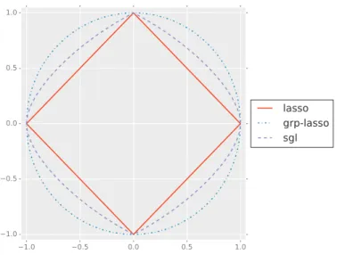
From an optimization perspective, equation (6) defines a sum of con-vex functions. This concon-vexity ensures that the solution of the minimization problem is a global minimum. Figure 1 shows the constrains defined by LASSO, group LASSO and SGL in the case of a single 2-dimensional group of predictors.
3
Adaptive sparse group LASSO
Variable penalization in SGL is somehow restrictive in the sense that it penalizes equally all the variables in LASSO part (giving them the same
Figure 1: Contour lines for LASSO, group-LASSO and sparse-group-LASSO penalties in the case of a single 2-dimensional group
importance), and it penalizes only based on the group size in the group LASSO part. The usage of the adaptive idea, initially introduced by [Zou, 2006], is proposed here as a way to solve this limitations. In this work, a variant of the SGL penalization, the adaptive sparse group LASSO (ASGL) for quantile regression is defined. The ASGL estimator for QR is the result of the following minimization process,
ˆ β= arg min β∈Rp ⎧ ⎨ ⎩ 1 n n i=1 ρτ(yi−xtiβi) +αλ p j=1 ˜ wj|βj|+ (1−α)λ K l=1 √ plv˜lβl 2 ⎫ ⎬ ⎭, (7) wherew˜ ∈Rp andv˜∈RK are known weights vectors. The intuition behind these weights is that if a variable (or group of variables) is important, it should have a small weight, and this way would be lightly penalized. On the other hand, if it is not important, by setting a large weight it is heav-ily penalized. This enhances the model flexibility and improves prediction accuracy. It is worth saying that this formulation defines a convex function and thus, the global minimum can be found.
The adaptive idea has been used in many LASSO-based formulations in recent years. One can see for instance [Wu and Liu, 2009] that introduces the adaptive LASSO in quantile regression, [Ciuperca, 2017] where an adap-tive fused group LASSO is defined, or [Zhao et al., 2014] that proposes an
adaptive hierarchical LASSO among others. When dealing with an adap-tive estimator, the general tendency found in the literature is to study the so-called oracle properties of the estimator, defined initially in [Fan and Li, 2001]. One estimator is oracle if it is (asymptotically) normally distributed and recovers the true underlying sparse model.
A major drawback of this approach in our opinion is precisely that it is focused on the asymptotic behavior of the estimators, when the num-ber of observations n diverges, or in the double-asymptotic behavior, when the number of parameters p diverges with the number of observations n. However, it does not consider the case of high-dimensional scenarios, where p n. A typical step in the demonstration of the oracle behavior of the estimators is to define the adaptive weights based on the result of the unpe-nalized model,
˜
w= 1
|β˜|γ, (8)
where |·|denotes the absolute value function, γ is a non negative constant andβ˜is the solution vector obtained from the unpenalized model (described, in the case of the QR framework, in equation (3)). This approach makes un-feasible the usage of adaptive models in high-dimensional scenarios in which solving unpenalized models is not a realistic approach. The work developed by [Poignard, 2018] is of special interest. Here an adaptive sparse group lasso estimator is defined in a general set of convex functions. However, the author is centered on studying the asymptotic behavior of the estimator, and thus, its usage in real applications is restricted to low-dimensional scenarios. The proposal developed in this work, on the other hand, can be used both in high-dimensional and low-dimensional scenarios.
4
Adaptive weights calculation
The objective of this section is to introduce different alternatives for the calculation of weights in the adaptive framework. The intuitive idea is to find a way to substitute β˜, the solution from the unpenalized model, un-feasible in high-dimensional scenarios, in the calculation of the adaptive weights. This problem will be faced making use of two dimensionality re-duction techniques, principal component analysis (PCA) and partial least squares (PLS). The proposed weight calculation alternatives can be used both in high-dimensional and low-dimensional scenarios. It is worth
remark-ing that these alternatives can be applied not only to the ASGL algorithm, but also to other adaptive-based algorithms.
4.1 Principal components analysis
Given the covariates matrix X ∈ Rn×p defined in equation (1), with
max-imum rank r = min{n, p}, consider the matrix of principal components Q∈Rp×r defined in a way such that the first principal component has the
largest possible variance, and each succeeding component has the largest possible variance under the constraint that it is orthogonal to the preceding components. From an algebra perspective, the principal components in Q define an orthogonal change of basis matrix that maximize the variance ex-plained from X. Consider Z =XQ ∈ Rn×r the projection of X into the
principal components subspace. Two weight calculation alternatives based on principal components are proposed.
4.1.1 Based on a subset of components
Consider the sub-matrixQd= [q1, . . . ,qd]twhereqi∈Rp is the i-th column
of the matrixQ, andd∈ {1, . . . , r}is the number of components chosen. Let αpca,d ∈ [0,100] be the percentage of variability from X that the principal
components inQdare able to explain. Ifd=rthen the principal components
inQdare able to explain all the original variability fromX, andαpca,d= 100,
if d < r then αpca,d < 100. The number of components chosen in order to
explain up to a certain percentage of variability is fixed by the researcher. ObtainZd=XQd∈Rn×dthe projection ofX into the subspace generated
byQdand solve the unpenalized model,
˜ β= arg min β∈Rp ( 1 n n X i=1 ρτ(yi−zitβ) ) . (9)
This model defines a low-dimensional scenario whereβ˜∈Rd. Using this
so-lution, it is possible to obtain an estimation of the high-dimensional scenario solution,βˆ=Qdβ˜∈Rp. Finally, the weights are estimated as,
˜ wj = 1 |βˆj|γ1 and v˜l= 1 ˆ βl γ2 2 , (10)
whereβˆj is the j-th component fromβ,ˆ βˆl is the vector of components ofβ
from the l-th group, andγ1 andγ2 are non negative constants usually taken in[0,2].
4.1.2 Based on the first component
A more straightforward approach based on the first principal component is also proposed. The principal components are no more than lineal combi-nations of the original variables. Therefore, the first principal component q1 ∈Rp, which is the first column of the matrixQ, includes one weight for
each of the p original variables. This proposal consists of calculating the weights as, ˜ wj = 1 |q1j|γ1 and v˜l= 1 q1l γ2 2 , (11)
where q1j is the j-th component from q1 and defines the weight associated
to the j-th original variable, ql1 is the vector of components of q1 from the l-th group and γ1 andγ2 are non negative constants usually taken in[0,2].
4.2 Partial least squares
The principal components are defined in a way such that they capture the maximum possible variance from X under the constraint that they are or-thogonal to the rest of the principal components. However, being relevant for describing the variance of X does not necessarily mean that a principal component is relevant for predicting the value of y. Partial least squares (PLS) is a dimensionality reduction technique centered on maximizing the covariance betweenX and y.
Given the covariates matrix X ∈ Rn×p defined in equation (1), with
maximum rank r = min{n, p}, consider the matrix of PLS components T ∈Rp×s and the projection ofX into the subspace generated by T: U =
XT ∈ Rn×s. The matrix of PLS components T defines a non-orthogonal
change of basis matrix whose projectionUis computed in a way such that the first projection vector, u1 ∈ Rn has the largest possible covariance with y,
and each succeeding projection vector has the largest possible covariance with y under the constraint that it is uncorrelated to the rest of the projection vectors.
Given the sub-matrixTd= [t1, . . . ,td]twhere ti ∈Rp is the i-th column
of the matrix T, and d ∈ {1, . . . , s} is the number of components chosen, let αpls,d ∈ [0,100] be the percentage of variability from X that the PLS
components in Td are able to explain. The non-orthogonality of T implies
than the rank of X, s ≤r, and then the maximum possible percentage of variability explained by the PLS componentsαpls,s is lower than 100%.
In the case of principal components analysis, the matrix of principal componentsQdefines an orthogonal change of basis matrix that results into an orthogonal projection matrix Z maximizing the variance of X. On the other hand, PLS defines a non-necesarily orthogonal change of basis matrix T that results into an uncorrelated projection matrix U maximizing the covariance between U and y. Similarly to the alternatives proposed for PCA, two alternatives of weight calculation using PLS are proposed: based on a subset of PLS components, and based just on the first PLS component.
5
Simulation studies
This section shows the performance of the proposed ASGL model under different synthetic dataset examples. Given that the ASGL formulation in equation (7) includes a weight penalization on the group LASSO part based on the group size (the term √pl), two model formulations are considered:
• Adaptive LASSO in sparse group LASSO (AL-SGL), wherew˜ 6=1but
˜
v=1, in which the adaptive idea is only applied to the LASSO part.
• Adaptive sparse group LASSO (ASGL), wherew˜ 6=1and v˜6=1. Furthermore, the four weight calculation alternatives proposed are studied:
• PCA weights based on regression on a subset of principal components, we denote this aspcad;
• PCA weights based on the first principal component, we denote this aspca1;
• PLS weights based on regression on a subset of PLS components, we denote this asplsd;
• PLS weights based on the first PLS component, we denote this aspls1. The total number of componentsdused in the weight estimation inplsd
and pcad is chosen such that in both cases the percentage of variability
ex-plained from the original matrix X is αpca,d = 80%, αpls,d = 80%. As
commented along Section 4, due to the non orthogonality of the PLS com-ponents it is possible for the maximum possible variability explained by the
PLS components αpls,s to be smaller than 80%. In these cases we consider
dsuch thatαpls,d =αpls,s.
The results obtained by the models proposed in this work are compared with the results from LASSO and SGL formulations. For each dataset D,
a partition into three disjoint subsets, Dtrain, Dval and Dtest is considered.
Dtrain is used for training the models, this is, solving the model equations. Dval is used for validation, this is, optimizing the model parameters. This
optimization is performed based on grid-search. Finally, Dtest is used for testing the models prediction accuracy. The model parameters are optimized based on the minimization of the quantile error, defined as,
Ev = 1 #Dval X (yi,xi)∈Dval ρτ(yi−xtiβˆ), (12)
whereρτ(·) denotes the quantile function defined at (2), and#denotes the
cardinal of a set. The final model error is calculated overDtest as, Et= 1 #Dtest X (yi,xi)∈Dtest ρτ(yi−xtiβˆ). (13)
Additionally, the following metrics for evaluating the performance of the methods are considered:
• ˆ β−β 2
the euclidean distance between the estimated vector and the true vector;
• true positive rate (TPR)=P( ˆβi 6= 0|βi6= 0);
• true negative rate (TNR)=P( ˆβi = 0|βi = 0);
• correct selection rate (CSR)=P( ˆβ =β).
In these simulations we consider τ = 0.5. Each simulation example has been executed 50 times considering 100/100/5000observations in the train / validate / test samples. The results have been summarized in terms of the mean and standard deviation values, and the best result from each metric is highlighted.
The general simulation scheme comes from the model, y =Xβ+, ∼t(3),
whereX is generated from a standard Gaussian distribution. Variables are organized in groups, and within group correlation of 0.5 and 0 otherwise
is considered. The scheme used here is an adaptation of other simulation schemes used in [Wu and Liu, 2009] and [Zhao et al., 2014].
We are interested on studying the performance of the proposed models under different situations, for this reason three main scenarios are defined, the first two are high-dimensional and the third one is low-dimensional. The scenario from Section 5.1 is a high-dimensional scenario that considers a sparse distribution of the significant variables along many groups, the sce-nario from Section 5.2 is a high-dimensional scesce-nario that considers a dense distribution of the significant variables in a few number of groups. It is in-teresting to test the performance of the models as the number of variables increase. For this reason, two cases are considered in each of these two sce-narios. A dataset having225variables and a dataset having625variables.
As it was commented in Section 3, the general tendency found in the literature regarding the weights in adaptive models is to define them based on the results of the unpenalized model,
˜
w= 1
|β˜|γ, (14)
where |·|denotes the absolute value function, γ is a non negative constant andβ˜is the solution vector obtained from the unpenalized model (described, in the case of the QR framework, in equation (3)). This approach is limited just to low-dimensional scenarios, where the unpenalized model can actually be solved. For this reason, a third scenario, a low-dimensional dataset is considered in Section 5.3, comparing the results from the weights based on the unpenalized model with the weights based on the proposal made in this work.
5.1 Simulation 1: sparse distribution of significant variables
Case 1: 225 variables
There are15groups of size15each, a total number of225variables. Among these groups, 7 groups with8 significant variables each are defined, a total number of56significant variables. Forl∈ {1. . . ,15}, coefficients inside each group are defined as,
βl = (1,2, . . . ,8,0, . . . ,0 | {z } 7 ), l= 1, . . . ,7 βl = (0, . . . ,0 | {z } 15 ), l= 8, . . . ,15.
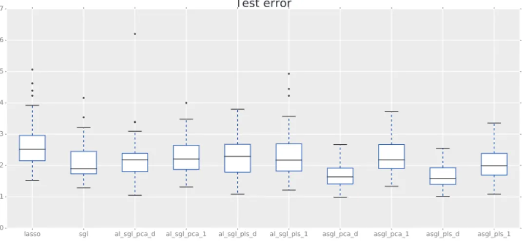
Figure 2: Simulation 1. Dataset with non-zero variables spread along many groups. 225 variables. Box-plots showing the test error of the different models.
Case 2: 625 variables
There are25groups of size25each, a total number of625variables. Among these groups, 7 groups with8 significant variables each are defined, a total number of56significant variables. Forl∈ {1. . . ,25}, coefficients inside each group are defined as,
⎧ ⎪ ⎪ ⎪ ⎨ ⎪ ⎪ ⎪ ⎩ βl = (1,2, . . . ,8,0, . . . ,0 17 ), l= 1, . . . ,7 βl = (0 , . . . ,0 25 ), l= 8, . . . ,25.
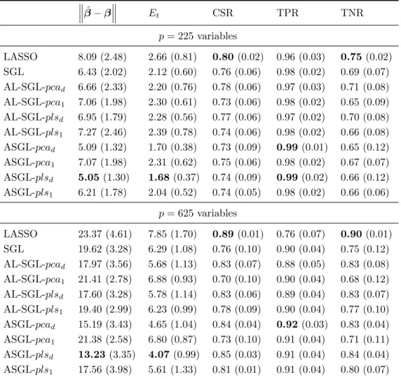
The results from this simulation scheme are displayed in Table 1. The best results are obtained by the ASGL model using plsd weights, closely followed bypcadweights. These models outperforms LASSO and SGL both in terms of the distance between predicted and trueβ, and in terms of the test error Et, improving prediction accuracy. Given that LASSO enhances individual sparsity, LASSO solutions are more sparse than the solutions ob-tained by the proposed models models, and this is shown in the TNR values. However, the proposed models produce a better selection of the truly signif-icant variables, fact that is displayed by the TPR values. If the number of
Table 1: Simulation 1. Dataset with non-zero variables spread along many groups, and 100/100/5000 train/validate/test observations. Experiments run 50 times and displayed as mean value, with standard deviations given in parenthesis ˆ β−β Et CSR TPR TNR p= 225variables LASSO 8.09 (2.48) 2.66 (0.81) 0.80(0.02) 0.96 (0.03) 0.75(0.02) SGL 6.43 (2.02) 2.12 (0.60) 0.76 (0.06) 0.98 (0.02) 0.69 (0.07) AL-SGL-pcad 6.66 (2.33) 2.20 (0.76) 0.78 (0.06) 0.97 (0.03) 0.71 (0.08) AL-SGL-pca1 7.06 (1.98) 2.30 (0.61) 0.73 (0.06) 0.98 (0.02) 0.65 (0.09) AL-SGL-plsd 6.95 (1.79) 2.28 (0.56) 0.77 (0.06) 0.97 (0.02) 0.70 (0.08) AL-SGL-pls1 7.27 (2.46) 2.39 (0.78) 0.74 (0.06) 0.98 (0.02) 0.66 (0.08) ASGL-pcad 5.09 (1.32) 1.70 (0.38) 0.73 (0.09) 0.99(0.01) 0.65 (0.12) ASGL-pca1 7.07 (1.98) 2.31 (0.62) 0.75 (0.06) 0.98 (0.02) 0.67 (0.07) ASGL-plsd 5.05(1.30) 1.68(0.37) 0.74 (0.09) 0.99(0.02) 0.66 (0.12) ASGL-pls1 6.21 (1.78) 2.04 (0.52) 0.74 (0.05) 0.98 (0.02) 0.66 (0.06) p= 625variables LASSO 23.37 (4.61) 7.85 (1.70) 0.89(0.01) 0.76 (0.07) 0.90(0.01) SGL 19.62 (3.28) 6.29 (1.08) 0.76 (0.10) 0.90 (0.04) 0.75 (0.12) AL-SGL-pcad 17.97 (3.56) 5.68 (1.13) 0.83 (0.07) 0.88 (0.05) 0.83 (0.08) AL-SGL-pca1 21.41 (2.78) 6.88 (0.93) 0.70 (0.10) 0.90 (0.04) 0.68 (0.12) AL-SGL-plsd 17.60 (3.28) 5.78 (1.14) 0.83 (0.06) 0.89 (0.04) 0.83 (0.07) AL-SGL-pls1 19.40 (2.99) 6.23 (0.99) 0.78 (0.09) 0.90 (0.04) 0.77 (0.10) ASGL-pcad 15.19 (3.43) 4.65 (1.04) 0.84 (0.04) 0.92(0.03) 0.83 (0.04) ASGL-pca1 21.38 (2.58) 6.80 (0.87) 0.73 (0.10) 0.91 (0.04) 0.71 (0.11) ASGL-plsd 13.23(3.35) 4.07(0.99) 0.85 (0.03) 0.91 (0.04) 0.84 (0.04) ASGL-pls1 17.56 (3.98) 5.61 (1.33) 0.81 (0.01) 0.91 (0.04) 0.80 (0.07)
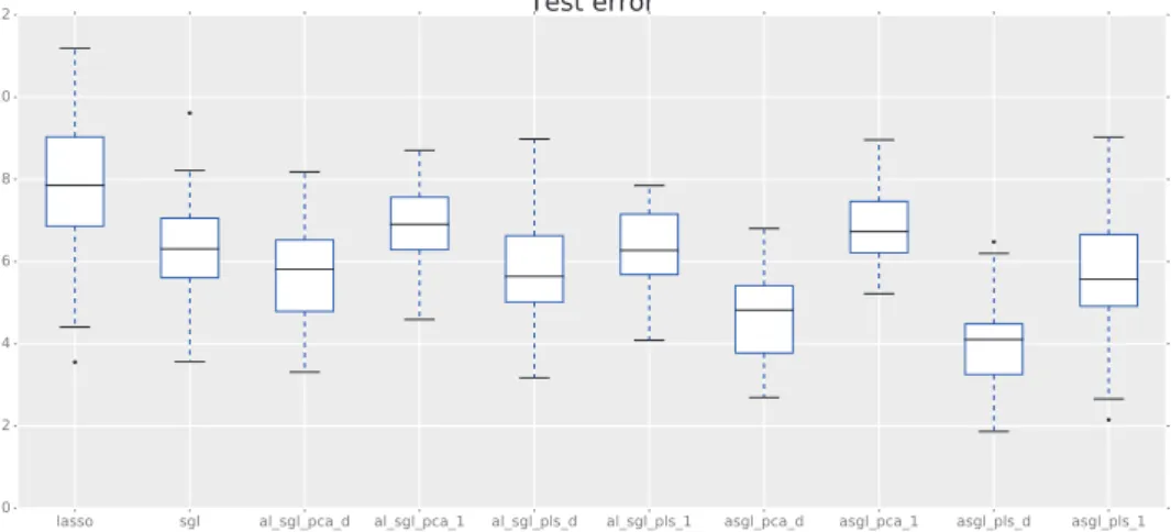
Figure 3: Simulation 1. Dataset with non-zero variables spread along many groups. 625 variables. Box-plots showing the test error of the different models.
variables is increased, the difference in performance between the proposed models, and LASSO and SGL gets larger, indicating that the performance of the proposed models is better than LASSO and SGL as the number of variables increase. Figures 2 and 3 display box-plots of the test error Et for the different models, showing that the spread of Et is much smaller in the ASGLplsdandpcadthan in the LASSO and SGL, indicating that these models provide more stable solutions in terms of prediction accuracy. A sec-ond simulation example in which there are a few groups that account for all the significant variables is shown.
5.2 Simulation 2: dense distribution of significant variables
Case 1: 225 variables
There are15groups of size15each, a total number of225variables. Among these groups, we define 3 groups with 15 significant variables each, a total number of45significant variables. Forl∈ {1. . . ,15}, coefficients inside each group are defined as,
⎧ ⎪ ⎨ ⎪ ⎩ βl = (1,2, . . . ,15), l= 1, . . . ,3 βl = (0, . . . ,0 15 ), l= 4, . . . ,15.
Figure 4: Simulation 2. Dataset with non-zero variables concentrated in a small number of fully significant groups. 225 variables. Box-plots showing the test error of the different models.
Case 2: 625 variables
There are25groups of size25each, a total number of625variables. Among these groups,3 groups with25 significant variables each are defined, a total number of75significant variables. Forl∈ {1. . . ,25}, coefficients inside each group are defined as,
⎧ ⎪ ⎨ ⎪ ⎩ βl = (1,2, . . . ,25), l= 1, . . . ,3 βl = (0 , . . . ,0 25 ), l= 4, . . . ,25.
The results from this simulation scheme are displayed in Table 2. Simi-larly to the situation displayed in Section 5.1, the ASGL model usingplsdor
pcadweights shows the best results in terms of the distance between predicted and trueβ, and the value ofEt. It is worth saying that under a more "com-pact" distribution of the significant variables in a small number of groups, the proposed methods show a great improvement in terms of prediction ac-curacy compared to LASSO and SGL. Figures 4 and 5 display box-plots of test error valueEtshowing, as in the previous simulation scheme, that ASGL models with plsd or pcad weights also provide more stable results in terms of spread.
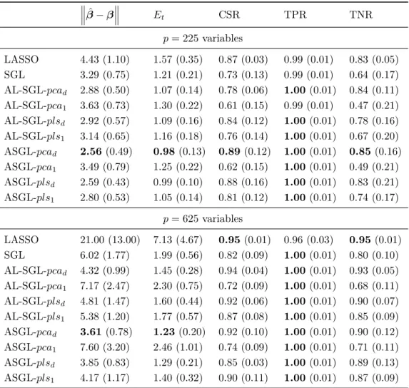
Table 2: Simulation 2. Dataset with non-zero variables concen-trated in a small number of fully significant groups, and 100/100/5000
train/validate/test observations. Experiments run 50 times and displayed as mean value, with standard deviations given in parenthesis
ˆ β−β Et CSR TPR TNR p= 225 variables LASSO 4.43 (1.10) 1.57 (0.35) 0.87 (0.03) 0.99 (0.01) 0.83 (0.05) SGL 3.29 (0.75) 1.21 (0.21) 0.73 (0.13) 0.99 (0.01) 0.64 (0.17) AL-SGL-pcad 2.88 (0.50) 1.07 (0.14) 0.78 (0.06) 1.00(0.01) 0.84 (0.11) AL-SGL-pca1 3.63 (0.73) 1.30 (0.22) 0.61 (0.15) 0.99 (0.01) 0.47 (0.21) AL-SGL-plsd 2.92 (0.57) 1.09 (0.16) 0.84 (0.12) 1.00(0.01) 0.78 (0.16) AL-SGL-pls1 3.14 (0.65) 1.16 (0.18) 0.76 (0.14) 1.00(0.01) 0.67 (0.20) ASGL-pcad 2.56(0.49) 0.98 (0.13) 0.89(0.12) 1.00(0.01) 0.85(0.16) ASGL-pca1 3.49 (0.79) 1.25 (0.22) 0.62 (0.15) 1.00(0.01) 0.49 (0.21) ASGL-plsd 2.59 (0.43) 0.99 (0.10) 0.88 (0.16) 1.00(0.01) 0.83 (0.21) ASGL-pls1 2.80 (0.53) 1.05 (0.14) 0.81 (0.12) 1.00(0.01) 0.74 (0.17) p= 625 variables LASSO 21.00 (13.00) 7.13 (4.67) 0.95(0.01) 0.96 (0.03) 0.95(0.01) SGL 6.02 (1.77) 1.99 (0.56) 0.82 (0.09) 1.00(0.01) 0.80 (0.10) AL-SGL-pcad 4.32 (0.99) 1.45 (0.28) 0.94 (0.04) 1.00(0.01) 0.93 (0.05) AL-SGL-pca1 7.17 (2.47) 2.30 (0.75) 0.72 (0.09) 1.00(0.01) 0.68 (0.11) AL-SGL-plsd 4.81 (1.47) 1.60 (0.44) 0.92 (0.06) 1.00(0.01) 0.90 (0.07) AL-SGL-pls1 5.38 (1.20) 1.77 (0.57) 0.87 (0.08) 1.00(0.01) 0.85 (0.09) ASGL-pcad 3.61(0.78) 1.23 (0.20) 0.92 (0.10) 1.00(0.01) 0.90 (0.12) ASGL-pca1 7.60 (3.20) 2.46 (1.01) 0.74 (0.09) 1.00(0.01) 0.71 (0.11) ASGL-plsd 3.85 (0.83) 1.29 (0.21) 0.85 (0.03) 1.00(0.01) 0.89 (0.13) ASGL-pls1 4.17 (1.17) 1.40 (0.32) 0.90 (0.11) 1.00(0.01) 0.87 (0.09)
Figure 5: Simulation 2. Dataset with non-zero variables concentrated in a small number of fully significant groups. 625 variables. Box-plots showing the test error of the different models.
Based on the simulations described in Sections 5.1 and 5.2, we conclude that the best performance is achieved by ASGL models with plsd or pcad weights.
5.3 Simulation 3: n > p
This simulation defines a low-dimensional scenario that studies the perfor-mance of the ASGL model withplsdandpcadweights compared to an ASGL model with weights from an unpenalized model. The simulation scheme con-siders200/200/5000observations in the train / validate / test samples, and 100 variables divided into 10 groups of size 10 each. Two different cases depending on the distribution of the significant variables are considered:
Case 1: Sparse distribution of variables
Here,5 groups with 6 significant variables each are defined, a total number of 30 significant variables. Forl∈ {1. . . ,10}, coefficients inside each group are defined as,
⎧ ⎪ ⎪ ⎪ ⎨ ⎪ ⎪ ⎪ ⎩ βl = (1,2, . . . ,6,0 , . . . ,0 4 ), l= 1, . . . ,5 βl = (0 , . . . ,0 10 ), l= 6, . . . ,10.
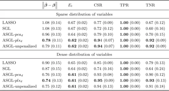
Table 3: Simulation 3. Dataset with 200/200/5000 train/validate/test ob-servations. Experiments run 50 times and displayed as mean value, with standard deviations given in parenthesis
ˆ β−β Et CSR TPR TNR
Sparse distribution of variables
LASSO 1.08 (0.14) 0.67 (0.02) 0.77 (0.09) 1.00(0.00) 0.67 (0.12) SGL 1.08 (0.13) 0.67 (0.02) 0.72 (0.12) 1.00(0.00) 0.60 (0.16) ASGL-pcad 0.96 (0.13) 0.64 (0.02) 0.79 (0.10) 1.00(0.00) 0.70 (0.15) ASGL-plsd 0.78(0.11) 0.62(0.02) 0.94 (0.07) 1.00(0.00) 0.92(0.09) ASGL-unpenalized 0.79 (0.11) 0.62(0.02) 0.94(0.07) 1.00(0.00) 0.92(0.09)
Dense distribution of variables
LASSO 0.90 (0.15) 0.65 (0.02) 0.85 (0.09) 1.00(0.00) 0.79 (0.13) SGL 0.87 (0.15) 0.64 (0.02) 0.74 (0.16) 1.00(0.00) 0.64 (0.24) ASGL-pcad 0.76 (0.13) 0.61(0.02) 0.93 (0.08) 1.00(0.00) 0.90 (0.12) ASGL-plsd 0.74(0.13) 0.61(0.02) 0.95(0.09) 1.00(0.00) 0.93(0.13) ASGL-unpenalized 0.75 (0.12) 0.61(0.02) 0.94 (0.13) 1.00(0.00) 0.91 (0.18)
Case 2: Dense distribution of variables
Here,3groups with10significant variables each are defined, a total number of 30 significant variables. Forl∈ {1. . . ,10}, coefficients inside each group are defined as,
βl = (1,2, . . . ,10), l= 1, . . . ,3 βl = (0, . . . ,0 | {z } 10 ), l= 4, . . . ,10.
Table 3 shows the results from this simulation. In both cases, the sparse and the dense distribution of variables, the best results in terms of the dis-tance between predicted and true β, and in terms of the test error Et are
obtained by the ASGL model usingplsd, closely followed by the ASGL model
with unpenalized model weights and by ASGL with pcad weights. All the
models achieve a TPR of 1.00, indicating that all the models selected cor-rectly all the significant variables. However, the largest TNR is achieved by ASGL with plsd or unpenalized weights, indicating that these models tend
to select less non-important variables than the other models. This simula-tion example shows that even though the proposals made in Secsimula-tion 4 are
specially suited for high-dimensional scenarios, the performance achieved in low-dimensional scenarios is very good, and is at least as good as the per-formance of the models with unpenalized weights.
6
Real application
The performance of the ASGL estimator is shown here using a genomic dataset first reported in [Scheetz et al., 2006]. The dataset consists of 120
twelve-week-old male offspring animals chosen for tissue harvesting from the eyes and for micro-array analysis. The dataset contains expression values from31042 different probe-sets (Affymetric GeneChip Rat Genome 230 2.0
Array) on a logarithmic scale. As described in [Huang et al., 2008] and [Wang et al., 2012], a two-steps preprocessing is performed, selecting, among the
31042 probe-sets, the ones that are sufficiently expressed, and sufficiently variable. A probe is considered to be sufficiently expressed if the maximum expression value observed for that probe among the 120animals is greater than the25-thpercentile of the entire set of RMA expression values. A probe is considered to be sufficiently variable if it shows at least2-fold variation in the expression value among the120rats. There are18986probes that meet these criteria.
We study how expression level of gene TRIM32, corresponding to probe
1389163_at, is related to expression levels at other probes. [Chiang et al., 2006] pointed out that gene TRIM32 was found to cause Bardet-Biedl syn-drome, a disease of multiple organ systems including the retina. [Scheetz et al., 2006] said: “Any genetic element that can be shown to alter the ex-pression of a specific gene or gene family known to be involved in a specific disease is itself an excellent candidate for involvement in the disease, either primarily or as a genetic modifier.” Here the sample size is120(the number of animals selected for micro-array analysis), and the number of covariates (probes that pass the preprocessing steps) is18985. The correlation coeffi-cients of the 18985 probes and the probe corresponding to gene TRIM32 is calculated, and the genes in which the absolute value of the correlation ex-ceeds0.5 are selected. There are 3734probes meeting this criteria. Finally, this dataset is standardized. Only a few genes are expected to be related to gene TRIM32, making this a high-dimensional sparse problem.
individu-ally. The problem of grouping genes based on a medical criteria is nowadays under intense study, and it is possible to find some group structures for hu-man genetic information based, for example, in cytogenetic positions [Sub-ramanian et al., 2005]. It is interesting to remark that groups built based on biological criteria are usually formed just by a few dozens of genes. For example, in the case of groups based on cytogenetic positions, groups av-eraged 30 genes, as stated in [Simon et al., 2013]. However, these group structures are not available for all the genetic information, and to the best of our knowledge there is no genetic grouping alternative for the dataset under study here.
We address the grouping problem from an statistical perspective, using principal components analysis to create groups of genes that are similar. It is worth to remark that in Section 4.1 PCA was used for estimating the ASGL weights, while here it will be used for variable clustering.
Variable clustering using PCA
1. Given a matrix of covariates X ∈ Rn×p as in Section 4.1, obtain the
matrix of principal componentsQ∈Rp×rX ∈
Rn×pdefined in Section
4.1.
2. Consider r possible groups, as many as principal components.
3. Each principal componentqi∈Q,i∈1, . . . , r, is a linear combination
of the original variables fromX. Assign each original variable to the group associated to the principal component in which that variable had its maximum weight (in absolute value).
The intuition behind this process is that variables with a large weight in the same principal component are likely to be related and should be included in the same group.
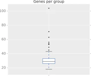
In the case of the dataset used in this section, there are120observations from 3734 different genes. The maximum rank of X here is 120, for this reason120possible groups are initially considered. Each gene is assigned to the group associated to the principal component in which that gene had its maximum weight. No gene was assigned to one of the groups, and therefore
119 groups averaging 32 genes per group are created this way. It is worth remarking that the average group size obtained based on this proposal is
Figure 6: Gene expression data of rat eye disease. Box-plot showing the sizes of the groups built using PCA.
Table 4: Gene expression data of rat eye disease. 20random dataset divisions were considered. Results displayed as mean value, with standard errors in parenthesis. Et # Variables selected LASSO 0.34 (0.08) 18.9 (15.4) SGL 0.31 (0.07) 189.5 (156.6) ASGL-pcad 0.28 (0.06) 56.35 (70.86) ASGL-plsd 0.29 (0.06) 101.7 (85.56)
close to the expected group size in terms of the cytogenetic position. Figure 6 shows a box-plot of the group sizes.
The dataset is randomly divided into80/20/20train / validate / test ob-servations and LASSO, SGL, ASGLplsdand ASGL pcadmodels are solved. For each model, the test error Et and the significant variables selected are obtained. This process is repeated 20times as a way to gain stability.
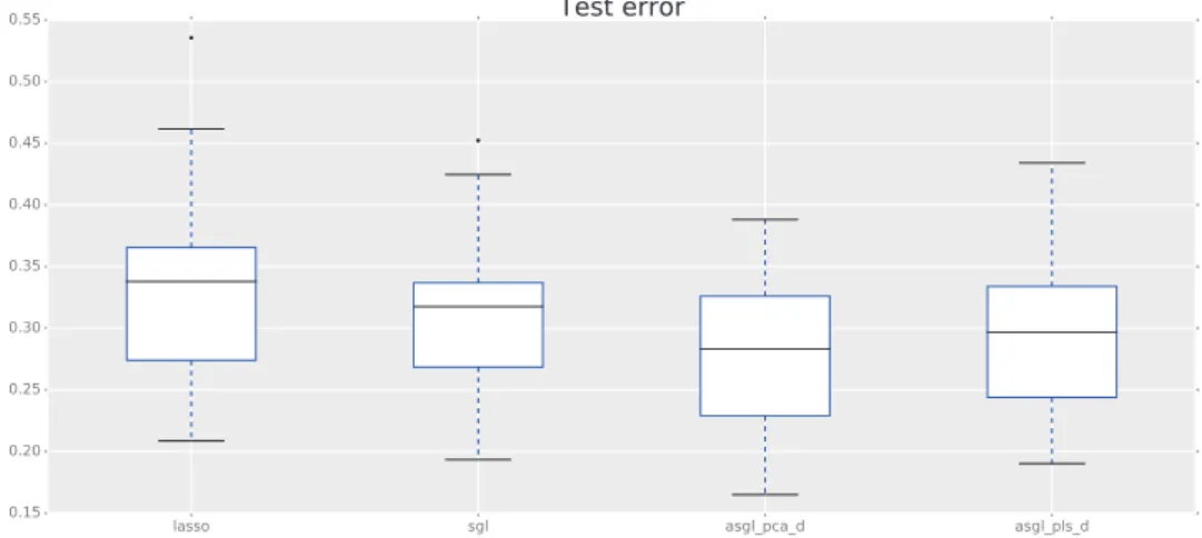
The results obtained are shown in Table 4. The best results in terms of the test error are obtained by the proposed ASGL models. LASSO offers a test error approximately 20% greater while SGL test error is 11% greater. Figure 7 displays box-plots of the test errorEt, showing that the spread ofEt is also smaller in the proposed ASGL models providing more stable results. Figure 8 displays box-plots of the number of genes each model selected as
Figure 7: Gene expression data of rat eye disease. 20 random dataset divi-sions were considered. Box-plot showing the test error.
Figure 8: Gene expression data of rat eye disease. 20 random dataset divi-sions were considered. Box-plot showing the number of significant genes.
Figure 9: Gene expression data of rat eye disease. 20 random dataset divi-sions were considered. Heatmap showing the probability of being a significant gene. Each row represents a model and each column represents a gene.
significant. The LASSO is the one offering more sparse solutions, using only
19 variables (in mean) per model. SGL is the one using the largest number of variables, approximately190, and also the one with the largest variability in this metric. Both ASGL pcad and ASGL plsd selected a smaller number
of variables than SGL but still larger than LASSO, and they achieve the best prediction results of the four models.
Given that we have the results obtained from20repetitions, it is possible to count the number of times each gene has been selected as significant by one of the models in any of the repetitions. Dividing this number by the total number of repetitions, a sort of "probability of being a significant gene" associated to each gene for each model considered is obtained. Out of the
3734 genes in the dataset, 1612 genes were selected at least one time by any of the models in any of the repetitions (the majority being selected by SGL models). Figure 9 shows the probability of being a significant gene for these1612variables and for each model. Rows represent the different models considered and columns represent each gene. Genes are sorted based on the probabilities obtained in the ASGL model withpcad weights.
Table 5: Gene expression data of rat eye disease. 20 random dataset divi-sions were considered. Number of genes above the probability threshold for different quantile levels.
Number of genes above the probability threshold τ= 0.3 τ = 0.5 τ = 0.7 Three quantiles
LASSO 0 1 1 0
SGL 19 35 17 0
ASGL-pcad 23 9 17 7
ASGL-plsd 41 17 37 9
models reach a probability of significance above the threshold, showing no stability on the gene selection along the20repetitions, and anticipating prob-lems with possible further biological interpretation of the statistical results. In the case of the SGL model, 35 genes are above the probability thresh-old, being 0.6 the maximum probability achieved. On the other hand, the ASGL model with plsd weights includes 17 genes with probabilities above
the threshold with a maximum probability value of 0.75, and the ASGL model withpcadweights has 9genes above the probability threshold with a
maximum probability value of 0.9, showing more stability on the selection along the 20 repetitions and possibly better biological interpretation of the results than the other models.
Results displayed in Table 4 and Figure 9 have been obtained using esti-mators of the median of the response variable, however, it can be interesting to compare the genes selected at different quantiles. For this reason, the pro-cess described above is repeated and LASSO, SGL, ASGL plsd and ASGL
pcad models are solved for quantile levels τ = 0.3 and τ = 0.7,
obtain-ing probabilities of beobtain-ing a significant gene for each quantile level and each model. Considering a probability threshold of0.5, Table 5 show the number of genes above the probability threshold for each quantile, and also the num-ber of genes in the same model that have been selected along the different quantile levels.
The LASSO model shows no stability on the variable selection, having only one gene above the threshold forτ = 0.5andτ = 0.7, and no gene with probability of being significant above 0.5 on the three quantiles simultane-ously. The SGL show some stability across the 20 repetitions considering
each quantile independently, but when considering all the quantiles simulta-neously it has no gene above the probability threshold. On the other hand, in the case of the ASGLplsdmodel,9genes had a probability of being
signif-icant greater than 0.5in the 3 quantiles, and in the case of the ASGLpcad
models, 7 genes fulfilled this, showing more robust results than the other estimators.
We conclude that the best results in this real dataset study are provided by the ASGL model with pcad weights, given that this model is the one
with the smallest prediction error and showing great stability on the gene selection.
7
Computational aspects
All the simulations and data analysis commented in Sections 5 and 6 were run in a cluster node with two Intel (R) Xeon(R) CPU E5-2630 v3 (2.4GHz, 20MB Smart Cache) processors, with 32Gb of RAM memory running Cen-tOS 6.5 Final (Rocks 6.1.1 Sand Boa). The computation itself has been developed in Python 2.7.15 (Anaconda Inc.) All the optimization problems have been solved using the CVXPY optimization framework for Python [Di-amond and Boyd, 2016] and the open source solver ECOS [Domahidi et al., 2013].
8
Conclusion
In this paper the definition of the SGL estimator has been extended to the QR framework. A new estimator for quantile regression based on the usage of adaptive weights, the adaptive sparse group LASSO in quantile regres-sion has also been proposed. Typically in the literature the weights of the adaptive estimators are defined based on non-penalized models, however, this definition limits the usage of the adaptive estimators to low-dimensional scenarios. As a solution to this problem, four weight calculation alternatives that can be used in high-dimensional scenarios when working with adaptive estimators are proposed. We test the performance of the proposed alter-natives in a set of synthetic data scenarios that includes high-dimensional and low-dimensional examples, showing that it is a competitive option in both situations. The performance of the proposed work is also studied in
a real dataset including gene expression values of rat eye disease. We com-pare the results of the proposed work with LASSO, SGL and ASGL with weights from unpenalized models (the last one only in the low-dimensional examples). Based on the synthetic datasets both ASGLplsdand ASGLpcad
achieve very good results, as described in Section 5, however, when dealing with the real dataset, the ASGL pcad estimator achieved better results in
terms of prediction error and stability of the variables selected. For this reason we conclude that the ASGLpcadprovides the best results among the
options proposed in this work.
This work has risen some questions that will require further investigation. One interesting problem is this of the optimization of the hyper-parameters. In this work we make use of grid-search, but it is worth commenting that new hyper-parameter tuning alternatives have appeared in recent years [Laria et al., 2019], and it can be interesting to investigate the usage of this or other options in the optimization of the parameters of the proposed models here.
As commented in Section 3, the general tendency found in the literature when working with adaptive estimators is to work in order to demonstrate that the estimator fulfills the so-called oracle properties. This demonstration is usually based on the usage of the un-penalized model estimator, step that can only be achieved in low-dimensional scenarios. Actually, this requirement can be reformulated, changing the usage of the un-penalized estimator by any other root-n consistent estimator We thus conjecture that the ASGL plsd and ASGL pcad estimators, as they are used in this work, may be
root-n consistent, fulfilling this way the oracle properties. This conjecture however will require further research.
9
Acknowledgments
In this research we have made use of Uranus, a supercomputer cluster located at University Carlos III of Madrid and funded jointly by EU-FEDER funds and by the Spanish Government via the National Projects No. UNC313-4E-2361, No. ENE2009-12213- C03-03, No. ENE2012-33219 and No. ENE2015-68265-P. This research was partially supported by research grants and Project ECO2015-66593-P from Ministerio de Economía, Industria y Competitivi-dad, Project MTM2017-88708-P from Ministerio de Economía y
Competi-tividad, FEDER funds and Project IJCI-2017-34038 from Agencia Estatal de Investigación, Ministerio de Ciencia, Innovación y Universidades.
References
[Chatterjee et al., 2011] Chatterjee, S., Banerjee, A., Chatterjee, S., and Ganguly, A. R. (2011). Sparse Group Lasso for Regression on Land Cli-mate Variables. In 2011 IEEE 11th International Conference on Data Mining Workshops, pages 1–8. IEEE.
[Chiang et al., 2006] Chiang, A. P., Beck, J. S., Yen, H.-J., Tayeh, M. K., Scheetz, T. E., Swiderski, R. E., Nishimura, D. Y., Braun, T. A., Kim, K.-Y. A., Huang, J., Elbedour, K., Carmi, R., Slusarski, D. C., Casavant, T. L., Stone, E. M., and Sheffield, V. C. (2006). Homozygosity mapping with SNP arrays identifies TRIM32, an E3 ubiquitin ligase, as a Bardet-Biedl syndrome gene (BBS11). Proceedings of the National Academy of Sciences, 103(16):6287–6292.
[Ciuperca, 2017] Ciuperca, G. (2017). Adaptive fused LASSO in grouped quantile regression. Journal of Statistical Theory and Practice, 11(1):107– 125.
[Ciuperca, 2019] Ciuperca, G. (2019). Adaptive group LASSO selection in quantile models. Statistical Papers, 60(1):173–197.
[Diamond and Boyd, 2016] Diamond, S. and Boyd, S. (2016). CVXPY: A Python-Embedded Modeling Language for Convex Optimization.
arXiv:1603.00943.
[Domahidi et al., 2013] Domahidi, A., Chu, E., and Boyd, S. (2013). ECOS: An SOCP Solver for Embedded Systems. InEuropean Control Conference (ECC).
[Fan and Li, 2001] Fan, J. and Li, R. (2001). Variable Selection via Non-concave Penalized Likelihood and Its Oracle Properties. Journal of the American Statistical Association, 96(456):1348–1360.
[Friedman et al., 2010] Friedman, J., Hastie, T., and Tibshirani, R. (2010). A note on the group lasso and a sparse group lasso. arXiv:1001.0736v1.
[Huang et al., 2008] Huang, J., Ma, S., and Zhang, C.-H. (2008). Adaptive Lasso for Sparse High-dimensional Regression. Statistica Sinica, 1(374):1– 28.
[Koenker, 2005] Koenker, R. (2005). Quantile Regression. Cambridge uni-versity Press.
[Koenker and Bassett, 1978] Koenker, R. and Bassett, G. (1978). Regression Quantiles. Econometrica, 46(1):33–50.
[Laria et al., 2019] Laria, J. C., Aguilera-Morillo, M. C., and Lillo, R. E. (2019). An iterative sparse-group lasso. Journal of Computational and Graphical Statistics, :1–21. doi:10.1080/10618600.2019.1573687
[Li and Zhu, 2008] Li, Y. and Zhu, J. (2008). L1- -Norm Quantile Regres-sion. Journal of Computational and Graphical Statistics, 17(1):1–23. [Nardi and Rinaldo, 2008] Nardi, Y. and Rinaldo, A. (2008). On the
asymp-totic properties of the group lasso estimator for linear models. Electronic Journal of Statistics, 2(0):605–633.
[Poignard, 2018] Poignard, B. (2018). Asymptotic theory of the adaptive Sparse Group Lasso. Annals of the Institute of Statistical Mathematics. [Scheetz et al., 2006] Scheetz, T. E., Kim, K.-Y. A., Swiderski, R. E., Philp,
A. R., Braun, T. A., Knudtson, K. L., Dorrance, A. M., DiBona, G. F., Huang, J., Casavant, T. L., Sheffield, V. C., and Stone, E. M. (2006). Reg-ulation of gene expression in the mammalian eye and its relevance to eye disease. Proceedings of the National Academy of Sciences, 103(39):14429– 14434.
[Simon et al., 2013] Simon, N., Friedman, J., Hastie, T., and Tibshirani, R. (2013). A sparse-group lasso. Journal of Computational and Graphical Statistics, 22(2):231–245.
[Subramanian et al., 2005] Subramanian, A., Tamayo, P., Mootha, V. K., Mukherjee, S., Ebert, B. L., Gillette, M. A., Paulovich, A., Pomeroy, S. L., Golub, T. R., Lander, E. S., and Mesirov, J. P. (2005). Gene set en-richment analysis: A knowledge-based approach for interpreting genome-wide expression profiles.Proceedings of the National Academy of Sciences, 102(43):15545–15550.
[Tibshirani, 1996] Tibshirani, R. (1996). Regression Shrinkage and Selection via the Lasso. Journal of the Royal Statistical Society. Series B (Method-ological), 58(1):267–288.
[Wang et al., 2012] Wang, L., Wu, Y., and Li, R. (2012). Quantile regres-sion for analyzing heterogeneity in ultra-high dimenregres-sion. Journal of the American Statistical Association, 107(497):214–222.
[Wright et al., 2010] Wright, J., Ma, Y., Mairal, J., Sapiro, G., Huang, T. S., and Yan, S. (2010). Sparse Representation for Computer Vision and Pat-tern Recognition. Proceedings of the IEEE, 98(6):1031–1044.
[Wu and Liu, 2009] Wu, Y. and Liu, Y. (2009). Variable selection in quantile regression. Statistica Sinica, 19(2):801–817.
[Yuan and Lin, 2006] Yuan, M. and Lin, Y. (2006). Model selection and estimation in regression with grouped variables. Journal of the Royal Statistical Society. Series B (Methodological), 68(1):49–67.
[Zhao et al., 2014] Zhao, W., Zhang, R., and Liu, J. (2014). Sparse group variable selection based on quantile hierarchical Lasso. Journal of Applied Statistics, 41(8):1658–1677.
[Zhou and Zhu, 2010] Zhou, N. and Zhu, J. (2010). Group variable selection via a hierarchical lasso and its oracle property.Statistics and Its Interface, 3:557–574.
[Zou, 2006] Zou, H. (2006). The Adaptive Lasso and Its Oracle Properties.