End-to-End Neural Speech Translation

(1)

End-to-End Neural Speech

Translation

zur Erlangung des akademischen Grades eines

Doktors der Ingenieurwissenschaften von der KIT-Fakultät für Informatik des Karlsruher Instituts für Technologie (KIT)

genehmigte

Dissertation

von

Matthias Sperber

aus Karlsruhe

Tag der m¨undlichen Pr¨ufung: 9.1.2019

Erster Gutachter: Prof. Dr. Alexander Waibel

(2)

(3)

Ich erkläre hiermit, dass ich die vorliegende Arbeit selbständig verfasst und keine anderen als die angegebenen Quellen und Hilfsmittel verwendet habe, sowie dass ich die wörtlich oder inhaltlich übernommenen Stellen als solche kenntlich gemacht habe und die Satzung des KIT, ehem. Universität Karlsruhe (TH), zur Sicherung guter wissenschaftlicher Praxis in der jeweils gültigen Fassung beachtet habe.

Karlsruhe, den 14.11.2018

(4)

(5)

Abstract

The goal of this thesis is to develop improved methods for the task of speech translation. Speech translation takes audio signals of speech as input and produces text translations as output, with diverse applications that reach from dialog-based translation in limited domains to automatic translation of academic lectures. A main challenge and reason why current speech translation systems often produce unsatisfactory results is the division of the task into independent recognition and translation steps, leading to the well-known error propagation problem. In this thesis, we use recent neural modeling techniques to tighten the speech translation pipeline and, in the extreme, replace the cascade by models that directly generate translations from speech without an intermediate step. The overarching goal of all proposed approaches is the reduction or prevention of the error propagation problem.

As a starting point, we analyze the state-of-the-art for attentional speech recognition models, and develop a new model with a self-attentional acoustic model component. We show that this reduces training time significantly and enables inspection and linguistic interpretation of models that have previously often been described as black box approaches. Equipped with such a model, we then turn to the problem of speech translation, first from the viewpoint of a cascade, where we wish to translate the output of a speech recognizer as accurately as possible. This requires dealing with errors from the speech recognizer, which we achieve by noising the training data, leading to improved robustness of the translation component. A second approach is to explicitly handle competing recognition hypotheses during translation, which we accomplish through a novel lattice-to-sequence model, achieving substantial improvements in translation accuracy.

Direct models for speech translation are a promising new approach that does not divide the process into two independent steps. This requires direct data in which spoken utterances are paired with a textual translation, which is different from cascaded models in which both model components are trained on independent speech recognition and

(6)

machine translation corpora. Sequence-to-sequence models can now be trained on such direct data, and have in fact been used along these lines by some research groups, although with only inconsistent reported improvements. In this thesis, we show that whether such models outperform traditional models critically depends on the amount of available direct data, an observation that can be explained by the more complex direct mapping between source speech inputs and target text outputs. This puts direct models at a disadvantage in practice, because we usually possess only limited amounts of direct speech translation data, but have access to much more abundant data for cascaded training. A straight-forward potential solution for incorporating all available data is multi-task training, but we show that this is ineffective and not able to overcome the data disadvantage of the direct model. As a remedy, we develop a new two-stage model that naturally decomposes into two modeling steps akin to the cascade, but is end-to-end trainable and reduces the error propagation problem. We show that this model outperforms all other approaches under ideal data conditions, and is also much more effective at exploiting auxiliary data, closing the gap to the cascaded model in realistic situations. This shows for the first time that end-to-end trainable speech translation models are a practically relevant solution to speech translation, and are able to compete with or outperform traditional approaches.

(7)

Zusammenfassung

Diese Arbeit besch¨aftigt sich mit Methoden zur Verbesserung der automatischen ¨

Ubersetzung gesprochener Sprache (kurz: Speech Translation). Die Eingabe ist hierbei ein akustisches Signal, die Ausgabe ist der zugeh¨orige Text in einer anderen Sprache. Die Anwendungen sind vielf¨altig und reichen u.a. von dialogbasierten

¨

Ubersetzungssystemen in begrenzten Dom¨anen bis hin zu vollautomatischen Vorlesungs¨ubersetzungssystemen.

Speech Translation ist ein komplexer Vorgang der in der Praxis noch viele Fehler produziert. Ein Grund hierfür ist die Zweiteilung in Spracherkennungskomponente und Übersetzungskomponente: beide Komponenten produzieren für sich genommen eine gewisse Menge an Fehlern, zusätzlich werden die Fehler der ersten Komponente an die zweite Komponente weitergereicht (sog. Error Propagation) was zusätzliche Fehler in der Ausgabe verursacht. Die Vermeidung des Error Propagation Problems ist daher grundlegender Forschungsgegenstand im Speech Translation Bereich.

In der Vergangenheit wurden bereits Methoden entwickelt, welche die Schnittstelle zwischen Spracherkenner und ¨Ubersetzer verbessern sollen, etwa durch Weiterreichen mehrerer Erkennungshypothesen oder durch Kombination beider Modelle mittels Finite State Transducers. Diese basieren jedoch weitgehend auf veralteten, statistischen

¨

Ubersetzungsverfahren, die mittlerweile fast vollst¨andig durch komplett neuronale Sequence-to-Sequence Modelle ersetzt wurden.

Die vorliegende Dissertation betrachtet mehrere Ansätze zur Verbesserung von Speech Translation, alle motiviert durch das Ziel, Error Propagation zu vermeiden, sowie durch die Herausforderungen und Möglichkeiten der neuen komplett neuronalen Modelle zur Spracherkennung und Übersetzung. Hierbei werden wir zum Teil völlig neuartige Modelle entwickeln und zum Teil Strategien entwickeln um erfolgreiche klassische Ideen auf neuronale Modelle zu übertragen.

Wir betrachten zun¨achst eine einfachere Variante unseres Problems, die Spracherkennung. Um Speech Translation Modelle zu entwickeln die komplett

(8)

auf neuronalen Sequence-to-Sequence Modellen basieren, müssen wir zunächst sicherstellen dass wir dieses einfachere Problem zufriedenstellend mit ähnlichen Modellen lösen können. Dazu entwickeln wir zunächst ein komplett neuronales Baseline Spracherkennungs-System auf Grundlage von Ergebnissen aus der Literatur, welches wir anschließend durch eine neuartige Self-Attentional Architektur erweitern. Wir zeigen dass wir hiermit sowohl die Trainingszeit verkürzen können, als auch bessere Einblicke in die oft als Blackbox beschriebenen Netze gewinnen und diese aus linguistischer Sicht interpretieren können.

Als nächstes widmen wir uns dem kaskadierten Ansatz zur Speech Translation. Hier nehmen wir an, dass eine Ausgabe eines Spracherkenners gegeben ist, und wir diese so akkurat wie möglich ubersetzen¨ wollen. Dazu ist es nötig, mit den Fehlern des Spracherkenners umzugehen, was wir erstens durch verbesserte Robustheit des Ubersetzers und zweitens durch Betrachten¨ alternativer Erkennungshypothesen erreichen. Die Verbesserung der Robustheit der

¨

Ubersetzungskomponente, unser erster Beitrag, erreichen wir durch das Verrauschen der Trainings-Eingaben, wodurch das Modell lernt, mit fehlerhaften Eingaben und insbesondere Spracherkennungsfehlern besser umzugehen. Zweitens entwickeln wir ein Lattice-to-Sequence Übersetzungsmodell, also ein Modell welches Wortgraphen als Eingaben erwartet und diese in eine übersetzte Wortsequenz überführt. Dies ermöglicht uns, einen Teil des Hypothesenraums des Spracherkenners, in Form eines eben solchen Wortgraphen, an den Spracherkenner weiterzureichen. Hierdurch hat die Übersetzungskomponente Zugriff auf verschiedene alternative Ausgaben des Spracherkenners und kann im Training lernen, daraus selbständig die zum Übersetzen optimale und weniger fehlerbehaftete Eingabe zu extrahieren.

Schließlich kommen wir zum finalen und wichtigsten Beitrag dieser Dissertation. Ein vielversprechender neuer Speech Translation Ansatz ist die direkte Modellierung, d.h. ohne explizite Erzeugung eines Transkripts in der Quellsprache als Zwischenschritt. Hierzu sind direkte Daten, d.h. Tonaufnahmen mit zugehörigen textuellen Übersetzungen nötig, im Unterschied zu kaskadierten Modellen, welche auf transkribierte Tonaufnahmen sowie davon unabhängigen parallelen übersetzten Texten trainiert werden. Erstmals bieten die neuen end-to-end trainierbaren Sequence-to-Sequence Modelle grundsätzlich die Möglichkeit dieses direkten Weges und wurden auch bereits von einigen Forschungsgruppen entsprechend getestet, jedoch sind die Ergebnisse teils widersprüchlich und es bleibt bisher unklar, ob man Verbesserungen gegenüber kaskadierten Systemen erwarten kann. Wir zeigen hier dass dies entscheidend von der Menge der verfügbaren Daten abhängt, was sich leicht dadurch erklären lässt

(9)

dass direkte Modellierung ein deutlich komplexeres Problem darstellt als der Weg ¨

uber zwei Schritte. Solche Situationen bedeuten im Maschinellen Lernen oftmals dass mehr Daten benötigt werden. Dies führt uns zu einem fundamentalen Problem dieses ansonsten sehr vielversprechenden Ansatzes, nämlich dass mehr direkte Trainingsdaten benötigt werden, obwohl diese in der Praxis sehr viel schwieriger zu sammeln sind als Trainingsdaten für traditionelle Systeme. Als Ausweg testen wir zunächst eine naheliegende Strategie, weitere traditionelle Daten ins direkte Modell-Training zu integrieren: Multi-Task Training. Dies stellt sich in unseren Experimenten allerdings als unzureichend heraus. Wir entwickeln daher ein neues Modell, das ähnlich einer Kaskade auf zwei Modellierungsschritten basiert, jedoch komplett durch Backpropagation trainiert wird und dabei bei der Übersetzung nur auf Audio-Kontextvektoren zurückgreift und damit nicht durch Erkennungsfehler beeinträchtigt wird. Wir zeigen dass dieses Modell erstens unter idealen Datenkonditionen bessere Ergebnisse gegenüber vergleichbaren direkten und kaskadierten Modellen erzielt, und zweitens deutlich mehr von zusätzlichen traditionellen Daten profitiert als die einfacheren direkten Modelle. Wir zeigen damit erstmals, dass end-to-end trainierbare Speech Translation Modelle eine ernst zu nehmende und praktisch relevante Alternative für traditionelle Ansätze sind.

(10)

(11)

Acknowledgements

First and foremost I would like to thank Prof. Alex Waibel for his guidance throughout my years as a PhD student, and for his research vision and ideas that made this thesis possible. I am also grateful for being given the opportunity to spend my early PhD years at NAIST in Japan. I am indebted to my co-advisor Prof. Satoshi Nakamura for much support and valuable advice, both during my stays at NAIST and afterwards. I would also like to express gratitude for countless discussions and practical help to Jan Niehues and Sebastian Stüker at KIT, and for all the support from Graham Neubig and Sakriani Sakti at both NAIST and CMU. Special thanks go to my colleagues from Karlsruhe: Eunah Cho, Stefan Constantin, Christian Fügen, Thanh-Le Ha, Michael Heck, Teresa Herrmann, Thilo Köhler, Narine Kokhlikyan, Mohammed Mediani, Markus Müller, Thai Son Nguyen, Quan Ngoc Pham, Kay Rottmann, Maria Schmidt, Mirjam Simantzik, Thomas Zenkel, Yuqi Zhang, as well as to much-needed support from Silke Dannenmaier, Sarah Fünfer, Bastian Krüger, Patricia Lichtblau, Margit Rödder, Virginia Roth, Franziska Vogel, Angela Grimminger, Tuna Murat Cicek, and Micha Wetzel. I would also like to thank Elizabeth Salesky, Zhong Zhou, Austin Matthews, and Paul Michel from Pittsburgh, as well as Philip Arthur, Oliver Adams, Nurul Lubis, Patrick Lumban Tobing, Hiroaki Shimizu, Manami Matsuda, Hiroki Tanaka, Takatomo Kano, and Do Quoc Truong from Nara for their friendship and support.

Last and certainly not least, I would like to thank my wife as well as my family for the unceasing encouragement throughout my years as a PhD student.

(12)

(13)

Contents

Abstract v

Zusammenfassung vii

Acknowledgements xi

Contents xiii

List of Figures xvii

List of Tables xix

1 Introduction 1

1.1 Contributions . . . 3

2 Background 5 2.1 Neural Machine Translation . . . 5

2.1.1 Encoder . . . 7

2.1.2 Attention . . . 7

2.1.3 Decoder . . . 8

2.1.4 Long Short-Term Memory RNNs . . . 8

2.1.5 RNN-Free Models . . . 9

2.1.6 Modeling Units . . . 10

2.2 Automatic Speech Recognition . . . 11

2.2.1 Preprocessing . . . 11

2.2.2 HMM-based Speech Recognition . . . 12

2.2.3 Encoder-Decoder-Based Speech Recognition . . . 13

2.3 Considerations for Cascaded Systems . . . 14

(14)

List of Figures

2.1 Encoder-decoder model architecture. . . 6

2.2 Block diagram of HMM-based speech recognition. . . 12

4.1 Block diagram of the LSTM/NiN encoder model. . . 28

4.2 Attention matrix for a short, correctly recognized sentence. . . 31

4.3 Block diagram of the core self-attentional encoder model. . . 35

4.4 Evolution of Gaussian mask in self-attentional encoder. . . 41

5.1 BLEU scores for noised training with inputs from ASR. . . 52

5.2 BLEU scores for noised training with clean inputs. . . 53

5.3 n-gram precision for noised training with inputs from ASR. . . 54

5.4 Translation length ratio for noised training against ASR accuracy. . . . 55

5.5 An example lattice with posterior scores. . . 57

5.6 Network structure for the lat2seqmodel. . . 61

5.7 Lattice with normalized scores. . . 62

5.8 Lattice-to-sequence results over varying 1-best WER. . . 69

6.1 Conceptual diagrams for various speech translation approaches. . . 77

6.2 Basic two-stage model. . . 81

6.3 Direct multi-task model with shared model components. . . 83

6.4 Attention-passing model architecture. . . 84

6.5 Attention-passing model with block drop-out. . . 86

6.6 Attention-passing model with cross connections. . . 88

6.7 Data efficiency for direct (multi-task) model . . . 92

6.8 Data efficiency across model types. . . 93

6.9 ASR attentions when force-decoding the oracle transcripts. . . 96

(18)

(19)

List of Tables

3.1 WSJ corpus statistics. . . 19

3.2 WSJ corpus example utterances . . . 20

3.3 TEDLIUM corpus statistics. . . 20

3.4 TEDLIUM corpus example utterances. . . 20

3.5 Fisher-Callhome corpus statistics. . . 21

3.6 Accuracy of ASR outputs in Fisher-Callhome corpus. . . 21

3.7 Fisher corpus example utterances. . . 22

4.1 Baseline ASR ablation results. . . 29

4.2 ASR toolkit comparison on TEDLIUM dev and test sets. . . 30

4.3 Top 5 examples for three kinds of unknown words . . . 32

4.4 Accuracy and speed of conventional and self-attentional acoustic encoders. 39 4.5 Results on position modeling for self-attentional acoustic encoder. . . . 39

4.6 Results on self-attentional acoustic encoder with attention biasing. . . . 40

4.7 Linguistic function of self-attention heads in acoustic encoder. . . 42

5.1 BLEU scores for noised training in evaluation systems. . . 55

5.2 Formulas for sequential, tree, and lattice LSTMs. . . 60

5.3 BLEU scores for lattice-to-sequence models and baselines. . . 66

5.4 Perplexity results for lattice-to-sequence models and baselines. . . 66

5.5 Lattice-to-sequence ablation experiments. . . 68

5.6 Lattice-to-sequence experiments on Callhome. . . 68

6.1 BLEU scores on Fisher/Test for various amounts of training data . . . . 90

6.2 Results for cascaded and multi-task models under full data conditions. . 91

6.3 BLEU scores when adding auxiliary OpenSubtitles MT training data. . 94

(20)

(21)

Chapter 1

Introduction

The goal of this thesis is to enable machines to accurately translate speech by exploiting recent advances in neural computing. Speech is foundational to human communication: unlike written language, it is acquired naturally during childhood, does not require a writing system, and is readily accessible without any tools beyond the human body. Written language, in contrast, may not be accessible to every person, in every language, and in every circumstance. Being able to automaticallytranslatespeech would therefore be of tremendous usefulness toward an inclusive globalized world. Potential use cases include the following:

• Information access. For example, accessing the recorded speech of a speaker whose language one does not understand [CFH+13].

• Interpersonal communication. For example, enabling face-to-face dialog between speakers of different languages [WBW07].

• Information dissemination. For example, enabling speakers of a minority language without writing system to make their ideas known to others.

The task of speech translation, as considered in this thesis, takes an audio signal as input and outputs a translated written text. It combines a number of challenging aspects that all need to be addressed simultaneously, making the whole even more challenging than the sum of its parts:

• An acoustic signal is a continuous signal with a high amount of variability that needs to be abstracted from, including speaker characteristics, channel properties, dialects, and background noise.

(22)

1. INTRODUCTION

• The translation of a sentence into another language involves challenges such as reordering of words and phrases, word sense disambiguation, pronoun resolution, and producing syntactically correct and semantically adequate outputs.

• Spoken language1 _{tends to contain disfluencies, errors, casual style, and implicit} communication, while written language is more formal, grammatically correct, and explicit. Speech translation involves moving from the spoken domain into the written domain and must therefore bridge this gap.

The ambiguity of language and difficulty to describe language using a formal system of rules, along with the aforementioned challenges, has led to a consensus in the natural language processing (NLP) community on data-driven approaches and statistical modeling techniques as preferable in most situations. This enables development of language-independent techniques, automated training, combination of several knowledge sources, and explicit treatment of uncertainty.

Traditionally, speech translation has been implemented through cascades of several statistical models, including a speech recognition component, a segmentation component, and a translation component. To optimize the accuracy of such a cascade, it is important to both improve the accuracy of the individual components and to tightly integrate all components across the cascade. An inherent defect to the traditional cascading approach is the propagation of errors. Because of the high degree of ambiguity in natural language, every involved component produces a certain number of errors, which are then propagated through the cascade and lead to compounding follow-up errors. The cascade violates an important principle in statistical modeling, according to which any hard decisions are to be delayed as long as possible [Hun87, MD14].

Attentional encoder-decoder models have recently emerged as a powerful model to flexibly transduce a given sequence into another sequence [KB13, SVL14, BCB15]. These models consist of recurrent encoder and decoder sub-components and an attention sub-component, which can intuitively be thought of as source-side language model, target-side language model, and alignment model. However, a main reason for their success has been the ability to train these sub-components jointly, thereby somewhat blurring this clear-cut division of labor. Attentional encoder-decoder models have been found flexible enough to handle a variety of NLP tasks, including machine

1_{We shall henceforth write} _speech _{to denote audio signals containing spoken utterances,} _spoken

languageto denote a verbatim textual representation of spoken utterances, andwritten languageas the contrasting case of text originally composed as text without a spoken utterance as immediate basis.

(23)

1.1 Contributions

translation [BCB15], speech recognition [CBS+_{15, CJLV16], constituency parsing} [VKK+15], and punctuation insertion [CNW17], with high accuracy.

This paradigm shift leads us to reconsider the traditional cascading approach to spoken language translation in this thesis and to develop new approaches, with the main motivation of preventing the error propagation problem. New approaches are important both because attentional encoder-decoder models offer exciting new modeling opportunities, and because some of the traditional techniques are no longer applicable. In this thesis, we propose improvements to modern spoken language translation along the dimensions of improving individual components, improving integration across the cascade, and replacing the cascade by one-model approaches. The latter idea of performing speech translation with only a single model is particularly appealing because it has the potential to eliminate the problem of propagation of errors altogether and because all model parameters can be estimated jointly. However, it also introduces new challenges because combining several transformation steps into a single component increases the transformation complexity between input sequences and output sequences, and may therefore make models harder to train or require more training data.

1.1

Contributions

To tackle the problem of speech translation, we start with a simpler problem, speech recognition: In order to develop neural speech translation models, we must first ensure to be able to solve this simpler task with an all-neural model. To this end, we establish a state-of-the-art all-neural baseline speech recognition system based on prior methods from the literature (Section 4.1), which we then extend through a novel self-attentional architecture (Section 4.2), improving both its training speed and interpretability.

We next turn to developing tightly integrated cascaded speech translation models using neural approaches. To this end, we assume to be given the output of a speech recognizer, which we desire to translate as accurately as possible. Our first contributed method (Section 5.1) improvesnoise robustnessof the subsequent translation model. In particular, we induce noise to the training data so that the translation model learns to handle the speech recognition errors gracefully. As our next contribution (Section 5.2), we devise a lattice-to-sequence translation model that is able to directly consume the decoding graph of the speech recognizer, passing on information on recognition uncertainty through the hidden states and thereby avoiding some of the early decisions normally taken in cascaded approaches. We empirically demonstrate the effectiveness

(24)

1. INTRODUCTION

of the proposed methods.

Our final contribution is a one-model approach where all parameters are trained jointly (Chapter 6). As a first attempt, we extend our all-neural speech recognition model such that it is able to output translations instead of transcripts. We further devise multi-task training strategies to improve the model, as well as to exploit auxiliary data such as speech recognition and machine translation data. However, we find that results are mixed when compared to a cascaded model, in line with similar experiments in related works. Worse, the gap to the cascaded model only grows when adding auxiliary speech recognition or machine translation data, putting such models at a severe disadvantage in practical situations. We therefore introduce a novel attention-passing modelthat eliminates the direct model’s weaknesses by using two attention mechanisms, while still supporting efficient training via back-propagation and avoiding early decoding decisions. An empirical evaluation shows that this substantially outperforms the cascaded and direct approaches and a previously used two-stage model in favorable data conditions, and is moreover able to exploit auxiliary speech recognition and machine translation data much more effectively than the direct one-model approach. This shows for the first time that end-to-end trainable speech translation models are practically relevant and able to compete with and outperform traditional approaches.

We have also published many of our findings in conference and journal papers [SNNW17, SNW17, PSS+_{17, SNN}+_{18, ZSN}+_{18, SPN}+_{18, SNNW19].}

(25)

Chapter 2

Background

The traditional approach to speech translation uses a cascade of an automatic speech recognition component, a machine translation component, and some “speech translation glue” to make both compatible. Naturally, the cascade can benefit from advancements within the individual components. For instance, the recent paradigm shift in machine translation from statistical machine translation (SMT) to neural machine translation (NMT) has improved not only translation of text but also the overall quality of a speech translation cascade in which the SMT component is replaced by NMT.

This chapter establishes the background for this thesis. It describes a speech translation cascade that is traditional in its overall approach of chaining independent components, but does consider state-of-the-art modeling techniques for each component. We start by describing a machine translation system using a modern attentional encoder-decoder architecture. Next, two approaches to solving the speech recognition stage are described: The HMM-based approach that has been the dominant approach for many years, and an attentional encoder-decoder variant that is one of several methods that have recently started to approach the accuracy of HMM systems. All of these are used and extended in later chapters of this thesis. We therefore describe each model to the level of detail necessary for later explorations. We continue on to describing several basic challenges that need to be considered in cascaded systems, and conclude with an overview of prior research on the specific topic of speech translation.

2.1

Neural Machine Translation

Machine translation is the task of translating a given sentence in the source language into a new sentence in the target language. Source and target sentences can be thought

(26)

2. BACKGROUND

of as sequences of discrete word tokens, but can also be broken down into smaller sub-word units or even character sequences. Neural machine translation imposes a conditional probability distributionpθ(y|x) for input sequencex= (x1, x2, . . . , xN) and output sequence y = (y1, y2, . . . , yM). The model parameters θ are directly estimated in a supervised fashion using a parallel corpus of paired sentences in the source and target language.

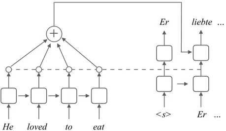
The most successful approach to machine translation is currently the attentional encoder-decoder model[KB13, SVL14, BCB15], which we will sometimes refer to simply asencoder-decoder modelfor brevity. These models are also called sequence-to-sequence models in literature. We describe this approach in detail because subsequent chapters will introduce extensions to it. Figure 2.1 illustrates the model architecture.

He loved to eat

+

<s> Er …

Er liebte …

Figure 2.1: Encoder-decoder model architecture.

We begin by factorizing the conditional probability as the product of conditional probabilities of each token to be generated:

p(y|x) = M Y

t=1

p(yt|y<t,x).

The training objective is to estimate parameters θ that maximize the log-likelihood of the sentence pairs in a given parallel training data setD:

J(θ) = X (x,y)∈D

(27)

2.1 Neural Machine Translation

2.1.1 Encoder

The encoder is a bi-directional recurrent neural network (RNN), following Bahdanau et al. [BCB15]. Here, the source sentence is processed in both the forward and backward directions with two separate RNNs. For every inputxi, two hidden states are generated as − → hi= LSTM Efwd(xi), − → hi−1 (2.1) ←− hi= LSTM Ebwd(xi), ←− hi+1 , (2.2)

whereEfwd and Ebwd are source embedding lookup tables. A typical choice of RNN is long short-term memory (LSTM) [HS97, Section 2.1.4] which has been demonstrated to achieve high accuracy in many situations. Multiple LSTM layers can be stacked, with bidirectional outputs concatenated either after every layer or only after the final layer. We obtain the final hidden encoder state hi =

− →

hi | ←−

hi, where layer indices are omitted for simplicity.

2.1.2 Attention

We use an attention mechanism [LPM15] to summarize the encoder outputs into a fixed-size representation. At each decoding time stepj, a context vectorcj is computed as a weighted average of the source hidden states:

cj = N X

i=1

αijhi.

The normalized attentional weights αij measure the relative importance of the source words for the current decoding step and are computed as a softmax with normalization factor Z summing overi:

αij = 1

Z exp s sj−1,hi

s(·) is a feed-forward neural network with a single layer that estimates the importance of source hidden statehi for producing the next target symbolyj, conditioned on the previous decoder statesj−1.

(28)

2. BACKGROUND

2.1.3 Decoder

The decoder generates output symbols one by one, conditioned on the encoder states via the attention mechanism. It uses another LSTM, initialized using the final encoder hidden state: s0 =hN. At decoding stepj, we compute

sj = LSTM Etrg(yj−1),sj−1

˜

sj = tanh(Whs[sj;cj] +bhs)

The conditional probability that thej-th target word is generated is:

p(yj |y<j,x) = softmax(Wso˜sj+bso).

Here,Etrgis the target embedding lookup table,Whs andWso are weight matrices, and

bhs and bso are bias vectors.

During decoding, beam search is used to find an output sequence with high conditional probability.

2.1.4 Long Short-Term Memory RNNs

At the heart of both the encoder and decoder are recurrent neural networks such as LSTMs [HS97]. These are computed as follows:

fi=σ(Wfxi+Ufhi−1+bf) forget gate (2.3) ii=σ(Winxi+Uinhi−1+bin) input gate (2.4) oi=σ(Woxi+Uohi−1+bo) output gate (2.5) ui= tanh (Wuxi+Uuhi−1+bu) update (2.6) ci=iiui+fici−1 cell (2.7) hi=oitanh(ci) hidden (2.8)

Inputs xi are embeddings or hidden states of a lower layer at timestep i, hi are the hidden states andci the cell states. W·and U· denote parameter matrices,b·bias terms. LSTMs mitigate the vanishing gradients problem of vanilla RNNs by using a gating mechanism in which sigmoidal gates explicitly control how much information in the cell state should be kept or overwritten [Hoc98].

(29)

2.1 Neural Machine Translation

2.1.5 RNN-Free Models

RNNs have proven powerful sequence models in many tasks, but also possess a practical drawback: Their slow computation speed. The reason for this is that computations across a sequence cannot be parallelized because the computation at each time step depends on the outcome at the previous time step. This has led researchers to consider alternatives to RNNs, the most popular ones being time-delay/convolutional neural networks (TDNNs/CNNs) and self-attentional neural networks.

TDNNs/CNNs have been proposed in the late 1980s [WHH+87, WHH+89] for acoustic modeling, and have also been extensively used in computer vision [LBD+89]. However, only relatively recently have they been applied to discrete sequence modeling [KGB14, Kim14, SHG+14] and machine translation [GAG+17]. These networks define learnable filters over receptive fields of a fixed and usually small size. By stacking multiple layers the receptive field grows larger in each layer. Parallelization on modern GPU hardware is possible because each time step can be computed independently of the other time steps.

A limitation of TDNNs/CNNs is that the context is still fixed to a window of a certain size, even after stacking multiple layers. This is in contrast to RNNs that condition on infinitely long contexts, at least in theory. Recently, self-attentional models have been introduced [CDL16, PTDU16, LFdS+17] that combine support for arbitrarily large contexts and parallelization. They have been found to yield excellent results for machine translation [VSP+17].

The main idea behind self-attention is to condition the state for every time step on every other time steps by computing pairwise relevance scores. The attention mechanism is used to compute such relevance scores and makes sure that weights for all states sum up to 1. The new state is then computed as the weighted average over all other states. Formally, let [x1. . .xl] denote a sequence of state vectors. For each positionxi,1≤i≤l, we compute the following:

eij =f(xi,xj) ∀l: 1≤j≤l (2.9) αi= softmax (ei) (2.10) yi= l X j=1 αijxj (2.11)

(30)

2. BACKGROUND

products, bilinear combination, or a multi-layer perceptron. f is used to establish relevance between all pairs of sequence items. These are then run through a softmax and used to compute a weighted average over all states, independently at each position. For sufficient model expressiveness, multiple layers can be stacked and interleaved with position-wise multi-layer perceptrons [VSP+17].

2.1.6 Modeling Units

Neural sequence models have traditionally used word tokens as modeling units [BDVJ03], based on the intuition that language is usually based on words to convey particular concepts, and on the idea of using word embeddings in continuous space to relate such word-based concepts to one another. This position can be challenged in several ways. First, some languages such as Chinese and Japanese have no clear concept of a word. Second, sparsity issues lead to poorly estimated word embeddings, particularly in languages with rich morphology or compounding. Third, these models cannot account for unseen words, a common problem even in languages without rich morphology.

An obvious alternative is to use characters as basic modeling unit. These form the basis of virtually every language that has a writing system, often do not suffer from sparsity issues, and can account for unknown words. In practice, character units require smaller embedding spaces and are much cheaper to compute at the softmax output projection. Despite this, they usually lead to more expensive models because sequence lengths are much longer, and sometimes larger hidden dimensions are required [BJM16]. Also, they often perform slightly worse than word-based models.

These trade-offs have led researchers to consider sub-word models, exploring the space between words and characters as units [MSD+12]. The currently most popular technique is byte-pair encoding [SHB16] which allows to flexibly choose a tradeoff between vocabulary size and sequence length.

Besides the issues mentioned above, there are two important factors in practice that determine whether characters, words, or sub-words are the most desirable representation. First, the data size: For small training data, sparsity issues can become severe and character-level models or small sub-word units often perform best, while for large data sets longer units are preferable. Second, when using an attention mechanism in an encoder-decoder model, it is desirable to have similar scales at both sides so that similarity scores are computed between comparable entities.

(31)

2.2 Automatic Speech Recognition

2.2

Automatic Speech Recognition

Hidden Markov model (HMM) have been explored in the 1970s for the recognition of continuous speech at IBM [JBM75] and Carnegie Mellon University [Bak75] and have provided the by far dominant framework for continuous speech recognition until very recently. As HMM-free, all-neural methods are achieving increasingly competitive accuracies in recent years, there is less clarity about what the best approach is compared to the translation scenario. All-neural methods include connectionist temporal classification [GMH13], attentional encoder-decoder models [CJLV16, BCS+16], and the recurrent neural aligner [SSRB17]. In this thesis we make use of both HMM-based and encoder decoder-based speech recognition and survey both below.

2.2.1 Preprocessing

Acoustic signals for speech are represented as discrete sequences of samples of the changing electric currents in a microphone. These samples are captured through an A/D converter at intervals of a certain frequency, often 16kHz, and quantized to e.g. 16-bit numbers. The resulting representation contains a large amount of numbers for every speech utterance, which is challenging for both computational and modeling reasons. The signal must therefore first be mapped to a space of much lower dimension while attempting to remove much of the redundancy present in a speech signal.

Based on the observation that humans can acquire the skill of interpreting speech signals in the frequency domain but are very poor at doing the same in the time domain, many preprocessing methods use the discrete Fourier transform to convert the signal into the frequency domain. This is done with windows of e.g. 16ms or 25ms size, chosen to be shorter than the length of most phonemes that occur in a signal. The windows are shifted by a step size of e.g. 10ms to capture the sequence of acoustic events. The feature space can be reduced by grouping the spectrum into bins that cover a certain range of frequencies each. To this end, the Mel scale can be used to divide into bins that correspond to perception by the human ear. The result is a feature representation called Mel filterbank features that will be the main technique used throughout this thesis. Other common techniques are cepstral coefficients that applies a series of further transformations, or perceptual linear prediction that follows a rather different predictive approach [RJ93].

(32)

2. BACKGROUND

2.2.2 HMM-based Speech Recognition

HMM-based speech recognition decomposes the task using the intuition of the noisy channel model [Sha48]:

ˆ W = argmax W P r(W|X) = argmax W P r(X|W)·P r(W) P r(X) = argmax W P r(X|W)·P r(W),

where W denotes a word sequence, X is an acoustic observation, and ˆW is our best guess for the true uttered word sequence. The noisy channel considers the correct word sequence as having been garbled by a noisy channel so that only a noisy signal is observed; the task is then to decode the original signal (the word sequence) based on the noisy signal (the acoustic signal). In the derived formula, P(W) is a linguistically motivated prior, and P(X|W) is the likelihood term, i.e. the probability of observing the acoustic sequence given a particular word sequence. The noisy channel model offers a convenient machinery for combining the prior and the conditional model.

Feature extraction Decoder Acoustic model Pronunciation dictionary Language model Acoustic

signal Output word sequence

Figure 2.2: Block diagram of HMM-based speech recognition.

Figure 2.2 illustrates how this approach is put to practice. The speech signal is preprocessed as outlined in Section 2.2.1 to obtain a sequence of feature vectors X. P(W) is usually computed by ann-gram language model [Sha48, CG98], andP(X|W) can be modeled through a GMM-HMM or hybrid acoustic model. Furthermore, because acoustic models work over phonemes but language models over words, a pronunciation dictionary is necessary to establish a proper mapping. Importantly, the language model, acoustic model, and dictionary are estimated independently of each other. Decoding is realized by employing a beam search over the hypothesis space. Because this model is often unable to handle punctuation and produces numbers and other special terms in a pronounced format that is hard to read, a post-processing step is necessary to produce legible output.

(33)

2.2 Automatic Speech Recognition

2.2.3 Encoder-Decoder-Based Speech Recognition

A drawback of the HMM-based approach is the need for creating pronunciation dictionaries, posing a considerable burden when developing ASR for new languages. A recent trend has therefore been to learn dictionaries implicitly via neural methods, often referred to as end-to-end ASR. One common approach is connectionist temporal classification (CTC) [GMH13] which computes a high-level representation of a sequence of acoustic feature vectors using an RNN, and then classifies each frame by assigning it e.g. an alphabet letter in the case of English. Blank labels and mechanisms to deal with repeated characters are used to account for the fact that the input sequences are much longer than the output sequences, and the CTC loss function marginalizes over all equivalent outputs (also called segmentations) via a dynamic programming approach.

CTC eliminates the need to create dictionaries, but is still dependent on external language models for good performance. This is because outputs are conditionally independent of each other, therefore only a weak implicit language model can be learned in the RNN layers. A remedy to this is provided by the listen-attend-spell model [CJLV16], another HMM-free approach to speech recognition that uses an encoder-decoder architecture as described in Section 2.1 with a few modifications.

The learned word embeddings are replaced by acoustic features (see Section 2.2.2), such that the encoder component now serves as an acoustic model. Because acoustic sequences are very long compared to text inputs, the encoder performs downsampling to make memory and computation time manageable. This is achieved through a pyramidal LSTM, a stack of LSTM layers where pairs of consecutive outputs of a layer are concatenated before being fed to the next layer, such that the number of states is halved between layers. As output units, characters rather than words are used and yield much better results. This can be explained by a more direct correspondence between encoded units (downsampled audio frames) and outputs, and by the fact that training data in number of words is usually much smaller for speech recognition than machine translation, causing data sparsity problems when using full word-based vocabularies.

Note several important differences to the HMM-based approach:

• No noisy-channel assumption is made. Instead, P(W |X) is modeled directly.

• All parameters are trained jointly. This can be a desirable property and can also simplify implementation and maintenance. On the other hand, exploiting auxiliary data such as monolingual data for language modeling becomes less straight-forward.

(34)

2. BACKGROUND

• No pronunciation dictionary is required, the creation of which is one of the major burdens in traditional speech recognition.

• This model is more flexible regarding output text normalization, e.g. can be trained to directly produce output that is properly cased, punctuated, and uses properly formatted numbers.

2.3

Considerations for Cascaded Systems

Even in the hypothetical case of a perfect speech recognition system, simply chaining the aforementioned speech recognition and machine translation models as-is would be problematic because the speech recognition output differs from the machine translation training data in significant ways. Such train-test mismatch is a reason of degradation with many machine learning models. The most important problems are listed below. Not all of these are dealt with explicitly in this thesis, but a good understanding is nevertheless important. Section 2.4 will survey the proposed solutions in existing literature.

2.3.1 Text Normalization

Speech recognition output is often unpunctuated, contains numbers as written-out words, and may otherwise differ regarding normalization conventions. Therefore, the speech recognition output must be post-processed to follow conventions of the translation training data as closely as possible in order to minimize the data mismatch and avoid out-of-vocabulary problems.

2.3.2 Segmentation

In scenarios where the input is either a very long audio, or comes as a live stream of unbounded length, speech recognition outputs may be unsegmented or possess segmentation guided by acoustic properties rather than into linguistically meaningful sentences. This is in contrast to the translation training data that usually consists of well-formed individual sentences. In addition to the mismatch, reordering phenomena often make it necessary to be in possession of a full sentence in order to translate it. Therefore, a segmentation step must be performed, often jointly with the punctuation step needed for text normalization. When doing simultaneous translation this is further complicated by the lack of future context, and often one must trade off between high translation accuracy and low latency.

(35)

2.4 Speech Translation: Prior Research

2.3.3 Style

Spoken language is often more casual, less grammatical, and may suffer from disfluencies such as false starts, repetitions and filler words. It uses a limited vocabulary, makes many inexplicit references, and is structured as shorter intonation units that are often not topically coherent [CD87]. None of these phenomena are likely to be appropriately captured by the textual translation training data. It can therefore be beneficial to remove disfluencies and correct incorrect grammar before attempting translation. Note that the style mismatch can be of varying degrees. For example, a well-rehearsed lecture is usually closer in style to written language than a spontaneous dialog between family members.

2.3.4 Paralinguistic Information

Spoken representations of text often do not represent paralinguistic information such as word emphasis. However, such information can be very useful for translation purposes, especially when generating speech outputs, but also for text outputs. Some prior work approaches this issue by including emphasis information into the ASR output and proposing ways for translating such representations [DSN18, KTS+13, AOB12, AAB06, TGN13].

2.4

Speech Translation: Prior Research

2.4.1 Early Work

Early efforts to speech translation around the Janus project [WJM+91, WCE+93, LGG+95] used a simple cascading approach where speech recognizer and translation systems were built separately and the best hypothesis of the former would be used as input to the latter. Another early approach used template matching for the translation stage [WW91]. The possibility of speech-to-speech translation, producing speech output instead of text output, has also been considered, for example by Lavie et al. [LGG+95]. However, whether to output text or speech has usually been treated as a user interface issue that should be evaluated separately and can be achieved by simply applying speech synthesis to the speech translation text outputs. These early efforts were focused on limited domains such as a scheduling dialog scenario, in which results were promising. However, errors propagated from the speech recognizer were especially challenging for interlingua-based machine translation, widespread at this time, because it relied on parsers that in turn often expected well-formed inputs [WCE+93, LGG+95, LGGP03].

(36)

2. BACKGROUND

Along with the trend in general machine translation, following work turned increasingly to data-driven approaches [WW98, TMS+98, BBF+02, SSN07].

2.4.2 Integration of Components

Research efforts soon turned to the question of how to better integrate the recognition and translation stage. Ney describes a probabilistic framework for fully integrated data-driven approaches [Ney99]. According to this framework, speech translation seeks a solution to argmax eI 1 P r eI₁ |xT₁ , or equivalently to argmax eI 1 P r eI₁P r xT₁ |eI₁,

where eI₁ are the translated words in the target sentence of length I, and xT₁ are the frames in the acoustic sequence of lengthT. While the speech transcriptf₁J is ultimately of no interest to us,1we can bring it into the model by marginalizing over all possibilities:

argmax eI 1 P r eI₁P r xT₁ |eI₁= argmax eI 1 P r eI₁ X fJ 1 P r f₁J |eI₁P r xT₁ |f₁J

Explicit marginalization is intractable, efforts can therefore be categorized by the approximations they take.

A first simple way of better integrated recognition and translation is moving from 1-best translation to n-best translation. This option was explored by Quan et al. [QFC05] and Lee et al. [LLL07], but has been mentioned in earlier works as well [LGG+95]. The n-best approach corresponds to replacing the sum over all possible transcriptsf₁J by a sum over only the list of then-best outputs of the speech recognizer. This was found to improve results in the travel domain while being rather expensive.

On the opposite end of the spectrum was a fully integrated approach that used the finite state transducer (FST) formalism to model a decoder that directly produced translations from audio inputs, with corresponding transcript as a side product [Vid97, BR01, CNO+_{04, PGJ}+_{07]. Conveniently, this approach allowed using} general-purpose FST tools to conduct an approximate search over the intractable search

1_{One may argue that this is not always true: Speech translation user interfaces often display both}

the transcript and the translation to the user, making it necessary to produce not only a translation but also a transcript.

(37)

2.4 Speech Translation: Prior Research

space. Conceptually, this amounted to permitting the full marginalization in the model, but exploring only a limited region of the search space by using pruning and other search heuristics. Results were promising in a limited domain scenario, hotel front desk dialogs, but also somewhat inconsistent and revealed robustness issues.

Follow-up work suggested using word graphs such as lattices [SJVS04, ZKYL05] or confusion networks [BF05] as a more compact and computationally convenient alternative to n-best lists. Word graphs integrated nicely with word-based translation models based on the IBM models [BPPM93]. While slight improvements were observed in some cases, the main advantages turned out to be of computational nature. After phrase-based translation [KOM03] emerged, Matusov et al. developed a method for performing lattice decoding in a phrase-based context and reported good results [MNS05, MHN08]. Evaluated speech translation tasks were now moving from limited travel-related tasks to open-domain tasks such as translation of TED talks [TED12] or speeches from the European parliament.

2.4.3 Advanced Topics

With accuracies of even the cascaded approaches reaching more acceptable levels, researchers turned to tackle the more advanced aspects of speech translation (see Section 2.3). Domain adaptation techniques were used to adapt models to the spoken language domain [LGGP03, Füg08]. It was shown how to automatically optimize recognition outputs that lead to better translation quality [KBT+15, HDA11]. The scenario of translating longer speeches rather than short utterances was explored. This scenario is challenging because machine translation models can usually handle only single sentences, but sentences boundaries are unknown. The works by Matusov et al. [MMN06] and by Fügen [Füg08] thus segment the speech recognition output and insert punctuation to optimize translation performance. As such systems are often deployed in a real-time situation, simultaneous speech translation with low latency is a very useful feature [Füg08, ONS+14, NPH+18]. As spoken language contains disfluencies that hurt readability of the transcript and causes translation errors, disfluency removal [CFH+_{13] can be beneficial.}

2.4.4 Speech Translation Corpora

It is important to realize that all efforts to this point had used separate speech recognition and machine translation translation corpora to train models. Translated speech data was only available in small quantities and was useful only as validation

(38)

2. BACKGROUND

and test data, but not for training. This often led to domain mismatch between the translation and recognition components, and it was recognized that addressing this issue would also result in a tighter integration of both models. One approach was to generate synthetic speech recognition outputs by imagining recognition errors, which can then be used to train a more robust translation model [TMD14, RGLF15]. Some efforts were devoted to collecting speech translation corpora that could be used for training purposes [SKM+12, PKL+13, GAAD+18, KBK18]. However, initial attempts by Post et a. did not observe gains from training a machine translation model directly on speech recognition output [PKL+13]. Paulik made use of interpreted speech data, i.e. speech utterances paired with the utterances of a human interpreter [Pau10]. Such data can be easier to obtain in some situations, but is a less direct form of supervision for a speech-to-text translation system.

2.4.5 New Chances and Challenges

Machine translation and speech recognition, as well as machine learning in general, underwent several major changes in the past years and decades. Machine translation transitioned from interlingua-based approaches to statistical approach and then to end-to-end trainable neural approaches in recent years. Speech recognition has long been dominated by HMM-based models, but these have recently been challenged (though not replaced) by end-to-end trainable neural approaches. These changes re-raise some of the questions and issues related to speech translation. For example, it has been observed that neural machine translation is less robust to speech recognition errors than statistical machine translation models, although overall accuracies are improved enough to make up for this [RDBF17]. Prior approaches to lattice translation are no longer applicable with neural machine translation because output independence assumptions no longer hold. Finally, the question of how to leverage end-to-end speech translation corpora has not been conclusively answered.

(39)

Chapter 3

Databases

This chapter introduces two speech recognition corpora and one speech translation corpus that will be used throughout this thesis. The chapter is then concluded by discussing evaluation metrics that can be used to assess model performance based on the given data.

3.1

WSJ

The Wallstreet Journal (WSJ) continuous speech recognition corpus [PB92] contains English sentences selected from the Wallstreet Journal and read by a variety of speakers. It is a widely used benchmark in speech recognition. The speech being read instead of spontaneous places this corpus is on the easier side of the spectrum. Table 3.1 shows statistics of this corpus, and Table 3.2 lists some examples. We will make use of it to develop our speech recognition baseline in Section 4.1.

Data set Audio duration Number of utterances Number of words

WSJ/Train (I284) 81h 37,416 645,876

WSJ/Dev (dev93) 1:05h 503 8,334

WSJ/Test (eval92) 0:42h 333 5,700

(40)

3. DATABASES

1 he chats with her briefly then resumes his political analysis

2 quote we have a dirty war exactly the same as in argentina unquote he says

3 quote it isn’t acceptable but it’s understandable unquote noise

4 and what should the government do about the murders

5 nothing says the businessman

Table 3.2: WSJ corpus example utterances. A curiosity are the explicitly spoken punctuation marks.

3.2

TEDLIUM

The TEDLIUM corpus [RDE14] is a widely used corpus of recorded TED talks [TED12], containing talks on technology, entertainment, and design, delivered in English by well-prepared, high-profile speakers. The corpus includes the recorded audios and transcripts created by volunteers. In this thesis, we use its second edition. Compared to WSJ this is a more difficult speech recognition task because it contains realistic, spontaneous speech. However, the level of difficulty is still only moderate because the audio quality is excellent and the preparedness of the speakers results in only a limited amount of disfluencies and other characteristics of spontaneous speech. Table 3.3 shows the statistics, and Table 3.4 lists example utterances.

Data set Audio duration Number of utterances Number of words

TEDLIUM/Train 206h 92,968 2,250,412

TEDLIUM/Dev 1:35h 507 18,226

TEDLIUM/Test 2:37h 1,157 28,432

Table 3.3: TEDLIUM corpus statistics.

1 and now we ’re trying to go from that digital code

2 into a new phase of biology with designing and synthesizing life so we ’ve always been trying to ask big questions

3 what is life is something that i think many biologists have been trying to understand at various levels we ’ve tried various approaches

4 paring it down to minimal components we ’ve been digitizing it now for almost twenty years when we sequenced the human genome it was going from the analog world of biology into the digital world of the computer

5 now we ’re trying to ask can we regenerate life

(41)

3.3 Fisher-Callhome

Audio duration Number of sentences Number of words

Fisher/Train 162h 138,819 1,810,385 Fisher/Dev 4:21h 3,979 50,700 Fisher/Dev2 4:28h 3,961 47,946 Fisher/Test 4:14h 3,641 47,896 Callhome/Train 13h 15,080 181,311 Callhome/Devtest 3:33h 3,966 47,045 Callhome/Evltest 1:47h 1,829 23,626

Table 3.5: Fisher-Callhome corpus statistics.

1-best WER Lattice oracle WER

Fisher/Dev 41.3 19.3

Fisher/Dev2 40.0 19.4

Fisher/Test 36.5 16.1

Callhome/Devtest 64.7 36.4

Callhome/Evltest 65.3 37.9

Table 3.6: Accuracy of ASR outputs in Fisher-Callhome corpus.

3.3

Fisher-Callhome

We conduct most of our speech translation experiments on the Fisher and Callhome Spanish–English Speech Translation Corpus [PKL+13]. This is a corpus of Spanish telephone conversations that includes audio recordings, transcripts, and translations into English, as well as automatic transcripts and speech recognition lattices created by a Kaldi system. The Fisher portion consists of telephone conversations between strangers, while the Callhome portion contains telephone conversations between relatives or friends. Data statistics are shown in Table 3.5. For the Fisher development and test sentences, four translation references exist, while for sentences from Fisher/Train and Callhome there is only a single reference translation. ASR word error rates (WER) are relatively high (Table 3.6), due to the spontaneous speaking style and challenging acoustic conditions. From a translation viewpoint, on the other hand, the data can be considered as relatively easy with regards to both the topical domain and particular language pair. Table 3.7 lists some example utterances with their translations. Lattices contain on average 3.4 (Fisher/Train) or 4.5 (Callhome/Train) times more words than their corresponding reference transcripts. The average sentence length is between 11.8 and 13.1.

(42)

3. DATABASES

Source sentence Translated sentence

1 al´o hello

2 al´o hello

3 hola hello

4 hola hello

5 con qui´en hablo with whom am i speaking

6 eh silvia s´ı c´omo se llama eh silvia yes what is your name

7 hola silvia eh yo me llamo nicole hello silvia eh my name is nicole

8 ah mucho gusto ah nice to meet you

9 mucho gusto em y d´onde est´a usted nice to meet you em and where are you from

10 n eh yo estoy en filadelfia eh i’m in philadelphia

11 ay mira yo estoy en nueva york aye look i’m in new york

12 y ust ah no sab´ıa que el estudio and you ah i didn’t know that the study inclu´ıa gente tan lejos pero que bueno included people so far but how nice

13 s´ı yo particip´e en un es un estudio yes i participated in a study like this as´ı em hace como un a˜no y em like a year ago and

14 ah ah mm mi hijo particip´o en ese s´ı ah ah hmm my son participated in this yes

15 s´ı supe que es para todo pa´ıs o yes i knew that it was in the whole country sea para gente de todo pa´ıs like people from the whole country

Table 3.7: Fisher corpus example utterances.

3.4

Evaluation

Throughout this thesis we mainly rely on automatic reference-based evaluation to assess accuracy and compare different models. The main metrics we use are word error rate (WER) for speech recognition and BLEU (short for bilingual evaluation understudy) for translation.

3.4.1 WER

WER is based on the edit distance, also referred to as Levenshtein distance. The main idea is to count the minimum number of word-level edits necessary to transform the incorrect output string into the correct reference string. Edits can be substitutions, insertions, and deletions. The WER is then defined as

WER = substitutions + insertions + deletions

reference length ×100%.

The minimum number of edits can be computed efficiently through a dynamic programming algorithm. In languages where no clear word boundaries exist, such as

(43)

3.4 Evaluation

Chinese and Japanese, the character edit rate can be used instead which works exactly the same but operates on character-level instead of word-level.

While WER is meaningful even when computed for individual test sentences, it is usually computed at the corpus level, so that longer sentences in the corpus are given proportionally more weight in the final score than shorter sentences.

3.4.2 BLEU

The BLEU score [PRWZ02] is based on a precision term that computes how many n-grams in an output actually appear in the reference string, and a brevity penalty that prevents gaming the metric by generating short translations that contain only safe or highly confident n-grams:

BLEU4 = brevity penalty× 4 Y i=1 precision_i, where precision_i= P

ngram∈outputCountclip(ngram) P

ngram0_∈_outputCount (ngram0)

.

Commonly, precision scores for n-grams up to order 4 are computed, as shown in the equation. Countclip(ngram) refers to a clipped count, i.e. the number of output

n-grams that appear in the reference where eachn-gram in the reference can be used only once.

The brevity penalty is defined as follows:

brevity penalty = min(1, e1−reference lengthoutput length ₎_.

BLEU scores can also be computed against multiple references, in which case the clipped counts are clipped at the maximum count of n-grams which occurs in a single reference, and the brevity penalty is computed against the length of the reference closest in size to the candidate translation.

Note that then-gram precision for higher ordern-grams, e.g. 4-grams, is not unlikely to be zero for a single sentence, which would result in the BLEU score for a whole sentence becoming zero. For this reason, BLEU-scores are computed at the corpus level, not at the level of individual sentences.

(44)

(45)

Chapter 4

All-Neural Speech Recognition

As a first step toward advancing speech translation using recent deep learning techniques, we first experiment with a speech recognition task. Speech recognition can be seen as an easier version (or subtask) of the speech translation task, with acoustic modeling similarly challenging but without the complexities of having to produce outputs in a different language. This makes speech recognition an ideal test bed for improving models, debugging implementations, and conducting analyses. A good speech recognition model can also directly improve speech translation by helping form a strong cascade. This chapter first describes efforts to produce and analyze a strong baseline based on state-of-the-art modeling techniques from the available literature, and then explores novel improvements. Importantly, this chapter directly modelsP(W |X), the probability of the transcript W given the audio signalX, with no decompositions. This will allow us in Chapter 6 to extend the models introduced here to be capable of

translating speech.

4.1

Analyzing the State of the Art

We start by describing the development of a strong baseline system by using the initial work by Chan et al. [CJLV16] as a starting point. This work has formed the basis of many subsequent works on attentional speech recognition models and has been reported to yield promising results competitive with other models.

4.1.1 Basic Settings

We choose basic settings based on findings in literature and on our own preliminary experiments. These settings are used throughout the thesis unless otherwise noted.

(46)

4. ALL-NEURAL SPEECH RECOGNITION

For audio preprocessing, we extract 40-dimensional Mel filterbank features with per-speaker mean and variance normalization. We exclude utterances longer than 1500 frames from training to keep memory requirements manageable. The encoder-decoder attention is MLP-based, and the decoder uses a single LSTM layer. The number of hidden units is 128 for the encoder-decoder attention MLP, 64 for target character embeddings, and 512 elsewhere unless otherwise noted. The model uses input feeding [LPM15]. For the encoder, we use bidirectional LSTMs with 256 hidden units per direction. During inference, we use beam search and length normalization.

We set the batch size dynamically based on the number of source and target tokens of the longest sentence in the minibatch. We choose the average batch size such that most of the available GPU memory is used, here 24 utterances per minibatch. We use Adam [KB14] with initial learning rate of 0.0003, decayed by 0.5 when validation WER did not improve over 10 epochs initially and 5 epochs after the first decay. We implement our method based on the DyNet neural network toolkit [NDG+17].

4.1.2 Findings

We start our exploration using a vanilla implementation of the listen-attend-spell architecture by Chan et a. [CJLV16] that features a pyramidal LSTM encoder and the settings just described.

Overfitting. Overfitting is a major challenge in attentional speech recognition and proper generalization techniques are therefore an important consideration. While prior work has often used weight noise and weight decay for normalization, we have observed inconsistent gains and a necessity to perform expensive grid search to tune the respective hyperparameters. Instead, we opt for a solution that uses variational dropout combined with target character type dropout, both proposed by Gal et al. [GG16], both because it yielded best results and because it was more stable across the various models and settings.

In particular, recurrent dropout is applied to all LSTMs that are used in the encoder or decoder. Independently for each LSTM layer, direction, and minibatch element, we draw dropout masks mx and mh from a multivariate Bernoulli distribution: mx ∼ Bernoullidx(1−p) and mh ∼ Bernoullidh(1−p) where p

it the dropout probability. We then replace hi−1 by ₁−1pmh hi−1 and xi by 1

(47)

4.1 Analyzing the State of the Art fi =σ Wf 1 1−pmxxi+Uf 1 1−pmhhi−1+bf forget gate (4.1) ii =σ Win 1 1−pmxxi+Uin 1 1−pmhhi−1+bin input gate (4.2) oi =σ Wo 1 1−pmxxi+Uo 1 1−pmhhi−1+bo output gate (4.3) ui = tanh Wu 1 1−pmxxi+Uu 1 1−pmhhi−1+bu update (4.4) (4.5)

Crucially, the same mask is applied at every time step, and only at training time but not at test time. For word type dropout, we randomly choose a fraction p of the word types from the vocabulary and replace all corresponding word embeddings by a zero-vector during training. More details are given in [GG16].

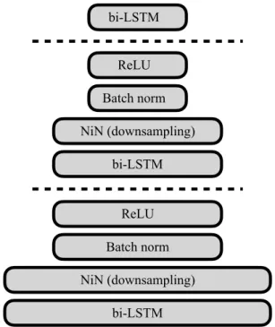
Encoder architecture. We implemented and tested several of the advanced encoder architectures proposed by Zhang et al. [ZCJ17]. While some of their models, in particular those that feature convolutional networks or convolutional LSTMs, did not yield improvements over our baseline, we did obtain good results using an LSTM/network-in-network architecture that stacks blocks consisting of a bidirectional LSTM, a network-in-network (NiN) projection, batch normalization [IS15], and a rectified linear unit (Figure 4.1). The final LSTM/NiN block is topped off by another bidirectional LSTM layer. NiN denotes a simple linear projection applied at every time step, possibly performing downsampling by concatenating pairs of adjacent projection inputs.

Label smoothing. Label smoothing has been found to prevent overconfidence and to improve decoding accuracy by Chorowski et al. [CJ17]. While the authors suggest a variant that smoothes across labels of adjacent time steps, we have found the simpler approach of uniform label smoothing [SVI+16] to yield best results. Specifically, instead of assigning all probability mass to the correct label at a particular decoding time step, we only assign it a probability ofβ, and spread the remaining probability mass 1−β uniformly over all remaining labels. Fixed embedding norm. In the context of neural machine translation, Nguyen et al.

suggest fixing the norm of target embeddings to a fixed value in order to prevent bias toward common tokens [NC18]. We confirm consistent improvements in the

(48)

4. ALL-NEURAL SPEECH RECOGNITION NiN (downsampling) bi-LSTM Batch norm ReLU NiN (downsampling) b