1 23
Public Transport Planning and Operations ISSN 1866-749X
Public Transp
DOI 10.1007/s12469-020-00249-7
Public transport network optimisation in
PTV Visum using selection hyper-heuristics
Philipp Heyken Soares, Leena Ahmed,
Yong Mao & Christine L Mumford
1 23
Commons Attribution license which allows
users to read, copy, distribute and make
derivative works, as long as the author of
the original work is cited. You may
self-archive this article on your own website, an
institutional repository or funder’s repository
and make it publicly available immediately.
ORIGINAL RESEARCH
Public transport network optimisation in PTV Visum using
selection hyper‑heuristics
Philipp Heyken Soares1 · Leena Ahmed2 · Yong Mao3 · Christine L Mumford2
Accepted: 18 August 2020 © The Author(s) 2020
Abstract
Despite the progress in the field of automatic public transport route optimisation in recent years, there exists a clear gap between the development of optimisation algorithms and their applications in real-world planning processes. In this study, we bridge this gap by developing an interface between the urban transit routing prob-lem (UTRP) and the professional transport modelling software PTV Visum. The interface manages the differences in data requirements between the two worlds of research and allows the optimisation of public transport lines in Visum network models. This is demonstrated with the application of selection hyper-heuristics on two network models representing real-world urban areas. The optimisation objec-tives include the passengers’ average travel time and operators’ costs. Furthermore, we show how our approach can be combined with a mode choice model to opti-mise the use of public transport in relation to other modes. This feature is applied in a special optimisation experiment to reduce the number of private vehicles on a selected set of links in the network. The results demonstrate the successful imple-mentation of our interface and the applied optimisation methods for a multi-modal public transport network.
Keywords Route optimisation · PTV Visum · Selection hyper-heuristics
* Philipp Heyken Soares
[email protected] Leena Ahmed [email protected] Yong Mao [email protected] Christine L Mumford [email protected]
1 Laboratory of Urban Sustainability, Nottingham University, Nottingham NG7 2RD, UK 2 School of Computer Science and Informatics, Cardiff University, Queen’s Buildings, The
Parade, Cardiff, UK
1 Introduction
Public transportation systems form an essential part of the infrastructure in urban areas. Their efficiency is vital to many stakeholders and, therefore, they require precise design and planning. The generation of efficient route networks for public transport systems is known in many studies as the urban transit routing problem (UTRP).1 This problem has been addressed in the literature by a considerable
num-ber of studies that vary in their application on different instances, objectives and solution methodologies.
Despite intensive research into the UTRP, there is a vast gap between the often purely academic studies and the application of their findings in real-world plan-ning processes. The reasons for the gap have not been thoroughly researched so far (Walter 2010). However, one possible explanation could be the differences in data requirements between the algorithms used in UTRP research and the commonly used planning tools. Planning agencies usually base their decisions on simulations made with professional transport modelling software, such as PTV’s Visum (PTV AG 2018) or INRO’s Emme (INRO 2018). Models built with software packages such as these require detailed information about the street layout, transport infra-structure, and travel demand, making them time-consuming to be implemented and calibrated. The resulting model, however, is very powerful and allows planners to study and simulate a variety of transport related phenomena. Researchers working on the UTRP on the other hand, apply their design algorithms to abstract models that simplify many aspects of real-world transport networks. A graph structure with interchange points as vertices and direct connections between them as undirected edges is the common model used by most previous studies.
In this work, we bridge the gap between the two worlds of theoretical research on the UTRP and real-world transportation planning. We focus here on Visum transportation modelling software and compare its transport network structure to a common UTRP model used previously by many researchers, pointing out the key differences between them. Based on these findings, we outline a process to trans-late Visum network components into the UTRP graph structure and vice versa by implementing a middle layer interface through which the transport network informa-tion passes between the models. Utilising this interface, selecinforma-tion hyper-heuristics are used to optimise Visum public transport routes while taking advantage of Visum analysis tools to evaluate a given candidate solution. The primary contributions of this study are:
1 The UTRP is, in fact, a sub-problem of a larger task to optimise public transport networks, which con-sists of five phases: (1) route design, (2) vehicles frequency setting, (3) timetables development, (4) vehi-cles scheduling and (5) crew scheduling (Ceder and Wilson 1986). As the phases are interconnected, the problem has very high complexity, and most studies only deal with subsets of these phases using simpli-fications. In the case of the UTRP, which only considers the first stage, a fixed frequency on all routes is assumed, and other aspects such as the actual departure and arrival times of vehicles at stop points are not considered.
– A comparative study of network structures used in the UTRP research and Visum, and a methodology for bridging between them.
– Novel interface procedures between Visum and the UTRP network models to facilitate transferring and translating data between them.
– Selection hyper-heuristic algorithm adapted to optimise Visum public transport routes utilising the interface procedures.
– The integration of Visum tools for the evaluation of candidate solutions.
The following sections are organised as follows: Sect. 2 outlines the historical back-ground of the UTRP in planning applications and provides a brief introduction to PTV Visum and its applications; Sect. 3 describes the UTRP and Visum network models in more detail; Sect. 4 summarises the interface processes; Sect. 5 outlines the optimisation procedure using selection hyper-heuristics and the applied evalua-tion tools. Finally, Sect. 6 presents our experimental results and Sect. 7 highlights the key findings and conclusion.
2 Background
2.1 A brief history of the UTRP
Attempts to automate the optimisation of urban public transport routes date back many decades using a variety of optimisation methodologies and algorithms. They generally fall into two categories: exact or heuristic-based methods. Exact mathe-matical approaches (Bussieck 1998; Chien and Schonfeld 1997; Guan et al. 2006; van Oudheusden et al. 1987) have been tested in many studies. The major limitation of such methods is the difficulty of finding optimal solutions in large-sized networks given the combinatorial nature of the problem, and this has resulted in their failure to scale up to practical sized instances.
Because of these shortcomings, research on the UTRP then shifted towards adopting heuristic-based methods to solve the problem, due to their ability to tackle large-size problem instances. Some heuristic methods are based on heuristic con-struction procedures, which attempt to build optimal public transport route sets from scratch. An example of such a method is the heuristic algorithm developed by Simonis (1981). This method starts by generating a route using the shortest path between the highest density demand points and then deletes the demand satisfied by this route. The process iterates to the next highest demand points until a maximal number of routes is reached. Other heuristic construction methods are described in (Baaj and Mahmassani 1995; Franz 1975; Silman 1974; Sonntag 1977).
The second group of heuristic methods attempts to improve a given input of route sets. These optimisation methods are usually based on meta-heuristic methods such as tabu search (e.g. Kılıç and Gök 2014; Pacheco et al. 2009), simulated annealing (e.g. Fan and Mumford 2010; Fan and Machemehl 2006) ant colony otimisation (e.g. Poorzahedy and Safari 2011; Yu et al. 2012), bee colony optimisation (e.g. Nikolić and Teodorović 2013, 2014), or genetic algorithms (GAs) (e.g. Heyken Soares et al.
sets are derived in some studies from the existing public transport network of the study areas. However, a heuristic construction procedure is often used to generate initial route sets. Examples of such a combination can be found in Ahmed et al. (2019), Heyken Soares et al. (2019), Kılıç and Gök (2014), and Mumford (2013).
Despite the huge amount of research on computer-based solutions for the UTRP, only few studies have been actually used in real-world planning processes (Walter
2010). One rare example is the work by Pacheco et al. (2009) which describes the optimisation of the bus network in Burgos, Spain, with regard to waiting times and trip duration. The solutions obtained improved significantly over those generated by planners of the city transport authorities using the same transit network data. Another example is a study 2012 by Cipriani et al. (2012) in cooperation with the mobility agency of Rome, Italy. It included the application of a genetic algorithm on an undirected graph representing the street network of Rome. The results show improvements over the existing bus route network in terms of waiting times, opera-tor costs and unsatisfied demand. According to the authors, the mobility agency of Rome had started implementing their results in 2012. Many other studies compare their results against the real existing routes, showing that their methods can lead to improvements over an existing service (e.g. see Ahmed et al. 2019; Bagloee and Ceder 2011; Bielli et al. 2002; Heyken Soares et al. 2019). However, the results of these studies have not been verified in real-world planning processes.
2.2 Interfacing UTRP algoirthms and transport modelling software
The key challenge for interfacing UTRP algorithms and macroscopic transport mod-elling software such as Visum or Emme, is to handle the differences between the undirected connections used in UTRP algorithms and the directed connections used in urban scale macroscopic modelling (more on this in Sect. 3).
All UTRP studies which have so far interfaced their algorithms with macroscopic transport modelling software have bypassed these problems by only using network representations with undirected connections. One such case is the mentioned above study on Rome (Cipriani et al. 2012), where the applied algorithm is interfaced with Emme. Other examples Alt and Weidmann (2011), and Bagloee and Ceder (2011) used Visum and Emme, respectively, and included procedures to construct suitable network representations.
So far, the most general tool for automatic public transport network optimisation in transport modelling software is the line proposal algorithm for Visum developed by PTV itself in 2006 (Nökel 2006). This tool applies a heuristic algorithm to an existing Visum network model. The algorithm first generates a palette of candidate routes between pre-selected stops. These candidate routes are then individually eval-uated in Visum and the route taking up the most demand is then permanently added to the network. This step can be repeated as often as required. The tool only requires a minimal interface as the algorithm simply controls the end points of routes and initiates their evaluation. All other aspects are handled by Visum and the algorithm does not modify the pre-existing routes. Although the algorithm has been success-fully used in at least two academic studies (Marauli 2011; Walter 2010), it remained
a prototype and was never fully developed into an official Visum extension. Unfortu-nately, it no longer works on recent versions of Visum.
2.3 Optimising public transport in Visum through selection hyper‑heuristics
The aim of this work is to create an interface between the UTRP network model and the macroscopic transport modelling software Visum, and utilise the interface to optimise Visum public transport routes using the general search methodology of selection hyper-heuristics.
Visum is a macroscopic transport modelling software package that combines both private (PrT) and public transport (PuT) into a single model and provides a rich suite of methodologies. It is a product of the PTV company based in Karlsruhe, Ger-many, and has been available for commercial use since the late 90s (Friedrich et al.
1999). It is used at present by transport planners and analysts throughout the world. The results presented in this paper have been produced using Visum 17, which was the latest released version at the start of this project.
In addition to the variety of analysis tools, one of the main reasons to use Visum for the present work is the ability to control it via Python scripts over the Visum COM-API (PTV AG 2014). This library provides a number of interface functions to control Visum via scripts and extract any required information. Such scripts form the basis of the present work.
Given the complexity of Visum software and its huge number of available fea-tures and tools, we have to limit the descriptions of its structure and capabilities to those which are vital for the present work. We will discuss the relevant data structures of Visum network models in Sect. 3.2 and the analysis options we use in Sect. 5.5. For further details we refer the interested reader to the Visum Manual (PTV AG 2018).
Selection hyper-heuristics are search methodologies motivated by the idea of generalising search techniques to several problem domains with minimal adaption. They have been applied to solve the UTRP for the first time in Ahmed et al. (2019). In this work thirty selection hyper-heuristics combining different combinations of selection and move acceptance methods with varying characteristics are tested on a set of known benchmark instances. A series of experiments and statistical com-parisons between the thirty methods revealed the success of an online selection method inspired by the hidden Markov model over other selection methods. Fur-thermore, the best performing algorithm was successful in finding single solutions of high quality in very short run times compared to the best published solutions. The same winning approach was applied in Ahmed et al. (2019) on a set of benchmark instances representing urban areas, and proved that it can surpass the performance of the genetic algorithm, NSGAII.
There are many advantages of a selection hyper-heuristic framework that makes it a good candidate for application on this work. First, it is a single point based frame-work, meaning it only requires a single initial solution. This allows us to extract the existing public transport network from a given Visum network model and use it as the initial solution. Second, maintaining a single solution while improving it
iteratively during the search, makes the interaction with Visum through the inter-face procedures straightforward. Also the relatively short run time of hyper-heuristic methods significantly adds to their attractiveness. A further description of the selec-tion hyper-heuristics framework is outlined in Sect. 5.
PuT: Refers to public transport. PrT: Refers to private transport.
G: Graph of connected vertices and edges. Used to represent a UTRP graph. v: Vertex of the UTRP graph belonging to the set of verticesV. Represents a stop in a Visum network model. (The terms stop and vertex can be used interchangeably in the UTRP graph.)
u: Terminal vertex (∈V), a vertex that routeris allowed to start and end with.
A: Adjacency matrix defines the connectivity of graphG.Ai,j=1 means a direct connection exists between vertexiand vertexj. In the case ofAi,j=0 the vertices are not directly connected.
r: Route in the UTRP graph as a path connecting a number of vertices. In Visum the route corresponds to a line. It is assumed to be bi-directional. s: Stop in Visum network. Represents a vertex in the UTRP Graph.
sp: Stop point in Visum network associated to exactly one stop. Can be used to define the course of the line route.
l: PuT line in Visum. The spatial course of the line is defined by its line routes.
lr: Line route in Visum. Belongs to exactly one line and specifies the spatial course of this line for one travel direction. Line routes are defined by stop points.
InfoBox 1: Summary of important concepts used in the following sections 3 Data structures
3.1 Defining the UTRP
Almost all previous approaches to the UTRP choose to represent the available street (or rail) network as a graph G= (V, E) . The vertices V = {v1, v2,…, v|V|} represent
access and interchange points, and the edges E= {e1, e2,…, e|E|} are direct
connec-tions between them. Using these definiconnec-tions, a PuT route r (e.g. a bus line) can be represented by a list of directly connected vertices. The route is usually assumed to be bi-directional, meaning that vehicles after completing a journey in one direction, can turn around and make the same journey in the opposite direction. For this to be
possible in an urban setup it is important that all routes begin and end at designated terminal vertices U= {u1, u2,…, u|U|} ∈V to allow U-turns. Following these
defi-nitions, the PuT network of a certain transportation mode can be described as a set of connected routes R= {r1, r2,…, r|R|} , which represents a solution to the UTRP
as an optimisation problem. This “route set” has to be connected, in such a way that each route has at least one vertex in common with one or more other routes in the route set.
In its simplest form, the structure of the graph G is given by an adjacency matrix
A|V|×|V| . This matrix defines the connectivity of the graph as follows: If two nodes
i and j are directly connected, the respective entry in the adjacency matrix equals
Ai,j =1 otherwise Ai,j=0 . This matrix must be symmetrical following the rule that
the routes are assumed bi-directional. The main advantage of such graphs for solv-ing the UTRP is that they allow constrainsolv-ing routes to be made up of only directly connected vertices. This excludes many possible flawed solutions and thereby drasti-cally reduces the search space.
Furthermore, information about the travel demand and the travel time between any two vertices in the graph is required for evaluation. This information is typi-cally provided in the form of two-dimensional matrices: the travel time matrix, and the demand matrix. Both matrices are usually symmetrical. The travel time matrix gives the travel time between directly connected vertices. Differences in travel times between directions (e.g. resulting from one way streets) are usually not considered. The demand matrix determines the number of travellers between any two demand sources. In the vast majority of studies, the vertices V are used as demand sources. Only about one in five studies use a zone demand structure similar to the structure used in macroscopic transport modelling (described below) (Heyken Soares 2020a).
3.2 Visum data structure
The inputs to Visum transport models also include travel demand and the network model of the available transport infrastructure.
As a standard practice in macroscopic transport simulations, the travel demand in Visum is aggregated at the level of zones ( Z= {z1, z2,…, z|Z|} ) and given in the
form of an origin-destination matrix. A demand matrix D|Z|x|Z| defines how many
trips are originating from zone zi , and travelling to zone zj . The demand data is given
as separate matrices for PuT and different modes of PrT (e.g. cars). However, it is possible to initially give the demand as one matrix aggregating all trips and then use a mode choice procedure to split the demand into separate matrices for different travel modes (more on this in Sect. 5.5.2).
The Visum network model is also based on a graph structure, though it is more detailed than the UTRP graph described above. Streets or rail segments are repre-sented by links usable for specified modes of transport. Links are composed of two separate network objects, one for each travel direction. Each one of these objects can have different attribute values such as the allowed speed, and capacity in terms of the number of vehicles. One-way streets can be represented by blocking one direc-tion of a link to all modes. Nodes at the beginning and end points of each link define
the positions of intersections and junctions in the network. Which turns are permit-ted for which mode at the represenpermit-ted junctions can be defined in the properties of the nodes. Each zone ( z∈Z ) must be connected to at least one node by a connector,
for exiting and entering the zone to the link network through this connection node. The Visum network model further includes other elements to represent the avail-able PuT lines and interchange points. PuT interchange points are defined in three layers. The “stop point” is the lowest layer indicating the actual stopping location of the vehicles (e.g. a segment of a train platform). Stop points can be placed either on nodes or links and can be used by all PuT lines traversing these network objects. A stop point placed on a link can either be accessible from both directions or can be restricted for use in a specific direction. The “stop area”, the middle layer, incorpo-rates one or more stop points (e.g. a platform on a train station). All the stop points of the same stop area are considered instantly connected while transfers between stop areas require a certain walking time. Further, a node can be allocated to a stop point area to allow access to the wider network model, most importantly to connec-tors connecting nodes to zones. The “stop”, the highest level, incorporates one or more connected stop areas (e.g. a train station) and is the level on which walking time between different stop areas is assigned. Stop areas do not play a major role in this work, and we will assume that stops and stop points are directly connected to simplify explanations.
PuT lines are also defined in several different layers. On the highest level is the “line”. Each line in Visum belongs to exactly one transport system. The spatial course of the line is defined by its line routes. A single line can aggregate several line routes that are defined by lists of stop points to be traversed in the given order.2
Line routes are thereby directed and most lines will have at least two line routes, one for each direction of travel. A special case are ring lines defined by single line routes starting and ending at the same stop point. Each line route is given a “time profile” describing, among other attributes, the travel times between the single stop points. “Vehicle journeys” with concrete departure times can be added to the line routes to create detailed timetables that specify departure and arrival times at the individual stop points.
3.3 Interfacing between the UTRP and Visum data structures
Based on the comparison of the standard graph structure of the UTRP with the respective data structure of Visum, there are key questions to be answered before constructing an interface between them. First we need to specify whether the opti-misation is going to be performed on the level of line routes or lines. Optimising the line routes individually can lead to significant deviations between the line routes that belong to the same line. This would not be desirable in practice. Therefore, we have chosen to perform the optimisation at the level of lines.
2 Technically the list defining a line route contains both stop points and nodes. However, it is sufficient to only provide the stop points as Visum can add the required nodes automatically via the shortest path search.
The second question is whether the vertices of the UTRP graph should represent stops or stop points in the Visum network model. To answer this question we need to consider that some stop points in the Visum network model might be restricted for use in specific directions only. This would conflict with the fact that routes in the UTRP structure are assumed bi-directional. However, in the majority of such
Fig. 1 a Schematic street network with one bus service (purple) and its stop locations (purple dots). b Representation of a as a Visum network model. Shown are links (black arrows) and nodes (blue dots), as well as stop points (triangles) and their stops (green circles) The stop points C and D are both part of stop 3. c UTRP graph with the stops in b as vertices and the possible direct connections between them as edges. d Sche-matic display of two line routes in the same network model as b representing the bus service shown in (a). The path of a line route is only defined by the stop points, although routing takes place along the nodes and links of the underlying network model with all the restrictions defined on it. Together both line routes form one line. e The line routes from d as a bi-directional list of vertices in the UTRP graph
(a)
(b) (c)
cases,3 the stops which these directed stop points belong to also incorporate other
stop points that are accessible from several directions (see Sect. 3.2 and Fig. 1). We, therefore, decided that the UTRP graph vertices should represent stops in the Visum network model rather than stop points.
Finally, it has to be decided which stops (i.e. vertices) should be considered as terminal vertices in the UTRP graph. It is recommended in PTV AG (2018) to exclusively use stop points that are placed on nodes as the beginning or end points of line routes. However, there are many existing line routes in the network models we used that do not follow this recommendation. We, therefore, select as terminal vertices, the stops which fulfil at least one of the following conditions:4 (a) Having
at least one of their stop points placed on a node. (b) Having at least one of their stop points being the beginning or end of an existing line route.
4 The interface processes
Based on the discussion in Sect. 3.2, we can formulate two main interface processes to translate routing information between UTRP algorithms and Visum. The first is to extract the adjacency relations between stops to be used as the basis for route alterations during the optimisation. This process will be introduced in Sect. 4.1. The second is a process to convert the modified routes (i.e. undirected lists of stops) into pairs of line routes (i.e. directed lists of stop points) to allow the implementation in Visum for evaluation. This process will be outlined in Sect. 4.2. The outcomes of both interface procedures are mode-specific, as some links in a Visum network model may only be accessible to specific modes.
4.1 Extracting a UTRP graph from a Visum network model
The process to extract the adjacency relations between the stops for a PuT mode m
from a given Visum network model is outlined in Algorithm 1. It begins by creating a stop point connectivity matrix Cm . This matrix has three types of entries: Cmi,j=0
indicates that there is no connection between the two stop points i and j, Cm i,j=1
means a direct connection between stop points i and j exists, and Ci,jm=0.5 indicates
that a connection exists but it is indirect (i.e. the connection goes over other stop points). Additionally, a distance matrix 𝛥m which records the travel time between
each pair of stop points is also created in this process (its usage is described in Sect. 4.2).
3 There are cases where a stop can only be reached from one direction. However, in all the networks examined in this work, these cases were very few in number and did not seem to have a significant impact on the results. We, therefore, neglected them at the present stage of the work. For the future, we plan to implement additional procedures that adequately address this problem.
4 The conditions listed here were selected for the optimisation of bus lines described in Sect. 6. For other scenarios or in case of optimising other PuT modes it might be necessary to adapt these conditions. Also, a manual selection of terminal vertices is possible.
Algorithm 1:Algorithm to generate the stop point connectivity matrix and distance matrix for a modemin a given Visum network.
Data: Visum Network
Result: Connectivity MatrixCm, Distance Matrix∆m 1 begin
2 for each Stop point i in Visum network do 3 for each Stop point j in Visum network do
4 Build test line routelof the modembetweeniand j.
5 ifl can be builtthen
6 ∆i,mj←travel time betweeniand j
7 n←number of stop points inl
8 ifn=2 then 9 Ci,mj = 1 10 else 11 Ci,mj = 0.5 12 else 13 Ci,mj = 0
14 return Cm,∆m, Visum network back to initial state.
A python script utilising functions from Visum COM-API is used to extract the required information from the given Visum network model. This script is demon-strated by Algorithm 1. For every possible combination of stop points i, j, the algo-rithm attempts to build a test line route beginning at i and ending at j by finding the shortest path along the links open to mode m. The building is only successful if Visum manages to find a shortest path from i to j considering all the constraints of the given network model. All other stop points located on this path are automatically connected to the built line route. If the test line route contains more than two stop points (not only i and j), the connection between i and j is considered indirect and recorded in the connectivity matrix as Ci,jm=0.5 . If no further stop points are
con-nected to the test line route, the connection is considered direct and recorded as
Cmi,j=1 . In either case, the travel time of the built line route is calculated by Visum,
and recorded in the distance matrix as 𝛥m
i,j . If the process of finding the shortest path
between i and j fails, these stop points are considered as not connected ( Cmi,j =0 ).
Once the algorithm has iterated through all stop point pairs, the Visum network model is returned to its initial state.
After the stop points connectivity matrix Cm is constructed, the adjacency matrix
Am
|V|×|V| of the undirected UTRP graph is built using the following rules: two stops X
and Y are considered connected ( Am
X,Y =AY,X=1 ) if and only if at least one stop
point x belonging to stop X is directly connected to at least one stop point y∗
belong-ing to stop Y ( Cm
x,y∗=1 ), and at least one stop point y belonging to stop Y is
indi-rectly connected to at least one stop point x∗ belonging to stop X ( Cm
other case, even if all stop points of the two stops X and Y are indirectly connected,
X and Y are considered as not adjacent ( AmX,Y =AmY,X=0). 4.2 Transforming UTRP routes to Visum line routes
During the optimisation process, the changed routes have to be implemented into Visum for evaluation. To do so, the lists of vertices (i.e. stops) in these routes need to be converted into two lists of stop points, one for each direction of travelling.5
As described in Sect. 3, a single stop can have multiple stop points. Therefore, the correct combination of stop points that represent a specific combination of vertices has to be selected. This is done with the help of a conversion table 𝛶m . Its use is
illustrated in Fig. 2.
Let us assume we have a route ri that contains the following set of vertices in
this order: {1, 2, 3, 4, 5} and vertices 2 and 4 are associated with multiple stop points
as illustrated in Fig. 2. To convert the route ri to a stop point list, we need to select
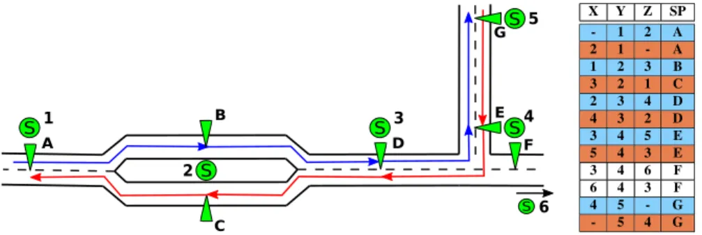
the correct combination of stop points that represent a particular direction of travel through a vertex. For the vertices associated with a single stop point this selection is trivial. However, for the vertices associated with multiple stop points, the selection process depends on the adjacent vertices and the order of these vertices in the route. In the example given in Fig. 2, the stop point representing stop 2 can be either B (if the order is 1, 2, 3) or C (if the order is 3, 2, 1).
The conversion table 𝛶m used to select the correct stop points for every vertex
is shown in Fig. 2. The first three columns give the possible triple set of connected vertices, one combination in each row. Every combination is considered twice, once for each travel direction. The fourth column specifies the stop point choice for the
Fig. 2 Schematic street network with five stops (1–5) and seven stop points (A to G). A sixth stop is
assumed along the street to the right. The UTRP route [1, 2, 3, 4, 5] is converted into two stop points lists using the conversion table on the right. The conversion table gives the correct stop point for a single stop using a combination of three stops (i.e. vertices) containing this stop and its adjacent stops. The resulting stop points lists are displayed in blue (from A, over B to D, E and G) and red (from G, E and D over C to A). For the terminal nodes, 1 and 5, a vertices triple with empty fields is given to be used at the begin-ning and end of a route, respectively
middle vertex in the combination. For terminals, additional triple sets with empty fields are used to determine the stop points at the beginning and end of a line route.
With the conversion done, the stop point lists can be implemented in Visum, replacing the old line routes by using Visum COM-API (PTV AG 2014). To allow PuT assignments to be run for the evaluation (see Sect. 5.5), time profiles and vehi-cle journeys can be generated as well.
The process to construct the conversion table 𝛶m is outlined in Algorithm 2. It
builds on data produced during the generation of Am (Algorithm 1), specifically the
connectivity matrix Cm and the distance matrix 𝛥m . For every vertex Y, the algorithm
identifies the vertices K adjacent to it (line 3). With this, it is possible to define tri-ples of connected vertices {X, Y, Z} where ( AmX,Y =AmY,Z =1 ). The algorithm loops
over every possible combination of the stops triple {X, Y, Z} (line 5) and extracts the corresponding stop point triple defined as { 𝜒,𝜑,𝜔 }, where 𝜒 is a stop point of
X, 𝜑 a stop point of Y, and 𝜔 a stop point of Z (line 6). If any of the stops {X, Y, Z}
is associated with multiple stop points, several stop point triples are generated. The connection between the stop points for every extracted stop point triple { 𝜒,𝜑,𝜔 } is
points are connected ( Cm
𝜒,𝜑≥0.5, C m
𝜑,𝜔≥0.5 ) (line 14), the travel time is calculated
and stored in a three-dimensional travel time matrix: q𝜒,𝜑,𝜔=𝛥m
𝜒,𝜑+𝛥
m
𝜑,𝜔 (line 15).
After calculating the travel times for every possible stop point triple of the stops {X, Y, Z}, the one with the minimum travel time is selected q𝜒∗,𝜑∗,𝜔∗ =min(q𝜒,𝜑,𝜔)
(line 16), where 𝜑∗ is the stop point that will represent the vertex Y ∈ {X, Y, Z} in
the conversion table.
5 Optimisation
5.1 Selection hyper‑heuristics
Hyper-heuristics have emerged to raise the level of generality of search techniques for difficult computational problems. While heuristics work directly in the solution space, hyper-heuristics work at a higher level controlling a set of low-level heuristics which perform direct operations on the solution. This way, hyper-heuristics do not require direct knowledge of the underlying implementation of the solution domain, and this allows simple adaptation to different problem domains.
Hyper-heuristics are classified in Burke et al. (2019) according to the nature of the heuristic search space, into generation and selection hyper-heuristics. The for-mer generates new heuristics from existing components of other heuristics, while the latter (i.e. the approach we use here) selects existing heuristics in their entirety from an existing set of heuristics. The selection hyper-heuristics operate as two com-ponents: the selection and move acceptance components. At each decision point, the selection method selects a heuristic or sequence of heuristics from an existing repos-itory of low-level heuristics and applies it to the solution at hand, to generate a new solution. Afterwards, an evaluation step decides whether to accept the new solution based on an acceptance criterion. The two components are iterated until a termina-tion conditermina-tion is met.
Selection hyper-heuristics can embed a non-learning or a learning mechanism depending on whether there is feedback received during the search. This feedback helps to improve the selection decisions made by the selection component.
In this work, we have tested two selection methods: a “simple random” (SR) selection with no learning and a “sequence-based selection hyper-heuristic” (SSHH) with online feedback. For both, we used the acceptance criterion “improve or equal” (IE) meaning that new solutions are only accepted if they are equal to or better than the current solution.
SR randomly selects a heuristic based on a uniform probability distribution. It is considered the simplest selection method and can be effectively used as a ref-erence for more complex selection methods. SSHH resembles the Hidden-Markov model, where the low-level heuristics represent the hidden states of the model and the transition between these different states forms sequences of heuristics applied to the solution. The goal is to generate and learn good sequences of heuristics that are likely to improve the solution. In Ahmed et al. (2019) a series of experiments and comparisons through statistical methods proved that sequence-based selection
is more successful in solving the UTRP than other single-based heuristic selection mechanisms. We will briefly summarise this algorithm here and outline its applica-tion for the optimisaapplica-tion of Visum PuT networks in the following secapplica-tions. Further details for this algorithm can be found in Ahmed et al. (2019), Kheiri and Keedwell (2015), and Kheiri and Keedwell (2017).
Each low-level heuristic is associated with a number of scores, which are used to derive the probability of moving from this heuristic to another low-level heuristic in the sequence. Assuming we have the set of n low-level heuristics: [ llh0, llh1,…, llhn ],
a “transition matrix” of size n×n stores these scores. Another matrix called the
“sequence construction matrix” of size n×2 associates each low-level heuristic with
two states: “continue”, and “end” to determine whether the sequence should end or continue at this point. Both matrices initially start with equal scores.
A sequence of low-level heuristics is constructed with the guidance of the two matri-ces. The sequence is initialised with a randomly selected heuristic. The probability for a heuristic to be selected next in the sequence increases with its score in the transition matrix (i.e. the higher the score, the higher the selection chance). Each time a new heu-ristic enters the sequence, the sequence status is checked in the sequence construction matrix to determine whether to stop building the sequence or to add another heuristic.
The values in the matrices are updated if the new solution generated by applying a specific sequence proves to be superior to the current solution. Updating the scores in the matrices increases the chance of selecting this successful sequence in later steps. An example of this update is demonstrated in Fig. 3. Over the duration of the optimisa-tion process, the update mechanism helps identifying successful sequences.
5.2 PuT line route optimisation using selection hyper‑heuristics
At the beginning of the optimisation process, a set of routes is initialised from the Visum network model by transforming Visum line routes into lists of stops (vertices) to construct an initial solution. The initial solution ( Sinit ) is introduced to the
hyper-heuris-tic as the current solution ( Scurr ) and the iterative optimisation process begins. One
iter-ation of the SSHH algorithm is illustrated in Fig. 4. Depending on the selection mecha-nism, either a single heuristic is selected in case of the simple random selection (SR), or a heuristic sequence is constructed in case of the sequence-based selection (SSHH). The application of this heuristic/heuristics sequence to Scurr creates the new solution Snew , which is tested for its feasibility (see Sect. 5.4). If Snew is not feasible, it is rejected
and a new heuristic/heuristics sequence is selected. Otherwise, Snew is converted into
lists of stop points and implemented in the Visum network model (see Sect. 4.2) for evaluation (see Sect. 5.5). The evaluation automatically takes into account the interplay between different PuT modes. If configured accordingly, the impact of private transport modes can also be considered.
With the necessary information generated in Visum, the objective function f(Snew)
is calculated. If f(Snew)≤f(Scurr) , Snew replaces Scurr and becomes the new basis for
finding new solutions. Further, in the case of SSHH, the relevant values in the transi-tion and the sequence constructransi-tion matrices are updated. The hyper-heuristic iterates in
generating new solutions, building them into Visum and evaluating them until a prede-termined termination condition is met.
As the adjacency matrix and conversion table have to be mode-specific, solutions can only include routes for one PuT mode. If multiple modes are to be optimised, the solutions for different route networks have to be evolved independently. Theoretically, this can happen either in alternation, by changing the mode to be optimised in each step, or sequentially in a hierarchical process. However, such an undertaking is beyond the scope of this paper.
(b) (a)
Fig. 3 Example of updating the values in the transition and sequence construction matrices: We assume
the application of the sequence [ llh0,llh1,llh3 ] improved the best solution. The scores of these low-level heuristics in the “transition matrix” and the “sequence construction matrix” are updated. This update increases the probability of selecting this sequence in later steps
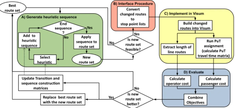
Fig. 4 Description of one iteration of the SSHH algorithm application in the global optimisation. Each
iteration begins with box A: The generation of the sequence of heuristics (see Sect. 5.1) and applying it to the current route set (see Sect. 5.3) to create a new route set. The new route set is tested for its feasibil-ity (see Sect. 5.4). If the new route set is not feasible, it is rejected and a new heuristic sequence is gener-ated. Otherwise, the new route set is converted to stop point lists (Box B, see Sect. 4.2). The stop point lists are implemented in Visum as line routes and an assignment is executed to extract the information necessary for the evaluation (Box C, see Sect. 5.5). The evaluation includes combining the objectives of passenger and operator costs (Box D, see Sect. 5.5.1). If according to the evaluation, the new route set improves the current best route set, it replaces the latter and the transition and sequence construction matrices are updated (see Sect. 5.1)
5.3 Low‑level heuristics
The hyper-heuristic algorithm manages a set of low-level heuristics to modify a given route set. All the low-level heuristics have been designed to follow the adja-cency relations defined by the adjaadja-cency matrix A when performing operations. If applying the operation on the selected routes and positions would create inva-lid connections, new routes and positions are selected instead. This increases the chance of generating feasible solutions.
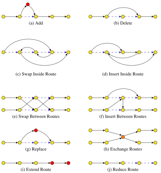
We give here a full list of the low-level heuristics applied in this work (also illustrated in Fig. 5):
– llh0 (Add): Selects a random route and a random position in this route. A new
vertex is selected and added in this position.
– llh1 (Delete): Selects a random route and random position and deletes the vertex in
this position.
– llh2 (Swap inside route): Selects a random route and two random positions. The two
vertices in these positions swap with each other.
– llh3 (Insert inside route): Selects a random route and two random positions. The
ver-tex in the first position is inserted in the second position.
– llh4 (Swap between routes): Selects two random routes and two random positions on
each of them. The vertices in these positions swap with each other.
– llh5 (Insert between routes): Selects two random routes and two random positions
on each of them. The vertex in the first position of the first route is inserted in the second position of the second route.
– llh6 (Replace): Selects a random route and a random position. The vertex in this
position is replaced by another selected vertex.
– llh7 (Exchange): Selects two random routes and splits them at a common vertex.
The parts of the two routes are exchanged to create two new routes. If the selected routes do not have a common vertex, a new pair of routes is selected.
– llh8 (Extend route): Selects a random route and adds vertices to the end of the route
until reaching another terminal.
– llh9 (Reduce route): Selects a random route and deletes vertices starting from the
last vertex in the route until reaching another terminal node.
5.4 Solution feasibility
Before implementing Snew into the Visum network model, a feasibility test is applied to
ensure that the route set satisfies all defined constraints in order to avoid wasting time in generating and evaluating many infeasible solutions. The feasibility constraints are defined with respect to the specifications in the Visum network model, for instance, backtracks and cycles are tolerated in the Visum network setup, while it is commonly considered a violation in most UTRP models. The full list of constraints is as follows: – The order of vertices on each route must follow the adjacency relations defined by
– Routes must start and end at the defined terminal vertices.
– Ring routes are allowed, but must start and end on the same vertex.
– The length of each route is within specified limits defined as input parameters by the user.
– No routes should fully overlap (this includes one route being sub-part of another). – Each zone must be connected to the route set: each zone in the Visum network
model must have at least one connector that is connected to an active stop point (i.e. a stop point used by at least one PuT line).
Fig. 5 Low-level heuristics set description. Straight arcs are edges in the route or added after applying
the heuristic, dashed arcs are edges removed after applying the heuristic, red nodes are nodes added after applying the heuristic
5.5 Evaluation
Depending on the objectives of the study and the available data, there are differ-ent ways to evaluate a route set. Transport modelling software packages like Visum come with a multitude of options to analyse the impact of changes in a transport net-work which can be used to construct a vast array of evaluation functions. Most nota-ble among Visum’s tools to model the impact of changes in a transport model are the assignment procedures used to calculate the flow of vehicles (PrT assignments) or PuT passengers (PuT assignments) through the network model. They provide out-put such as zone-to-zone travel time matrices (used in Sect. 5.5.1) or the load of vehicles on links (used in Sect. 5.5.2).
Assignment procedures, in general, start by determining all possible paths through the network model between all pairs of zones and their impedance. For PrT assignments, a specific PrT mode (e.g. private cars) has to be selected and the pos-sible paths calculated are constrained to the links which are open to this mode. PuT assignments determine the available paths on the network of all PuT lines. Possible interchanges between different PuT modes (e.g. between bus and train) are automati-cally taken into account.
The impedance of a path includes all time costs6 associated with the traveller. For
PrT, the impedance is defined by factors like the allowed speed on the links, turn penalties and time losses due to congestion effects. For PuT, the main factor of the path impedance is the perceived journey time, which is defined as weighted sum of several factors7, such as:
– Access time from origin zone to origin stop point (usually via the mode “walk-ing”).
– Waiting time at origin stop point. – Total in-vehicle travel time. – Penalty for the number of transfers.
– Walking time between stop points at transfers. – Waiting time at transfers.
– Access time from destination stop point to destination zone (usually via the mode “walking”).
Of particular importance are the transfer waiting times, which are the factors that distinguish between the two distinctive PuT assignment models used in this work: the headway-based and the timetable-based assignment. While the former assumes a fixed waiting time between vehicles for all routes, the latter derives the waiting times from a concrete timetable. Once all paths are determined, the assignment
6 Other costs, such as monetary costs, can be defined as well. However, these do not play a role in the present study.
7 Other factors, such as boarding time, can also be added, but it does not play a role in the present study. The weightings of the different factors can be set freely. In this study we used Visum default configura-tions where all time factors are weighted equally and the transfer penalty is set to 10 minutes per transfer.
distributes8 the trips given in the demand matrix over the available paths based on
their impedance. The resulting trips distribution allows us to estimate, for example, the number of vehicles that use a certain link (i.e. the link load).
The results of the assignments can be accessed in a number of different ways to generate evaluation functions. In the following, we introduce two evaluation meth-ods: the global optimisation and the local optimisation. The former uses a travel time matrix generated from the perceived journey time. The latter accesses the vehi-cle loads on selected links.
5.5.1 Global optimisation
Global optimisation is the method used by the vast majority of the UTRP studies: an objective function that aggregates information from the entirety of the system. We have chosen to use the sum of two relatively simple components for our objective function.
The first objective is to reduce the passenger cost (i.e. the average perceived jour-ney time of passengers). It is given by the following equation:
where Di,j is the PuT travel demand from a zone i to a zone j, and |Z| is the total
number of zones. 𝛩i,j is the shortest perceived journey time from zone i to zone j
using the PuT network defined by the solution S. The matrix 𝛩 can be generated
dur-ing the execution of the PuT assignment.
The second objective is the reduction of the operator costs. We have used a sim-ple approximation for the operators expenditures given by the total sum of travel times for travelling all the line routes in the PuT network:
where 𝜏i is the total travel time of line route i and |lr| is the total number of line
routes. The value of 𝜏i can be easily extracted from the network model using Visum
COM-API.
The two objectives are combined into a single objective function in the form of a weighted normalised sum given by the following formula:
(1)
CP(S) =
∑�Z�
i,j=1Di,j⋅𝛩i,j(S)
∑�Z� i,j=1Di,j (2) CO(S) = |lr| ∑ i=1 𝜏i(S) (3) fglobal(S) =𝛼 CP(S) CP(S0)+𝛽 CO(S) CO(S0)
8 The used distribution models are one of the main differences between the available assignment pro-cedures. More details of these procedures and their distribution models are explained in Visum manual (PTV AG 2018).
where S0 is the initial solution. The two weighting factors 𝛼 and 𝛽 can be adjusted
in relation to one another to generate solutions that are more favourable for either operators or passengers.
5.5.2 Local optimisation
For the local optimisation, we take advantage of two features in Visum. The first is that the assignment results can be easily accessed at a very localised level, e.g. the vehicle load of a particular transport mode on an individual link. The second is the ability to combine PuT and PrT assignments with a mode choice procedure. The mode choice procedure takes as input a demand matrix with all trips, and dis-tributes them into PuT trips and PrT trips. The distribution9 is based on the
imped-ance of the possible paths in the respective modes (PTV AG 2018). The results are separated into PuT and PrT demand matrices which are then used by the respective assignment procedures to assign the trips to travel paths. This combined procedure sequence allows us to analyse the effects of changes in the infrastructure on different transportation modes.
For the local objective function, we select a group of links L (e.g. links in a spe-cific neighbourhood), run the above-mentioned combined procedure sequence and sum up the load of private cars (i.e. PrT mode) on these links. The objective is to minimise the load of private cars on the selected links given by:
𝜈i(S) is the load of private cars on link i∈L while the travellers in the network can
choose between travelling via the public transport network defined by solution S, or by private cars. The link load is a standard output for most PrT assignments avail-able in Visum 17 (PTV AG 2018).
However, optimising a single objective can lead to very extreme solutions that are undesirable from other perspectives10. In order to avoid this we have used the global
objectives introduced in the previous section as bounding factors:
where S0 is the the initial solution and 𝜆P and 𝜆O are factors to determine how
much of an increase in the global objectives of solution S over their initial values is deemed acceptable to consider solution S.
(4) CL(S) = |L| ∑ i=1 𝜈i(S) (5) flocal(S) = { C L(S) CL(S0) if CP(S)≤𝜆P⋅CP(S0)and CO(S)≤𝜆O⋅CO(S0) ∞ otherwise
9 For the experiment in Sect. 6.3 a nested logit distribution function was used. However, other distribu-tion funcdistribu-tions are available in Visum, including a gravity model. More details on them can be found in the Visum manual (PTV AG 2018).
10 For an example see the results from the passenger perspective presented Sect. 6.1 where the operator costs increase by a factor of 8.
We have chosen a relatively simple measure to show the validity of the concept of local optimisation. However, it is straightforward to generalise this concept and apply it to other scenarios. For example, it is possible to estimate noise and air pol-lution with the HBEFA extension module in Visum11 and access the results on link
level similarly to the PrT load. This would extend our methods to design PuT net-works that improve the situation in heavily polluted areas.
6 Empirical results 6.1 Test on a small instance
6.1.1 Setup
For the first set of experiments, we used the transport model from the Visum quick start tutorial. This network model was built in 2006 as a Visum training exercise, and is loosely based on the small town of Pfullingen, Germany, with around 18 thou-sand inhabitants. The network model is relatively small, containing 652 nodes and 1782 links, 81 zones, 35 stops and stop points, and only five bus lines. We slightly modified this network model to be able to test various aspects of the interface proce-dure. It was, for example, necessary to create one stop with more then one stop point to test the use of the conversion table (see Sect. 4.2). A detailed description of these changes can be found in Appendix A.1.
The optimisation in these experiments is based on the global evaluation method (Sect. 5.5.1). To calculate the perceived journey time matrix 𝛩 , we used the
head-way-based PuT assignment procedure. A fixed frequency of 10 min is defined for all lines. This assignment model does not require the generation of vehicle journeys for each changed line route, which improves the run time.
The termination condition on these experiments is defined by the number of suc-cessful iterations. A sucsuc-cessful iteration consists of generating a new feasible solu-tion, implementing it in Visum and evaluating it. The number of successful itera-tions before the hyper-heuristic terminates is set to 20,000.
6.1.2 Results
In the first set of experiments we tested the two selection methods SR and SSHH in three distinctive scenarios: the passenger perspective, the operator perspective, and the balanced perspective. Each of these scenarios is defined by a different set of parameters in Eq. 3: for the operator perspective, effectively only the operator cost was considered as we set 𝛼=10−6 and 𝛽 =1−10−6 . The opposite in the passenger
perspective, where the focus is set on the passenger cost by setting 𝛼=1−10−6 and
11 Unfortunately, such a scenario could not be included in this study, as the HBEFA module was not included in our academic license.
𝛽 =10−6 . In the balanced perspective, we create a balance between the two
objec-tives by setting both parameters to 𝛼=𝛽 =0.5.
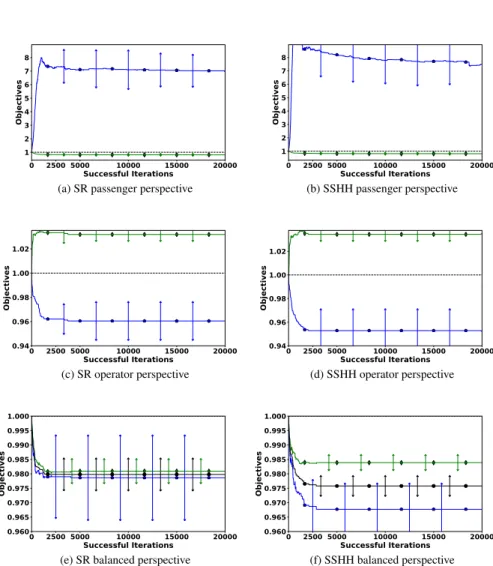
Figure 6 displays the change of the average passenger cost Cp(green line with
rec-tangles12), average operator cost C
O (blue line with pentagons (see Footnote 12)),
and the combined objective fglobal (black line with circles (see Footnote 12))
calcu-lated by Eq. 3. For each of the three scenarios the passenger and operator costs have been normalised using their initial values for better interpretation of their perfor-mance. The averages are calculated from the ten runs for each successful iteration.
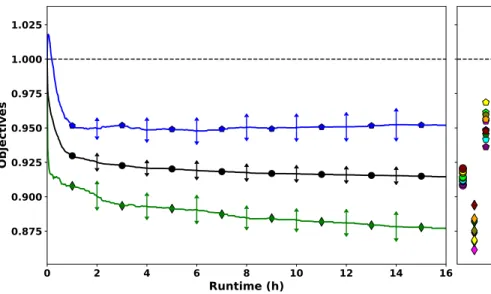
From the figures, it is clear that, from either the passenger or the operator per-spective, the objective that the optimisation is focusing on decreases rapidly from its initial value, while the other objective increases. This improvement starts to slow down at the 2000 iterations stage.
In the case of balancing the two objectives, both the passenger and operator costs show similar behaviour by dropping quickly at the beginning of the search and slow-ing down after 2000 iterations. The SSHH selection method was more successful in this case in improving the operator cost, while both selection methods reduced the passenger cost at a similar rate.
Table 1 summarises the results of the passenger and operator costs for the ten runs normalised and averaged. The best results and the standard deviation are also recorded. From this table, the most notable improvement is in the passenger perspec-tive with a reduction of 20% in the passenger cost from the initial values, although this was at the expense of significantly increasing the operator costs. The operator perspective runs reduced the operator cost on average by almost 7%, and the bal-anced runs recorded an improvement of nearly 5% on the operator cost, while the passenger cost is also improved by 3%.
The performance difference between the two selection hyper-heuristics is very small as can be seen from the table, but two observations were made during the experiments: the SSHH selection method was able to improve more in fewer itera-tions compared to simple selection, and this fact is critical for working with larger networks. Second, the SSHH recorded better individual results for the runs in many cases, especially from the operator perspective. Based on these facts we have selected the SSHH to be applied in the next set of experiments on a larger network model and to test the concept of local optimisation.
6.2 Application on city size network
6.2.1 Setup
In order to show the validity of the presented methods on a larger scale, another set of experiments has been performed on a network model originating from a real-world planning process. It was generated in the 1990s for the city of Halle, Germany,
12 The position of the markers (rectangle, pentagon and circle) have no meaning other than distinguish-ing the lines.
Fig. 6 Results of the global optimisation on a small network model for three scenarios: passenger per-spective, operator perper-spective, and balancing the two objectives using two selection hyper-heuristics (SR and SSHH). Each figure displays the development of the normalised passenger objective CP averaged for
ten runs (green with rectangles) the normalised averaged operator objective CO (blue with pentagons) and the averaged combined optimisation function fglobal (black with circles). The averages were calcu-lated for every successful iteration from ten independent runs. The bars in the middle represent the stand-ard deviation between the runs. Note: The position of the markers (rectangle, pentagon and circle) have no meaning other than distinguishing the lines
with over 200 thousand inhabitants. The model is made up of 1934 nodes, 4832 links, 81 zones, 288 stops and 313 stop points, and in total 41 PuT lines of which 18 are bus lines. Since 1996, this model has formed the basis of many Visum training examples, and therefore it is currently included in all Visum installations. Although this model has been modified over time, its size and layout are sufficient to represent a real-world network model. We only made very small modifications for the purpose of this work which can be found in Appendix A.2.
The Halle network model includes several modes of public transport: bus, tram and train. The optimisation is only applied on the bus lines, leaving the lines of the other modes unchanged. The frequency of the bus lines is set to 10 min. In these experiments, we used the timetable-based PuT assignment, which bases the inter-change waiting times on a timetable generated from departure and drive times. This way, the frequencies of the unchanged PuT lines are accurately reflected. However, the use of the timetable-based assignment requires adding vehicle journeys to the modified bus lines to define the bus timetable.
The termination condition for these experiments is set to run time rather than iterations, where each experiment is run for 16 h before it terminates. This was done for practical reasons and resulted in an average of 8919 successful iterations (i.e. on average 6.6 s per successful iteration13) for each run.
6.2.2 Results
Ten runs were applied on this transport network using the sequence-based selection with the balanced configuration. This configuration was chosen as an example of a planning process which requires a compromise between passengers and operators. Figure 7 shows the development of the average value of the passenger cost CP (green
with rectangles (see Footnote 12)), the operator cost CO [blue with pentagons (see
Footnote 12)], and the objective calculated by the combined optimisation function
Table 1 Results from passenger, operator, and balanced configurations for the two selection hyper-heuristics
The results are normalised and averaged over the ten runs. The standard deviation and the best results are also recorded
Scenario Obj SR-IE SSHH-IE
Avg Std Min Avg Std Min Passenger Cp 0.81 0.005 0.80 0.81 0.006 0.80 Co 6.96 1.07 5.12 7.49 1.55 6.46 Operator Cp 1.03 0.004 1.02 1.03 0.004 1.02 Co 0.96 0.014 0.93 0.96 0.014 0.93 Balanced Cp 0.98 0.003 0.97 0.96 0.008 0.96 Co 0.98 0.014 0.96 0.96 0.008 0.96
13 We used a desktop PC with an Intel i3-4150 3.50 GHz Dual Core CPU and 16 GB RAM for these experiments.
fglobal (Eq. 3) [black with circles (see Footnote 12)] over time. The error bars show
the standard deviation between the different runs.
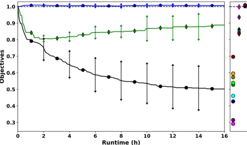
For this network, it can be observed that at the early stages of the search, the pas-senger objective steadily decreases, while the very early solutions show an increase in the operator cost. However, over the search time, the operator cost drops below its initial values but hovers around a value of 0.95, unlike the passenger cost which continues to drop until the end time of the search for most runs. After 16 h, the pas-senger cost reaches on average a value of 0.877.
The right side bar in Fig. 7 displays the final values of CP (rectangles), CO
(pen-tagons), and the combined objective fglobal (circles) for each of the ten runs. The
Fig. 7 Results for PuT line global optimisation with SSHH on a city sized network. Displayed is the
development of the normalised average passenger objective CP (green with rectangles), the operator
objective CO (blue with pentagons) and the combined optimisation function fglobal (black with circles). The averages were calculated in steps of one minute from ten independent runs. The bars show the stand-ard deviation between the runs. The markers at the right side bar show the distribution of the final values of the individual runs after 16 h of run time (also shown in Table 2). Each marker represents the final value of either fglobal (circles), CP (rectangles), or CO (pentagons) for each run. Each colour uniquely
identifies one of the ten experiments. Note: The position of the markers (rectangle, pentagon and circle) have no meaning other than distinguishing the lines
Table 2 Final values of ten runs with global SSHH optimisation
Values normalised on initial values and minimal values are highlighted in bold
1 2 3 4 5 6 7 8 9 10 Avg
fglobal 0.912 0.917 0.914 0.911 0.919 0.914 0.909 0.908 0.921 0.920 0.915
CP 0.882 0.875 0.868 0.874 0.868 0.882 0.882 0.862 0.894 0.884 0.877
objective values belonging to one run are given the same marker colours. These val-ues are also shown in Table 2. We see that while for the operator cost CO , the
reduc-tion is between 3.1 and 6.4%, for the passenger cost CP larger reductions between
10.6 and 13.8% are achieved.
Interestingly, the two runs with the highest reduction in CO and CP , respectively,
are also the two best runs in terms of combined reduction of both objectives. The run reducing CO by 6.4% reduced CP by 11.8%, and the run which reduced CP by
13.8%, also reduced CO by 4.5%. This shows that improvements in both objectives
are not mutually exclusive.
6.3 Application of local optimisation
6.3.1 Setup
For testing the local optimisation we used the transport model of the Visum 17 example “Demand NestedLogit” which comes with an implemented mode choice procedure for the mode choice between the PrT and PuT modes. The network model is identical to the one used in Sect. 6.2 and was subjected to the same modifications.
The predefined assignment procedures are split to separate assignments for the morning and evening peak traffic using different demand matrices. However, only the output from the morning peak (with the settings unchanged) is used in our study, to keep the application of our methodology as simple as possible. The applied assignment procedure for PuT is the timetable-based assignment, and vehicle jour-neys were set to start with an interval of 10 min.
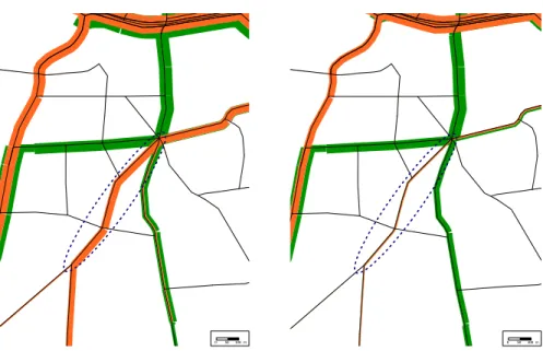
As stated in Sect. 5.5.2, the target of the local optimisation is to reduce the load of private cars on a selected number of links. For this purpose, we selected the links with the ID-numbers 178, 186, and 4048, which represent the street Wörm-litzer Straße in the city of Halle. This street is an important connector about 1 km south of the main city centre. As bounding factors, we have chosen 𝜆P=1.05 and
𝜆O=1.01.14 We again used the 16 h run time. However, due to the more complex
sequence of procedures required for the evaluation, the average length of a suc-cessful iteration during the experiments was 83.8 s, leading to an average number of successful iterations of 765.
6.3.2 Results
Ten independent runs were performed and the results are displayed in Fig. 8. The data lines show the time development of the average of the global passenger objec-tive CP (green with rectangles), and the operator objective CO (blue with pentagons),
respectively. The black line with circles shows the average of the local objective CL .
The bars show the standard deviation between the different runs.
14 The values of 𝜆P and 𝜆
O were chosen arbitrarily. They represent a maximal allowed increase of the

![Figure 7 shows the development of the average value of the passenger cost C P (green with rectangles (see Footnote 12)), the operator cost C O [blue with pentagons (see Footnote 12)], and the objective calculated by the combined optimisation function](https://thumb-us.123doks.com/thumbv2/123dok_us/896613.2615319/27.659.247.583.89.254/development-passenger-rectangles-footnote-pentagons-footnote-calculated-optimisation.webp)