Doctoral Dissertations Student Theses and Dissertations
Spring 2018
Adaptive dynamic programming with eligibility traces and
Adaptive dynamic programming with eligibility traces and
complexity reduction of high-dimensional systems
complexity reduction of high-dimensional systems
Seaar Jawad Kadhim Al-DabooniFollow this and additional works at: https://scholarsmine.mst.edu/doctoral_dissertations Part of the Computer Engineering Commons
Department: Electrical and Computer Engineering Department: Electrical and Computer Engineering
Recommended Citation Recommended Citation
Al-Dabooni, Seaar Jawad Kadhim, "Adaptive dynamic programming with eligibility traces and complexity reduction of high-dimensional systems" (2018). Doctoral Dissertations. 2657.
https://scholarsmine.mst.edu/doctoral_dissertations/2657
This thesis is brought to you by Scholars' Mine, a service of the Missouri S&T Library and Learning Resources. This work is protected by U. S. Copyright Law. Unauthorized use including reproduction for redistribution requires the permission of the copyright holder. For more information, please contact [email protected].
COMPLEXITY REDUCTION OF HIGH-DIMENSIONAL SYSTEMS by
SEAAR JAWAD KADHIM AL-DABOONI A DISSERTATION
Presented to the Graduate Faculty of the
MISSOURI UNIVERSITY OF SCIENCE AND TECHNOLOGY In Partial Fulfillment of the Requirements for the Degree
DOCTOR OF PHILOSOPHY in
COMPUTER ENGINEERING 2018
Approved by
Dr. Donald C. Wunsch, Advisor Dr. Jagannathan Sarangapani
Dr. R. Joe Stanley Dr. Maciej Zawodniok
SEAAR JAWAD KADHIM AL-DABOONI All Rights Reserved
PUBLICATION DISSERTATION OPTION
This dissertation has been prepared using the Publication Option. All papers are formatted in the style used by the Missouri University of Science and Technology, which are listed as follows:
Paper I: Pages 6 - 55; S. Al-Dabooni, and D. Wunsch, “Model Order Reduction Based on Agglomerative Hierarchical Clustering,” accepted inIEEE Trans. Neural Netw.
and Learn. Syst., 2017.
Paper II: Pages 56 - 87; S. Al-Dabooni, and D. Wunsch, “Heuristic dynamic pro-gramming for mobile robot path planning based on Dyna approach,” IEEE/INNS, Interna-tional Joint Conference on Neural Networks (IJCNN), pp. 3723 - 3730, Jul. 2016.
Paper III: Pages 88 - 113; S. Al-Dabooni, and D. Wunsch, “Mobile Robot Control Based on Hybrid Neuro-Fuzzy Value Gradient Reinforcement Learning,” IEEE/INNS, International Joint Conference on Neural Networks (IJCNN), pp. 2820-2827, May 2017.
The other papers are submitted to IEEE Trans. Neural Netw. and Learn. Syst.,
which are listed as follows: Paper IV: Pages 114 - 157; S. Al-Dabooni, and D. Wunsch, “The Boundedness Conditions for Model-Free HDP(λ).”
Paper V: Pages 158 - 208; S. Al-Dabooni, and D. Wunsch, “Online Model-Free N-Step HDP with Stability Analysis.”
Paper VI: Pages 209 - 261; S. Al-Dabooni, and D. Wunsch, “An Improved N-Step Value Gradient Learning Adaptive Dynamic Programming Algorithm for Online Learning, with Convergence Proof and Case Studies.”
Paper VII: Pages 262 - 325; S. Al-Dabooni, and D. Wunsch, “Convergence Analysis Proofs for Recurrent Neuro-Fuzzy Value-Gradient Learning with and without Actor.”
ABSTRACT
This dissertation investigates the application of a variety of computational intelli-gence techniques, particularly clustering and adaptive dynamic programming (ADP) designs especially heuristic dynamic programming (HDP) and dual heuristic programming (DHP). Moreover, a one-step temporal-difference (TD(0)) andn-step TD (TD(λ)) with their
gradi-ents are utilized as learning algorithms to train and online-adapt the families of ADP. The dissertation is organized into seven papers. The first paper demonstrates the robustness of model order reduction (MOR) for simulating complex dynamical systems. Agglom-erative hierarchical clustering based on performance evaluation is introduced for MOR. This method computes the reduced order denominator of the transfer function by clustering system poles in a hierarchical dendrogram. Several numerical examples of reducing tech-niques are taken from the literature to compare with our work. In the second paper, a HDP is combined with the Dyna algorithm for path planning. The third paper uses DHP with an eligibility trace parameter (λ) to track a reference trajectory under uncertainties for a non-holonomic mobile robot by using a first-order Sugeno fuzzy neural network structure for the critic and actor networks. In the fourth and fifth papers, a stability analysis for a model-free action-dependent HDP(λ) is demonstrated with batch- and online-implementation learning, respectively. The sixth work combines two different gradient prediction levels of critic networks. In this work, we provide a convergence proofs. The seventh paper develops a two-hybrid recurrent fuzzy neural network structures for both critic and actor networks. They use a novel n-step gradient temporal-difference (gradient of TD(λ)) of an advanced
ADP algorithm called value-gradient learning (VGL(λ)), and convergence proofs are given. Furthermore, the seventh paper is the first to combine the single network adaptive critic with VGL(λ).
ACKNOWLEDGMENTS
Thanks to my God for helping me and giving me the blessings to complete this work. I would like to thank my advisor, Dr. Donald C. Wunsch, for his continuous invaluable support me. Dr. Wunsch has given me the most professional guidance throughout choosing modern research topics, paper writing, technical presentations, and all required resources for producing good works.
I would like to express my sincere gratitude to all my committee members, Dr. Jagannathan Sarangapani, Dr. R. Joe Stanley, Dr. Maciej Zawodniok and Dr. Cihan Dagli, for their valuable advice and recommendations, and for their precious time in examining this dissertation. I am very grateful to the Higher Committee for Educational Development (HCED) in Iraq for granting me a Ph.D. scholarship and financial support. I am very thankful for my research group members in the Applied Computational Intelligence Laboratory (ACIL) for their fruitful discussion. They are wonderful praters and helpers.
Big thanks to my father, my mother, my brothers, and my sisters with all their nieces, nephews, and brothers-in-low for support, encouragement, and prayers throughout my study. I would also thanks Hassanin Al-Dabooni, Dr. Suadad Al-Dabooni, Dr. Alaa Al-Kinani, Seemaa Al-Dabooni, Dr. Hussein Shakarchi, and Dr. Turki Younis for their orientation and support.
Last but not least, I would like to thank to my friends Shahin Korkis Adam, Majid Hameed, Safaa Norri, Ahmed Adnan, Alaa Norri, Yassar Al-Tob, Wessam Al-Adbi, Yousif Khanjer, Mustafa Muzael, Ethar Alkamil, Ali Albattat, and Safaa Aiad for all the supports and encouragements.
TABLE OF CONTENTS
Page
PUBLICATION DISSERTATION OPTION . . . iii
ABSTRACT . . . iv
ACKNOWLEDGMENTS . . . v
LIST OF ILLUSTRATIONS . . . xiv
LIST OF TABLES . . . xxx
SECTION 1. INTRODUCTION. . . 1
1.1. SYSTEMS WITH REDUCING COMPLEXITY ... 1
1.2. ADVANCED ADAPTIVE DYNAMIC PROGRAMMING ... 1
1.3. RESEARCH CONTRIBUTIONS... 2
1.3.1. Model Order Reduction Based on Agglomerative Hierarchical Clus-tering... 2
1.3.2. Heuristic Dynamic Programming for Mobile Robot Path Planning Based on Dyna Approach... 3
1.3.3. Mobile Robot Control Based on Hybrid Neuro-Fuzzy Value Gradi-ent ReinforcemGradi-ent Learning ... 3
1.3.4. The Boundedness Conditions for Model-Free HDP(λ) ... 4
1.3.5. Online Model-Free N-Step HDP with Stability Analysis ... 4
1.3.6. An Improved N-Step Value Gradient Learning Adaptive Dynamic Programming Algorithm for Online Learning, with Convergence Proof and Case Studies ... 5
1.3.7. Convergence Analysis Proofs for Recurrent Neuro-Fuzzy
Value-Gradient Learning with and without Actor ... 5
PAPER I. MODEL ORDER REDUCTION BASED ON AGGLOMERATIVE HIERARCHI-CAL CLUSTERING. . . 6
ABSTRACT ... 6
1. INTRODUCTION ... 7
2. PROBLEM STATEMENT ... 11
3. HIERARCHICAL CLUSTERING SYSTEM POLES ALGORITHM ... 11
3.1. Choice of Distance Measure... 12
3.1.1 Hierarchical Cluster Poles Based on Euclidean-distance .. 12
3.1.2 Hierarchical Clustered Poles Based on MSE ... 13
3.2. Determining Transfer Function Coefficients ... 15
3.2.1 PA Method ... 15
3.2.2 GA Method... 17
4. SIMULATION AND ANALYSIS RESULTS WITH NUMERICAL EX-AMPLES ... 18
4.1. Comparative Studies From Published Literature ... 18
4.2. Case Study for Large Order System (Building Model Structure) ... 21
5. MODEL REDUCTION FOR A MULTIVARIABLE DYNAMIC MODEL BY USING HC-PE ... 26
6. CONCLUSION ... 41
APPENDICES . . . 47
A. Stability guarantee for a new reduced model . . . 47
C. Comparison table of HC-PE with other reduction methods, combining the Pade
approximation approach and GA. The best MSE results are shown in bold. . . 51
ACKNOWLEDGMENT ... 53
BIBLIOGRAPHY ... 53
II. HEURISTIC DYNAMIC PROGRAMMING FOR MOBILE ROBOT PATH PLAN-NING BASED ON DYNA APPROACH . . . 56
ABSTRACT ... 56
1. INTRODUCTION ... 57
2. COLLISION-FREE NAVIGATION ... 59
2.1. Simulation of Mobile Robot Platform... 59
2.2. Description of the Fuzzy Controller for Obstacle Avoidance ... 60
2.2.1 Distance ... 61
2.2.2 Angle ... 61
2.2.3 Angular Speed ... 61
3. FUNDAMENTAL REINFORCEMENT LEARNING PARAMETERS ... 64
4. MOBILE ROBOT PATH PLANNING BASED ON DYNA-HDP ... 66
4.1. Architecture of The Dyna-HDP System ... 66
4.2. k-max Certainty Method ... 69
4.3. Knowledge Sharing for Distributed Mobile Robots ... 70
5. SIMULATION RESULTS AND ANALYSIS ... 76
5.1. Applying Dyna-HDP in A New Environment (Building Map) ... 83
6. CONCLUSION ... 85
BIBLIOGRAPHY ... 85
III. MOBILE ROBOT CONTROL BASED ON HYBRID NEURO-FUZZY VALUE GRADIENT REINFORCEMENT LEARNING . . . 88
ABSTRACT ... 88
2. FUNDAMENTAL PRELIMINARIES... 90
2.1. Dynamic Modeling of the Mobile Robot ... 90
2.2. DP/RL Algorithms ... 93
2.3. FNN... 95
3. MOBILE ROBOT CONTROL BY FNN-BASED OF VGL(λ)... 96
3.1. VGL(λ) Structure Learning by Using FNN... 96
3.2. Mobile Robot Control Based on FNN-VGL(λ) ... 98
3.2.1 Critic Network Training Algorithm ... 99
3.2.2 Actor Network Training Algorithm ... 101
4. SIMULATION RESULTS ... 102
4.1. First Case (Effectiveness ofλvalue) ... 102
4.2. Second Case (with/without Actor Network) ... 103
5. CONCLUSION ... 111
BIBLIOGRAPHY ... 111
IV. THE BOUNDEDNESS CONDITIONS FOR MODEL-FREE HDP(λ) . . . 114
ABSTRACT ... 114
1. INTRODUCTION ... 115
2. STRUCTURE OF MODEL-FREE HDP(λ) ... 116
2.1. HDP(λ) Learning Views ... 116
2.2. The Critic Neural Network ... 121
2.3. The Actor Neural Network ... 123
3. STABILITY ANALYSIS ... 125
3.1. Lyapunov Approach... 125
3.2. Preliminaries ... 126
3.3. The Dynamical System Stability Analysis ... 129
4.1. Case I: Nonlinear System Problem ... 133
4.2. Case II: Inverted Pendulum ... 134
4.3. Case III: 3-D Maze Problem... 142
5. CONCLUSION ... 153
BIBLIOGRAPHY ... 154
V. ONLINE MODEL-FREE N-STEP HDP WITH STABILITY ANALYSIS. . . 158
ABSTRACT ... 158
1. INTRODUCTION ... 159
2. THE ONLINE MODEL-FREE NSHDP(λ) ... 162
2.1. NSHDP(λ) Architecture ... 162
2.2. The One-Step Critic Network (CN(0)) ... 166
2.3. The N-Step Critic Network (CN(λ)) ... 168
2.4. Actor Network (AN) ... 170
3. STABILITY ANALYSIS FOR NSHDP(λ) ... 172
3.1. Basics of The Lyapunov Approach ... 173
3.2. Assumptions... 174
3.3. The Stability Analyses for The Dynamical System... 178
4. SIMULATION STUDY ... 182
4.1. First Case: Nonlinear System Problem ... 183
4.2. Second Case: Inverted Pendulum ... 189
4.2.1 Description for The Inverted Pendulum Dynamic Model.. 189
4.2.2 Simulation Results ... 191
4.3. Third Case: 2-D Maze Problem ... 196
5. CONCLUSION ... 204
VI. AN IMPROVED N-STEP VALUE GRADIENT LEARNING ADAPTIVE DY-NAMIC PROGRAMMING ALGORITHM FOR ONLINE LEARNING, WITH
CONVERGENCE PROOF AND CASE STUDIES . . . 209
ABSTRACT ... 209
1. INTRODUCTION ... 210
2. THE ONLINE NSVGL(λ) STRUCTURE DESIGN ... 214
2.1. Improved Leaning of Temporal Sequences ... 214
2.2. Improved Exploration\Exploitation Trade-off ... 216
2.3. Memory Efficiency... 219
2.4. Improved Actor Network Training ... 220
2.5. Faster Convergence Via Two-Critic Iteration ... 221
3. CONVERGENCE PROOF ... 221
3.1. One-step andn-step DT-HJB Equations ... 221
3.2. Derivation of Iteration NSVGL(λ) Algorithm ... 224
3.3. Convergence of Iterative NSVGL(λ) Algorithm... 225
4. NEURAL NETWORK ARCHITECTURE DESIGN ... 234
4.1. The One-Step Critic Network Gˆ0 xk,ωˆc0 ... 234
4.2. Then-step Critic Network ( ˆGλ xk,ωˆcλ ) ... 236 4.3. Actor Network ( ˆA xk,ωˆa )) ... 237 5. SIMULATION STUDIES ... 239
5.1. Case I: Nonlinear System Problem ... 240
5.2. Case II: Mobile Robot Dynamic Model... 245
6. CONCLUSION ... 255
BIBLIOGRAPHY ... 256
VII. CONVERGENCE ANALYSIS PROOFS FOR RECURRENT NEURO-FUZZY VALUE-GRADIENT LEARNING WITH AND WITHOUT ACTOR. . . 262
1. INTRODUCTION ... 263
2. THE ACTOR-CRITIC AND SINGLE-CRITIC OF VGL(λ) ARCHITEC-TURE DESIGNS ... 266
2.1. Adaptive Actor-Critic Approach ... 269
2.1.1 The n-step Critic Network ... 269
2.1.2 The Actor Network ... 271
2.2. Single Adaptiven-step Critic Approach ... 272
2.2.1 The n-step Optimal Control Equation ... 272
2.2.2 The n-step Critic Network ... 272
3. NF STRUCTURES FOR VGL(λ) AND SNVGL(λ) APPROACHES... 274
3.1. Recurrent Neuro-Fuzzy (RNF) Structure ... 274
3.2. Takagi-Sugeno Recurrent Neuro-Fuzzy (TSRNF) Structure... 277
4. CONVERGENCE ANALYSIS OF THE VGL(λ) AND SNVGL(λ) AP-PROACHES ... 282
4.1. DT-HJB Equation for Rλ(k)... 282
4.2. Derivation of Iteration VGL(λ)... 285
4.3. Convergence of Iterative VGL(λ) Algorithm ... 286
5. COMPACTING THE NF-VGL(λ) AND NF-SNVGL(λ) ITERATIVE AL-GORITHM WITH RNF AND TSRNF STRUCTURES ... 292
5.1. The Value-Iteration-based NF-VGL(λ) ... 293
5.1.1 Then-step Critic Network ... 293
5.1.2 The Actor Network ... 294
5.2. The Value-Iteration-based NF-SNVGL(λ)... 295
5.2.1 Then-step Critic Network ... 295
5.2.2 Then-step Optimal Control ... 295
6. SIMULATION STUDY ... 296
6.1. The Nonlinear Dynamic Model of Mobile Robot ... 296
7. CONCLUSION ... 319 BIBLIOGRAPHY ... 319 SECTION
2. SUMMARY AND CONCLUSIONS . . . 326 2.1. MODEL ORDER REDUCTION BY CLUSTERING SYSTEM POLES ... 326 2.2. ADAPTIVE DYNAMIC PROGRAMMING WITH N-STEP PREDICTION
PARAMETER ... 327
BIBLIOGRAPHY . . . 329 VITA . . . 341
LIST OF ILLUSTRATIONS
Figure Page
PAPER I
1 General diagram for using HC-PE to reduce high order models. Any system model is built by deriving physical laws (physical modeling) or by observing data (identification modeling). Some models are represented by partial differ-ential equations (e.g. heat transfer equation), and other models are built by ordinary differential equations (e.g. robotics). Finite difference techniques are used to discretize partial differential equations to derive a numerical approx-imation for ordinary differential equations [3]. In this work, we focus on the models, which are built by using ordinary differential equations (G). In
combi-nation with PA or GA, HC-PE improves the evaluation for the reduced model (Gr) through selecting minimum MSEs of clusters made from poles. To find
the minimum MSE, all MSE values should be calculated for each level (order). MSE is calculated between the original model and the reduced models which is represented by the blue dashed line. ... 10 2 Three cases that should be considered while clustering poles using either
Euclidean-distance or MSE as the similarity. The first case is clustering real and complex poles separately. The second case is applying a full-state feed-back approach (pole placement method) in unstable systems. The third case is retaining the poles in the imaginary axis and in the origin of the s-plane to the reduced model. ... 14 3 Flowchart for the HC-PE algorithm, which starts fromnthorder and calculates
the reduced model inrth = nth−1 order, which becomes the base model (an
optimal simulated original model atrthorder) to calculate a next reduced model nth−1 order and so on until reaching the 2ndorder. ... 16
4 The dendrogram for hierarchical cluster poles based on Euclidean distance for
G10(s)combined with the PA approach. It clearly has large error values in most
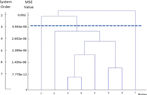
reduction orders. ... 20 5 The dendrogram for hierarchical clusters poles based on the HC-PE-PA
algo-rithm for G10(s). Minimum error and stability in the levels are generated by
using this algorithm. Cutting is done at level two to generate the 2nd order
reduced model for comparing [19] and [21]. ... 21 6 The Time Step response for step responses for original, [19] and [21], and
7 The dendrogram for hierarchical clustering of poles based on the HC-PE-PA algorithm for G8(s). Stability and fluent minimum error tracking level is
generated by using this algorithm. Level three was cut to generate a 3rd order
reduced model to compare with [19]. ... 23 8 The time step responses for the original, [19] and HC-PE-PA. ... 23 9 Bode plot for step responses for the original, [19] and HC-PE-PA to show the
stability. ... 24 10 Cluster poles of the Los Angeles building model. The blue star, red circle,
and green diamond shape symbols describe the best six clusters (three clusters in positive imaginary axis part with 3 mirror them in negative imaginary axis part), which is obtained by applying the HC-PE technique. The new system poles reduced model (six cluster centers) show as two big symbols (blue stars, red circles, and green diamonds). ... 27 11 A comparison between random (mode 1) and semi-random (mode 2) initial
chromosomes in population for 3 independent runs. Bold blue and red curves are a mean of mode 1 and mode 2, respectively, while thin blue and red curves are represented upper and lower fitness values for 3 runs. ... 28 12 The time step responses for the 48th order original building model and the
6th order reduced models obtained via HC-PE-PA, HC-PE-GA, Hankel and
balanced truncation techniques. HC-PE has the best performance compared with the other two approaches. MSE for HC-PE-PA, HC-PE-GA, Hankel and balanced truncation are 1.758e−09, 6.807e−10, 3.089e−07, and 2.827e−08,
respectively. ... 29 13 The Bode plot frequency responses for the 48th order original building model
and the 6thorder reduced models obtained via HC-PE-PA, HC-PE-GA, Hankel
and balanced truncation techniques. HC-PE-PA has the best approximation compared with the others, which is clear from the lowest frequency range until 0.5Hz... 30 14 Configuration model of triple link inverted pendulum. ... 35 15 The step response results after applying HC-PE-PA to reduce the model of the
triple link inverted pendulum to 3rdorder. (a) The cart displacement. (b) The
lower angle. (c) The middle angle. (d) The upper angle. The original 8thorder
model reduces after applying RCG and LQRCG. ... 37 16 The step response after applying HC-PE-PA and HC-PE-GA to reduce the model
of a triple link inverted pendulum to 3rdorder. (a) The cart displacement. (b)
The lower angle. (c) The middle angle. (d) The upper angle. The original 8rd
17 The step response after applying HC-PE-PA and HC-PE-GA to reduce the model of a triple link inverted pendulum to 3rdorder after changing mass parameters.
(a) The cart displacement. (b) The lower angle. (c) The middle angle. (d) The upper angle. The LQRCG method is applied to make the original 8th order
model stable. ... 39 18 Simulink model of LQRCG applied to the triple link inverted pendulum for
original 8th and 3rd order reduced model after applying HC-PE for both Pade
approximation and GA control by PID control with a disturbance input. ... 42 19 The responses after applying the disturbance signal on the cart displacement
state for comparison among LQRCG, HC-PE-PA, and HC-PE-GA reduced models.(a) The cart displacement.(b) The lower angle. ... 43 20 The responses after applying the disturbance signal on the first state (cart
dis-placement) to compare LQRCG, HC-PE-PA, and HC-PE-GA reduced models. (a) The middle angle state. (b) The upper angle state. GA performs slightly better for the transient response, but PA has acceptable transient and superior steady state performance. ... 44 21 2-D simulation for a triple linked inverted pendulum model. (a), (b) and (c)
show the simulation for the HC-PE-PA reduced model starting from the 0 position to the final desired cart positions which are 4, 6 and 10, respectively. ... 45 PAPER II
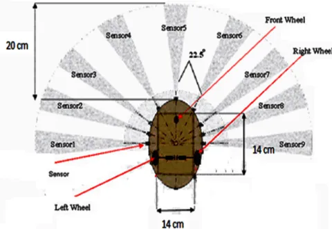
1 Differential wheeled mobile robot platform. It forms as 180◦ field of view in
front by nine sensors with 22.5◦separation angle to sense an object about 0.2
meter away from its body. ... 60 2 Distance fuzzy membership functions. These fuzzy set definitions are used for
input variable which are consisted from three triangular-shaped membership functions (good, near, and far). ... 61 3 Angle fuzzy membership functions. These fuzzy set definitions are used for
input variable which are consisted from five triangular-shaped membership functions (very negative, negative, zero, positive, and very positive). ... 62 4 Angular speed fuzzy membership functions. These fuzzy set definitions are
used for output variables for both left and right wheels which are consisted from five triangular-shaped membership functions (backward, slow backward, stop, slow forward, and forward). ... 62
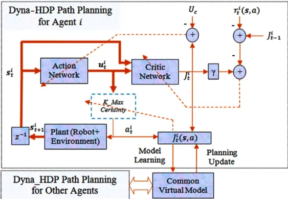
5 Block diagram for Dyna-HDP Path Planning. uit is the action vector at timet
for roboti which is consisted of three actions (turn left, turn right, and moving
forward) denoting asait. sit is the input states vector for robotiat timetwhich
are represented by the nine sensor readingsSd5−Sd9, the relative different angle
(θdi f f), and the relative distance (Dg). A reinforcement function (r) can get
from (2) for statesitandai. All robots share the same virtual model to maximize
the value functionJti for all agents at the same time. The backpropagation path
is shown by dashed lines for action and critic networks, and for updating the rules for k-max certainty. ... 66 6 A flow chart for k-max certainty selection procedure for agenti. A green dashed
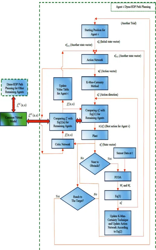
line border represents the exploitation approach which has been triggered by taking a greedy action among k-certainty rules (sensory-action pairs). The exploration approach is represented by a blue dashed line border which is selected action randomly among uncertainty rules (or trail). ... 71 7 Flowchart for implementation the multi-agents Dyna-HDP approach on maze
problem. ... 75 8 a) The environment for testing the exploration/exploitation strategy which shows
the initial start position for this agent. b) The near-optimality trajectory from the starting point to the target. c) The comparison betweenε−greedy and k-max
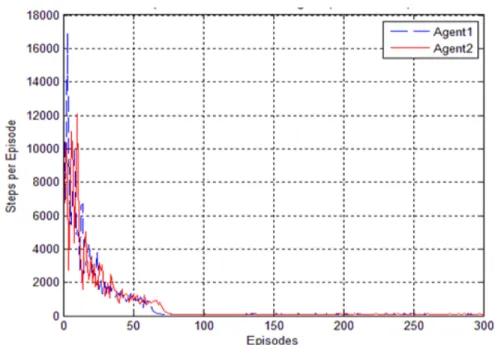
certainty by using Q-learning algorithm. ... 77 9 The first case comparison the number of steps per episodes. This compares
among Dyna-HDP with other conventional algorithms, one step Q-learning, Sarsa (λ), and Dyna-Q, for one agent (no information sharing with the others). . 79 10 The second case results (the cooperation between two agents by sharing their
ex-periences by using the Dyna-HDP approach). Every agent has own experience and tries to support the other one. ... 79 11 The Third case results (Cooperation among five agents by using the Dyna-HDP
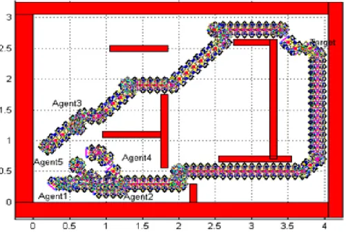
approach). ... 80 12 Five mobile robots are distributed in unknown environment surrounding by wall
in meter scale with many obstacles on it. The robots are distributed in random start position and heading angle to achieve same task (reaching to target position). 80 13 The near optimality trajectories for the five mobile robots from start positions
to the same target position after applying the third case which is all agents share their experiences with the same approach. ... 81 14 Comparison among all three cases by using Dyna-HDP for average learning.
In third case, the results are stable with the improvement in the learning speed of distributed autonomous agents by sharing their experiences. ... 82
15 a) The trajectories for two agents to run Task 1 b) The trajectories for two agents to run Task 2 c) The trajectories for one agent to run Task 3 d) The simulation result for three tasks among Dyna-HDP. ... 84 16 Path for mobile robot to implement the third task with a change in the
environ-ment by adding a new obstacle. FCOA gives the mobile robot the capability to adapt with this changing. ... 85 PAPER III
1 Schematic diagram of FNN used in ADP. Premise (σl i,m
l
i) and consequent
(cl1j, . . . ,c(ln+1)j) parameters are updated by using the backpropagation gradient
algorithm. The weights between the premise and hidden layers are always one. 97 2 Adaptation in VGL(λ) for the mobile robot trajectory control tracking. In
general, forward pathways are represented by the solid lines while pathways of backpropagation are shown by dashed lines, and the small solid black dots represent a connection. The sequential environment is used in this work by storing all states (velocity vectors) and actions (torque vectors) in forward pathways. The TD-error between ˜gt and ¯gt, as in (11), is used for updating
critic network weights with applying (23) for ¯gt. MUX box is used to feed
(23) as one thick dashed line by gathering the signals. The actor weights are updated by applying (24). For robustness testing, various values of ¯F and ¯τd
are injected into this dynamic model to examine the influences on τ(t). The
robot pose trajectory (xc,yc, θ) is obtained by using the mobile robot kinematic
equation (7) with fourth order Runge-Kutta integration for the derivative of the coordination and orientation of the robot. The Runge-Kutta integration also uses to solve the dynamic model (8) within 0.01 sec for the sample time. ... 100 3 The actor and critic performance atλ = 0. (a) Typical system trajectories for
both velocity states over time at last stable learning iteration. (b) The average of MSE for both velocity states over iterations. (c) The average torques applying to the left and right wheels over iterations. ... 104 4 The control performance atλ=0.9. (a) - (c) has same descriptions for (a) - (c)
as in Fig. 3. ... 105 5 Comparison of the average performance atλ = 0 and λ = 0.9. (a) The MSE
for both velocity state errors. (b) Requirement torque values. (c) The function value, which is calculated from (1). ... 106 6 Critic/actor and critic/optimal-torque approaches set to follow a circular
trajec-tory atλ=0.9 with disturbances for NN and FNN. (a) The X-Y trajectories for the mobile robot. ... 108
7 Critic/actor and critic/optimal-torque approaches set to follow a circular trajec-tory atλ= 0.9 with disturbances for NN and FNN. (b) and the average of MSE over iterations, respectively. (c) The absolute average values for the left and right control torques over iterations. ... 109 8 Critic/actor and critic/optimal-torque approaches set to follow a circular
trajec-tory atλ=0.9 with disturbances for NN and FNN. (d) The value of the torques over time for the last learning iteration for FNN. The cost-to-go value is shown in (e)... 110 PAPER IV
1 Schematic for the adaptation of the novel model-free HDP(λ) structure design according to (8). Forward pathways are represented by solid lines, while backpropagation pathways are shown by dashed lines. The small solid black dots represent a connection path. The initial target-values (¯v(t)) are provided
by substituting λ = 0 with (8), which is identical to the traditional HDP. The TD-error between ¯v(t − 1) and ˆv(t −1), as in (76), is used to update critic
network weights (84), which is represented by red dashed line. The actor network weights are estimated by back-propagating the prediction error (blue dashed line), which is equal to the value function (ˆv(t −1)) through the critic
network, and updating the actor’s weights according to (28)... 120 2 Schematic diagram of the critic network in HDP(λ). As mentioned by Werbos
in [30], this structure is more general than a traditional three-layer feedforward neural network by fully connecting all neurons. It models a variety of functional forms [34]. We set all weights that connect input nodes with output nodes to zero; therefore, it is similar to a three-layer feedforward neural network structure. ˆω{h}
c represents a hidden weights, which connect the input layer with
the hidden layer. The output weights are indicated as ˆω{o}
c , which connect both
input and hidden layers with the output layer. sk(t)is thekth hidden node input
of the critic network, and rk(t) is the corresponding output the hidden node.
Here, we only apply a hyperbolic tangent threshold function (φ(.)) to the hidden
neurons. ... 122 3 Schematic diagram of the actor network in HDP(λ). We set all weights that
connect input nodes with output nodes to zero as well as the connected weights between the outputs themselves. ˆω{h}
a represents hidden weights which connect
the input layer with the hidden layer. The output weights are indicated as ˆω{o}
a ,
which connect both input and hidden layers with the output layer. pk(t)is the kth hidden node input of the actor network, and qk(t) is the corresponding
output of the hidden node. Here, we only apply a hyperbolic tangent threshold function (φ(.)) on the hidden neurons. ... 124
4 Comparisons of system responses (the state vector trajectories and the action sequence) with HDP(λ=0.95), and traditional HDP(λ=0). ... 134
5 Cost error over iteration and 30 time step critic and actor errors. The upper figure shows the cost error over iterations, which clearly illustrates fast and stable learning, while traditional HDP shows fluctuations during learning. The critic and actor errors at the last learning iteration for HDP and HDP(λ) are shown in the middle and lower figures. ... 135 6 Learning weights for critic and actor networks for HDP and HDP(λ). ... 136 7 Configuration model of the cart-pole balancing system. ... 136 8 The value function and target value for the last trial without noise. The initial
angleθ(t)is 0.1◦... 138
9 Zoom-in between 80 to 220 time steps for Fig. (8). ... 138 10 Simulated results of balancing the inverted pendulum for control signal, θ(t),
andx(t)when the system is free of noise; initial angleθ(t)is 0.1◦. ... 139
11 Zoom-in between 400 to 520 time steps for Fig. (10). ... 139 12 The value function and target value for the last trial when the system is free of
noise; initial angleθ(t)is 10◦. ... 140
13 Zoom-in between 0 to 150 time steps for Fig. (12). ... 141 14 Simulated results of balancing the inverted pendulum for control signal, θ(t),
andx(t)when the system is free of noise; initial angleθ(t)is 10◦. ... 141
15 Zoom-in between 0 to 100 time steps for for Fig. 14. ... 142 16 Simulated results of balancing the inverted pendulum for control signal, θ(t),
andx(t)when the system has uniform 3% sensor noise; initial angleθ(t)is 10◦. 143
17 Simulated results of balancing the inverted pendulum for control signal, θ(t),
andx(t)when the system has uniform 3% sensor noise; initial angleθ(t)is 10◦. 143
18 The value function and target value for the last trial when the system has uniform 5% actuator noise; initial angleθ(t)is 10◦. ... 144
19 Simulated results of balancing the inverted pendulum for control signal, θ(t),
andx(t)when the system has uniform 5% actuator noise; initial angleθ(t)is 10◦.144
20 Squared critic error (Ec) for noise-free with 0.1◦to initial angle, noise-free with
21 Diagram of 3-D maze (5×5×5) with obstacles. The dark blue cube (0,0,0)
represents the initial position. The green cube (4,4,4) represents the target position. 12 obstacles are located in (0,3,0), (2,4,1), (2,4,2), (2,3,2), (2,2,2), (2,1,2), (4,0,0 − 4) and (3,0,4), which are represented by the red cubes.
Otherwise, the agent can move in free space. Three modes allow the agent to receive reward/cost values. First, The agent will receive reward 1 when it arrives to the target cube. Second, the agent will be punished by receiving -0.001 if it hits obstacles or passes the boundary. Third, the agent will receive 0 value as a reward in a free space. At any position in the maze, the agent has to select 1 action (direction) out of six actions in order to to move one step. The six actions are forward, right, backward, left, up and down, which can be seen in the figure as u1,u2,u3,u4,u5 and u6, respectively. We sketch this figure by
using the isometric drawing tool [42]. ... 150 22 Mean-squared-error (MSE) learning curves for SARSA(0), Q(λ=0.95), HDP(0)
and HDP(λ = 0.95) for the 3-D maze navigation benchmark as shown in Fig. 20. The mean values from 20 independent runs are taken for all methods. The shaded color represents the 20 runs, while the solid line represents the mean for all 20 runs. The HDP(0.95) approach has the fastest learning with a lower MSE compared to other approaches. ... 151 23 Summation of accumulative reward for every single episode of SARSA(0),
Q(λ= 0.95), HDP(0) and HDP(λ= 0.95) approaches, which is applied in the 3-D maze navigation benchmark as shown in Fig. 20. The mean values from 20 independent runs are taken for all methods. The shaded color represents the 20 runs, while the solid line represents the mean for all 20 runs. The HDP(0.95) approach reaches the largest accumulative reward compared to other methods. Because −greedy learning will reset the accumulative reward value every
episode, the accumulative reward values for Q(0.95), HDP(0) and HDP(0.95) converge over episodes. ... 152 24 −greedy learning curves for SARSA(0), Q(λ= 0.95), HDP(0) and HDP(λ=
0.95) approaches for 3-D maze navigation benchmark as shown in Fig. 20. These curves represent the number of steps per episode, where the agent returns back to the start cube only when it reaches the target cube. The mean values from 20 independent runs are taken for all methods. The shaded color represents the 20 runs, while the solid line represents the mean for all 20 runs. HDP(0.95) and HDP(0) have an almost identical number of steps over episodes, which are less than those in both Q(0.95) and SARSA(0) methods. ... 153
PAPER V
1 Schematic diagram for the adaptation of an online model-freen-step ADHDP
(NSHDP(λ)). This design uses two critic networks: the one-step critic network (CN(0)) and then-step critic network (CN(λ)). The CN(0) produces a
one-step-return value function (ˆv0(t)) based on the ordinary temporal-difference (TD)
learning algorithm, while the CN(λ) produces the average of then-step-return
value function (ˆvλ(t)) based on a TD(λ) learning algorithm [27]. The TD(λ)
learned from the average of then-step-return backups, whereλrepresents the
proportional average weight. λ−return (Rtλ) [16] is another name for the average
of the n-serp-return. The ˆvλ(t) value is identical to Rtλ, [29]. This design is
equivalent to the one-step TD backup (λ=0). It focuses on the recent information to predict the value function via CN(0). Online learning is another advantage of this design, where it speeds up the tuning without requiring any initial backup for ˆvλ(t). Furthermore, this design is a model-free learning design that does
not require prior knowledge about a mathematics dynamic model. Despite the bootstrapping eligibility trace parameters (λ and γ) give the CN(λ) the ability to determine a depth (effecting via λ) and a width (effecting via γ) from information during a sequence of events (i.e., the rewards in the backward view of TD(λ), [21]). The CN(0) provides the value function that concentrates on recent events. Therefore, the NSHDP(λ) design combines the details of the current information (real-time data) with a sequence of predicted events. This combination provides the optimal decisions [40] in the control/industry field as well as [41] in the consumer/marketing field (correlation between real time and history). The weights for CN(0) and CN(λ) are updated according to the TD(0) error (blue dashed line) and the TD(λ) error (green dashed line), respectively. The actor network (AN) that provides the action values is tuned by two paths (backpropagating errors): one through the CN(0) path (e0a(t)) and
the other through the CN(λ) path (eλa(t)). This strategy assists AN training to
correlate and combine the fluid information from CN(λ) and CN(0). These two paths are filtered via a similar value ofλ, and they combine to produce a total backpropagating actor error (red dashed line). ... 161 2 A schematic diagram of CN(0) in NSHDP(λ). As mentioned by Werbos in
[38], this structure is more general than a traditional three-layer feed-forward neural network that is fully connected among all neurons. It models a variety of functional forms as demonstrated in [39]. All weights were set so that the connection input nodes with the output nodes were zero. ˆω0{h}
c represents
hidden weights, which are connected to the input layer with the hidden layer. The output weights are indicated as ˆω0{o}
c , which connect both the input and
hidden layers with the output layer. ak(t) is the kth hidden node input of the
critic network, and bk(t) is the corresponding output of the hidden node. A
3 A schematic diagram of the averagen-step learning critic network (CN(λ)) in
NSHDP(λ). The ˆωcλ{h}represents the hidden weights which are connected to the
input layer through the hidden layer. The output weights are indicated as ˆωλ{o}
c ,
which connect both the input and hidden layers with the output layer. ck(t)is
thekth hidden node input of the critic network, anddk(t)is the corresponding
output to the hidden node. Here, only apply a hyperbolic tangent threshold function (φ(.)) is applied to the hidden neurons. ... 168
4 A schematic diagram of the actor network (AN) in NSHDP(λ). All of the weights that connect input nodes with output nodes are set to zero, as well as the connected weights between the outputs themselves. ˆω{h}
a represents the
hidden weights which are connected the input layer with the hidden layer. The output weights are indicated as ˆω{o}
a , which connect both input and hidden layers
with the output layer. pk(t)is the kth hidden node input of the critic network,
andqk(t)is the corresponding output to the hidden node. A hyperbolic tangent
threshold function (φ(.)) is applied in the hidden neurons. ... 171
5 Mean squared error comparisons over iterations among the NSHDP(λ), the GrHDP and the traditional ADHDP. NSHDP(λ) has a faster learning speed than the GrHDP and the ADHDP. ... 184 6 Comparisons of system response trajectories, which are the two system states
and the actions for the NSHDP(λ), GrHDP and ADHDP. ... 185 7 Comparisons for the value functions with their targets between the NSHDP(λ)
and the GrHDP. The upper figure shows the value function and its target for the GrHDP (see [7]), which is represented by a red dashed line in the upper figure part of Fig. 8. The middle and upper figures show the value functions of CN(0) and CN(λ) of the NSHDP(λ) with their targets (the left sides of Equations (10) and (11)), respectively. The solid green line in the lower part of Fig. 8 represents the difference of the middle figure, while the dashed red line represents the difference of the lower figure. ... 186 8 The squared critic errors. The upper figure shows the squared errors for critic
and reference networks in the GrHDP structure (see [7] Equations(4) and (5)). The squared critic errors for NSHDP(λ) for both critic networks (CN(0) and CN(λ)) are illustrated in the middle and upper figures when λ = 0.95 and λ=0, respectively. The squared error for the reference network in the GrHDP is represented by “Er”. ... 187 9 The upper figure shows the squared backpropagating actor error after passing
a critic network in the GrHDP. The middle and lower figures showBEa0(t)and BEaλ(t) (see (29)) of the NSHDP(λ) when λ = 0.95 and λ = 0, respectively.
The lower figure (NSHDP(0.95)) converges faster than the upper (GrHDP) and middle (ADHDP) figures ... 188
10 Learning weights for the NSHDP(λ) and the GrHDP. The upper, middle and lower figures in the first column show the learning weights during the time steps for CN(0), CN(λ) and AN in the NSHDP(λ), respectively. The upper, middle and lower figures of the second column show the learning weights during the time steps for goal representation or the reference network (RN), critic network and actor network of GrHDP... 189 11 The configuration schematic diagram of the inverted pendulum balancing system.190 12 Simulated results of balancing the inverted pendulum for u(t), θ(t), and x(t)
when the system is free of noise. The initial angleθ(t)is 0.1◦. ... 192
13 Zoom-in between 1000 to 1250 time steps for Fig. 12. ... 192 14 The value functions and their targets without noise. The backpropagating actor
errors are Be0a and Beλa through CN(0) and CN(λ), respectively. The initial
angleθ(t)is 0.1◦... 193
15 Zoom-in between 1000 to 1250 time steps for Fig. 14. ... 193 16 Simulated results of balancing the inverted pendulum to show u(t), θ(t) and
x(t), when the system is injected with 3% uniform noise to the actuator and
sensor. The initial angleθ(t)is−12◦. ... 194
17 The value functions and their target values with similar disturbances are in the caption of Fig. 16 (upper and lower figures for CN(0) and CN(λ), respectively). The backpropagation actor errors through CN(0) (Be0a) and CN(λ) (Beλa) are
shown in the lower figure. The initial angleθ(t)is−12◦. ... 195
18 Simulated results of balancing the inverted pendulum to show u(t), θ(t) and
x(t), when the system is injected with 3% uniform noise to the actuator and
sensor. The initial angleθ(t)is−12◦. ... 195
19 The function values with errors with the initial angleθ(t)is 12◦. The actuator
and sensor disturbances are similar to what in the caption of Fig. 18 ... 196 20 Diagram of a 2-D maze (7× 7) with obstacles. The point(0,0) represents the
initial position. The point (6,6) represents the target position. Eleven obstacles are located at (5,0), (6,0), (2,1), (5,2), (6,2), (2,3), (3,3), (6,3), (3,6), (0,6) and (3,6), which are represented as red squares. Otherwise, the agent can move in the free space. There are three modes where that the agent can receive reward/cost values. First, the agent will a receive reward of 1 when it arrives at the target. Second, the agent will be punished by receiving -0.001 if hits obstacles or passes the bound. Third, the agent will receive a 0 value as a reward in a free space. At any position in the maze, the agent has to select 1 action (direction) out of 4 actions in order to move one step. The 4 actions are forward, right, backward and left, which can be seen in the figure asu1,u2,u3
21 MSE Learning curves for the SARSA(0), Q(λ=0.95), ADHDP and NSHDP(λ= 0.95) methods for a 2-D maze navigation benchmark as shown in Fig. 20. The mean values from 20 independent runs are taken for all methods. The shaded color represents the 20 runs, while the solid line represents the mean for all 20 runs. The NSHDP(0.95) method learns the fastest and has the MSE compared to other methods. ... 202 22 A summation of the accumulative reward for every single episode for the
SARSA(0), Q(λ=0.95), ADHDP and NSHDP(λ =0.95) methods, which are applied in a 2-D maze navigation benchmark as shown in Fig. 20. The mean values from 20 independent runs are taken for all methods. The shaded color represents the 20 runs, while the solid line represents the mean for all 20 runs. The NSHDP(0.95) method has the largest accumulative reward compared to the other methods in the exploration moving mode. Because the−greedy
de-ceasing rate learning will reset the accumulative reward value at every episode, the accumulative reward values for the Q(0.95), ADHDP and NSHDP(0.95) are convergence over episodes. ... 203 23 −greedy learning curves for the SARSA(0), Q(λ = 0.95), ADHDP and
NSHDP(λ=0.95) methods for a 2-D maze navigation benchmark as shown in Fig. 20. These curves represent the number of steps per episode, where the agent returns to the starting point only when it reaches the target cube. The mean values from 20 independent runs are taken for all methods. The shaded color represents the 20 runs, while the solid line represents the mean for all 20 runs. The NSHDP(0.95) and the ADHDP have a nearly similar number of steps over episodes, which are less than both the Q(0.95) and the SARSA(0). ... 203 PAPER VI
1 Schematic diagram for the adaptation of a novel onlinen-step value gradient
learning (NSVGL(λ)). Two critic networks and one actor network are used in NSVGL(λ). A combination of two critic networks is presented to speed up the tuning for online learning without needing the initial backup value function and eligibility trace parameters. The weights for the one-step critic network ( ˆG0 xk,ωˆ0c
) and the
n-step critic network ( ˆGλ xk,ωˆλc
) are updated according to gradient of TD(0) error (blue dashed line) and gradient of TD(λ) error (green dashed line), respectively. The actor network ( ˆA xk,ωˆa
) is tuned by two paths (backpropagating errors): one through ˆG0 xk,ωˆ0c
path (
e0a) and the other
through ˆGλ xk,ωˆλc
path (eλa). This strategy can correlate and combine the
information from the two critic networks. These two paths are filtered via the same values ofλ, and they are added together to produce a total backpropagating actor error (red dashed line). ... 213 2 General feed-forward neural network, which is used in the one-step critic
3 The mean-squared-error (MSE) comparisons over iteration among NSVGL(λ= 0.99), NSVGL(λ = 0.5) and the DHP approaches. The mean values from 10 independent runs are taken for all methods. The shaded region represents 10 runs, while the solid line represents the mean for all 10 runs. NSVGL(λ) provides a faster learning speed than DHP. ... 241 4 The control input during iteration for NSVGL(λ=0.99), NSVGL(λ=0.5) and
the DHP. The mean values from 10 independent runs are taken for all methods. The shaded region represents the 10 runs, while the solid line represents the mean for all 10 runs. ... 242 5 The state trajectories for the x1 state during iteration for NSVGL(λ = 0.99),
NSVGL(λ=0.5) and the DHP. The mean values from 10 independent runs are taken for all methods. The shaded region represents the 10 runs, while the solid line represents the mean for all 10 runs. NSVGL(λ) improves faster than DHP. . 242 6 The state trajectories for the x2 state during iteration for NSVGL(λ = 0.99),
NSVGL(λ=0.5) and the DHP. The mean values from 10 independent runs are taken for all methods. The shaded region represents the 10 runs, while the solid line represents the mean for all 10 runs. NSVGL(λ) improves faster than DHP. . 243 7 The average gradient trajectories of the value functions for the first system state
in NSVGL(λ=0.99. The gradient of the cost functions gi0(x1k)andgiλ(x1k)
converge to the optimal value function. ... 244 8 The average gradient of the second cost function trajectories for the both critic
networks in the NSVGL(λ=0.99) approaches. The convergence of the gradient of the value functions for the second system state gi0(x2k)andgiλ(x2k)
to the optimal cost function is clearly shown starting from iteration number 200. ... 244 9 The average mean-squared-error for two velocity states during iterations among
NSVGL(λ = 0.99), NSVGL(λ = 0.5) and the DHP. The mean values from 10 independent runs are taken for all methods. The shaded region represents the 10 runs, while the solid line represents the mean for all 10 runs. NSVGL(λ) illustrates faster learning than DHP. ... 248 10 The first control input (left torque) during iterations among NSVGL(λ=0.99),
NSVGL(λ = 0.5), and the DHP. The mean values from 10 independent runs are taken for all methods. The shaded region represents the 10 runs, while the solid line represents the mean for all 10 runs. ... 249 11 The second control input (right torque) during iterations among NSVGL(λ =
0.99), NSVGL(λ= 0.5), and the DHP. The mean values from 10 independent runs are taken for all methods. The shaded region represents the 10 runs, while the solid line represents the mean for all 10 runs. ... 250
12 Comparisons of state trajectory for the first state (linear velocity) during iter-ations for NSVGL(λ = 0.99), NSVGL(λ = 0.5), and DHP approaches. The mean values from 10 independent runs are taken for all methods. The shaded region represents the 10 runs, while the solid line represents the mean for all 10 runs. NSVGL(λ) has better performance than DHP, whereas it is faster improved during iteration. ... 251 13 Comparisons of the state trajectories for the second state (angular velocity) for
NSVGL(λ = 0.99), NSVGL(λ = 0.5), and DHP. The mean values from 10 independent runs are taken for all methods. The shaded region represents the 10 runs, while the solid line represents the mean for all 10 runs. NSVGL(λ) learns faster than DHP. ... 252 14 The average gradient of the first state of value function trajectories for both
critic networks in the NSVGL(λ = 0.99). The gradient of the value functions
(gi0(x1k)andgiλ(x1k)) are converged to the optimal cost function. ... 253
15 The average gradient of the second state of the value function trajectories for both critic networks for NSVGL(λ= 0.99). ... 253
PAPER VII
1 A schematic diagram for the adaptation of actor-critic VGL(λ). The weights for the critic network ( ˆG x(k),ωˆc) are updated according to the gradient of the
TD(λ) error (black dashed line). The actor network ( ˆA x(k),ωˆa
) is tuned by backpropagating the actor error (ea) through ˆG x(k),ωˆc
network (red dashed line). ... 270 2 A schematic diagram for the adaptation of a single n-step critic network of
VGL(λ)(SNVGL(λ)). The weights for the critic network ( ˆG x(k),ωˆc) are
updated according to the gradient of the TD(λ) error (black dashed line). The general n-step optimal control equation (14) (or (73) for Affine systems with
the quadratic form of a utility function) is used to generate an optimal control signal. ... 273 3 A structure for RNF that uses both actor and critic networks for VGL(λ) and
NSVGL(λ). RNF consists of three layers. The first layer is the premise layer, which has premise parameters (mn×m,σn×m,θn×m). The second layer is the
rule layer, which hasmn rule nodes. The third layer is the consequent/output
layer, which has consequent parameters (ωp×mn). The premise and consequent parameters are trained by using a backpropagation gradient algorithm. To simplify the appearance of this diagram, the number of inputs, MFs and outputs are represented byn =3,m =2 and p=2, respectively. ... 278
4 A structure for TSRNF that uses VGL(λ) and NSVGL(λ). TSRNF consists of five layers. The first layer represents the premise layer, which has premise parameters (mn×m,σn×m,θn×m). The second layer is the rule layer, which has mnrule nodes. The third layer is the normalization layer to normalize the output
values coming from the rule layer. The fourth layer is the consequent layer, which has consequent parameters (amp×(n n+1)). The fifth layer is the output layer
to obtain the final output signal. The premise and consequent parameters are trained by using a backpropagation gradient algorithm. The number of inputs, MFs and outputs are represented byn =3, m=2 and p=2, respectively. ... 283
5 Average of MSEs for the two states for comparisons RNF-VGL(λ= 0) and RNF-VGL(λ=0.98) with an impact on disturbances and frictions. Five independent runs are taken. The shaded region represents the runs, while the solid line represents the mean of runs. RNF-VGL(λ = 0.98) allows for faster learning than RNF-VGL(λ= 0). ... 301 6 Initial and final learned Gaussian membership functions (GMFs) for both input
states (linear and angular velocities) to the critic network in RNF-VGL(0). ... 301 7 Initial and final learned GMFs for both linear and angular velocity input states
to the actor network in RNF-VGL(0). ... 302 8 Deviation of the recurrent parameters (θ) for both input velocity states from the
initialized values of the critic network of RNF-VGL(0) during all of the total training steps, which is 12000 iteration with 100 time steps each. ... 303 9 Deviation of the recurrent parameters (θ) for both input velocity states from the
initialized values of the actor network of RNF-VGL(0) during the total training steps. ... 304 10 Initial and final learned GMFs for both linear and angular velocity input states
to the actor network in RNF-VGL(λ). ... 305 11 Initial and final learned GMFs for both input states to the actor network in
RNF-VGL(λ). ... 305 12 Deviation ofθ for both input velocity states from the initialized values of the
critic network of RNF-VGL(λ) during all the total training steps. ... 306 13 Deviation ofθ for both input velocity states from the initialized values of the
actor network of RNF-VGL(λ) during the total training steps. ... 307 14 Average of MSEs for the two states for comparisons: RNF-VGL(λ) and
RNF-SNVGL(λ) with % = 0.001. Five independent runs are taken. The shaded region represents the runs, while the solid line represents the mean of the runs. RNF-SNVGL(λ) learns faster a faster learning than RNF-VGL(λ). ... 309
15 The X-Y circle trajectories for RNF-VGL(λ) and RNF-SNVGL(λ) with % = 0.001. The mean of five independent runs is shown. RNF-SNVGL(λ) is faster, but RNF-VGL(λ) performs better and improves with long training iterations. .. 310 16 The average of the right and left input torques for the dynamic mobile robot
for RNF-VGL(λ) and RNF-SNVGL(λ) with % = 0.001. The shaded region represents the runs, while the solid line represents the mean of the runs. ... 311 17 The average gradient of the two input velocity states of the value function
trajectories for the critic network in both RNF-VGL(λ) and RNF-SNVGL(λ). ... 312 18 The average of the MSEs for comparing the two states of TSRNF-VGL(λ) and
TSRNF-SNVGL(λ) with % = 0.001. Five independent runs are taken. The shaded region represents the runs, while the solid line represents the mean of the runs. TSRNF-SNVGL(λ) learns faster than TSRNF-VGL(λ). ... 314 19 The X-Y circle trajectories for TSRNF-VGL(λ) and TSRNF-SNVGL(λ) with
% = 0.001. The mean of five independent runs is shown. TSRNF-SNVGL(λ) learns faster, but TSRNF-VGL(λ) perfoms better ad improves with long training iterations. ... 315 20 The average of the right and left input torques to the dynamic mobile robot for
TSRNF-VGL(λ) and TSRNF-SNVGL(λ) with % = 0.001. The shaded region represents the runs, while the solid line represents the mean of the runs. ... 316 21 The average gradient of the two input velocity states of the value function
LIST OF TABLES
Table Page
PAPER I
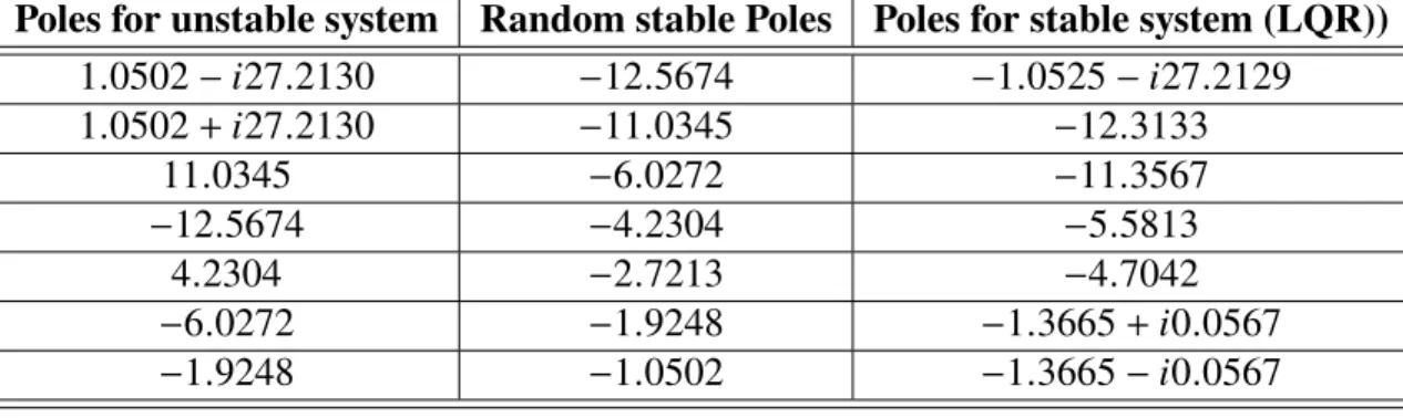
1 GA operations selection approach... 18 2 Poles values for unstable and stable for triple link inverted pendulum model... 33 3 List of abbreviations and symbols... 46 PAPER II
1 Right side controller rules matrix ... 63 2 Left side controller rules matrix ... 63 PAPER III
1 Parameters of the dynamic mobile robot... 103 PAPER IV
1 Performance evaluation of HDP(λ) learning controller when balancing the inverted pendulum dynamic system. The second and third columns depict the average number of trials it took to learn to balance the pole for 1000 time steps for HDP and HDP(λ) approaches, respectively. The average is based on 100 successful runs at 1000 iterations each. ∗ actuators are subjected to noise; #
sensors are subjected to noise ... 146 PAPER V
1 Performance evaluation of the NSHDP(λ) learning controller when balancing the inverted pendulum dynamic system. The third and fourth columns depict the average number of trials it took to learn to balance the pole for 100 time steps for the GRHDP and the NSHDP(λ), respectively. The average is taken over 100 successful runs for 5 iterations each. ∗actuators are subjected to noise;
#sensors are subjected to noise... 197
PAPER VI
PAPER VII
1 The values forα`
i. α
`
i depend oni and`. The rows for the last column (i = n)
increase by one with each`and replicate eachm. The rows for the column with i= n−1 increase by one each with each` = mand republicate eachm2and so
on... 275 2 Parameters of the dynamic mobile robot.
%is various random values to test the dynamic model performance in different frictions ... 299 3 MSE values for RNF-VGL(λ) and RNF-SNVGL(λ) with and withoutθrecurrent
parameters at various noise levels (different %values). All-iteration (All Iter) is the average of 12000 MSE, while final-iteration (Final Iter) is the MSE at the last iteration (12000th). ... 313 4 MSE values for TSRNF-VGL(λ) and TSRNF-SNVGL(λ) with and without θ
recurrent parameters at various noise levels (different %values). All-iteration (All Iter) is the average of 12000 MSE, while final-iteration (Final Iter) is the MSE at the last iteration (12000th). ... 318
1. INTRODUCTION
1.1. SYSTEMS WITH REDUCING COMPLEXITY
Because there are numerous physical systems have high order mathematical models in real world, these systems require a massive of a computational complexity to address, solve and simulate. Many algorithms are used to make these systems less complicated, while retaining the properties of the original system. These algorithms have a capability of simulating affordable prototypes with fast and reliable responses. Model order reduction (MOR) is applied in many fields, such as computational biology, mechanics, fluid dynamics, circuit design, and control systems. In this dissertation, the reduction focuses on control area, which analyzes the characteristics and features of dynamic systems to reduce their complexity while keeping their properties as possible as illustrated in the first paper in the paper section of this dissertation.
1.2. ADVANCED ADAPTIVE DYNAMIC PROGRAMMING
Adaptive dynamic programming (ADP) is a powerful tool that allows an agent to learn by interacting with its environment to obtain an optimal control policy. The ADP technique uses a heuristic method to overcome a nonlinearity behavior system that generates a difficulty to solve the Hamilton-Jacobi-Bellman equation instead of the Riccati equation. The ADP technique allows agents to select an optimal action to minimize their long-term cost value by solving the Bellman equation. A heuristic dynamic programming, a dual heuristic programming and a globalized dual heuristic programming are three fundamental categorizes for ADP technique. These categorizes consist of three approximation function
networks, which are actor, critic and model networks that provide decision making, eval-uation, and prediction, respectively. Because a model network, which predicts the future system state, is included within these categorize, the ADP categorizes as a model-based ADP design. If the action-dependent (AD) expression is used in the ADP, then the critic network has the state and the action inputs. A model-free ADP design has been presented for online learning, which is not required the model network. Many applications have used the ADP techniques. A temporal-difference (TD) with eligibility trace parameter is a more advanced learning algorithm than the traditional TD that combines basic TD learning with an eligibility traces technique to further accelerate learning. The ADP technique is used to train an actor network to give optimal actions based on minimizing a value function that is produced from a critic network. In this dissertation, all networks are approximated by using a multilayer perceptron neural network, and hybrid neuro-fuzzy networks. We investigate in ADP with advanced TD learning and new novel structures that make system more robust, fast and stable during training as presented in the second paper until seventh paper in paper section of this dissertation.
1.3. RESEARCH CONTRIBUTIONS
This dissertation deals with the use of reducing complexity of models and applying feature forward and backward views of eligibility trace procedures with ADP in various benchmarks tasks. In concrete, we describe each paper’s contribution as follows:
1.3.1. Model Order Reduction Based on Agglomerative Hierarchical Cluster-ing. The main contribution in this work is provided a model order Reduction (MOR)
technique that gives any required order of reduced model with a minimum MSE value. Instead of neglecting some poles like traditional methods, our approach engages all prop-erties of the original system by using agglomerative hierarchical clustering of system poles depending on a performance evaluation. Therefore, the method will be called HC-PE. HC-PE is effective for converting original high order ordinary differential equations to low
order equations. HC-PE with PA or GA takes the output response(s), and it calculates the MSE between the original model and the reduced model. It uses an improved modified pole clustering center in every selected pole-cluster. The pole-clusters for the original system are selected by using a performance evaluation method as a similarity criteria in agglom-erative hierarchical clustering. This gives a major advantage in minimizing error between the reduced and original models. Optimizing is achieved by the pole-clusters taking the minimum MSE among all pole-clusters on a certain level in the hierarchy dendrogram. The hierarchy starts from the bottom (nth order original system), merging pairs or more pole
clusters at each move up until the 2nd order. HC-PE deals with denominator parameters
of ordinary differential equations (transfer function) for the reduced order model while PA or GA addresses the numerator parameters. By combining these two parts, we get the best performance behavior. In other words, in addition to the optimal best minimum error, HC-PE with PA (or GA) still retains stability and robustness for the reduced model
1.3.2. Heuristic Dynamic Programming for Mobile Robot Path Planning Based on Dyna Approach. The main contribution in this work is provided a combination
be-tween direct heuristic dynamic programming (HDP) and Dyna planning (Dyna-HDP). This combination provides the fast online free-model learning comparing with other traditional reinforcement learning algorithms (one step Q-learning, SARSA, Q(λ), SARSA(λ), and Dyna-Q). Whereas, this work compares these algorithms with Dyna-HDP for control of a differential-drive wheeled mobile robot navigation problem in an unknown two-dimensional indoor environment. A Second contribution in this work is merge a fuzzy Logic Controller (FLC) with Dyna-HDP to provide a collision-free navigation path for instead of staring from initial position similar a regular reinforcement learning algorithms.
1.3.3. Mobile Robot Control Based on Hybrid Neuro-Fuzzy Value Gradient Reinforcement Learning. The main contribution in this work is used a combination of
eligibility trace parameter in dual heuristic dynamic programming with a first-order Sugeno fuzzy neural network structure. This combination is used with both critic and actor networks.
This approach is used to track a reference trajectory under uncertainties by computing the optimal left and right torque values for a nonholonomic mobile robot. The impacts of unmodeled bounded disturbances with various friction values is handled with a significant enhancement of the robot’s capability to absorb unstructured disturbance signals and friction effects. Because of affine dynamic model for nonholonomic mobile robot, we use a critic only to calculate a optimal control signal to reduce a computational complexity with faster responses without needs an neural network identifier for system.
1.3.4. The Boundedness Conditions for Model-Free HDP(λ). This work
over-comes the drawback of using eligibility-trace storage in backward view property. Thus, simplicity and performance is the first contribution of this work. The second contribution is providing a stability proof to determine what suitable learning parameters (λ, γ and critic/actor learning rates) should be used during training. Under certain conditions, we use the Lyapunov theory to prove stability for the specific case of HDP(λ). We extend the stability of model-free learning only for the one-step (λ = 0) HDP(0) approach into HDP with a generalλparameter.
1.3.5. Online Model-Free N-Step HDP with Stability Analysis. A simple
in-terpretation and good performance are two well-known properties attached with TD(λ) approach (eligibility trace temporal difference learning). But this approach suffers from using an additional memory variable associated with each state to store the eligibility trace parameter; therefore, a high computational complexity is adjoined with. Our previous work (previous paper) solved this problem but for batch-implementation learning at least for first epoch. The work is designed is used for online-implementation learning. Thus, our structure in this work has memory efficient since it overcomes the drawback of using eligibility-trace storage and online learning. The online learning aspect with low computational is the first contribution for this work. The second contribution is that it provided stability proofs to present what a suitable learning parameters (λ, γand critic/actor learning rates) should be during training.
1.3.6. An Improved N-Step Value Gradient Learning Adaptive Dynamic Pro-gramming Algorithm for Online Learning, with Convergence Proof and Case Studies.
The fundamental contributions of this paper are as follows: First, The theoretical foundation analysis for NSVGL(λ) architecture is presented designing how the agent receives better information about the control action than traditional DHP. Memory efficiency is provided by NSVGL(λ) via online learning in contest with online VGL(λ) that uses a matrix for eligibility trace parameters to store every signal state trajectory. Second, a theoretical con-vergence analysis is provided for the NSVGL(λ) structure. Gradients of the one-step and
n-step value functions are learned. We demonstrate that both gradients are monotonically
nondecreasing and converges to their optimal values. These contributions are verified by simulation in two case studies with provindig a Pseudocode of NSVGL(λ).
1.3.7. Convergence Analysis Proofs for Recurrent Neuro-Fuzzy Value-Gradi-ent Learning with and without Actor. The main contribution in this work are: First,
the theoretical foundation analysis forn-step adaptive actor-critic approach of VGL(λ)
ar-chitecture with NF (NF-VGL(λ)) is presented that illustrate how the agent receives better information about the control action than traditional DHP. Second, the single adaptive
n-step critic approach of VGL(λ) (SNVGL(λ)) is derived to created a pioneer
architec-ture of SNVGL(λ). SNVGL(λ) uses NF structures (NF-SNVGL(λ)) to compare with first contribution. Third, a theoretical convergence analysis is provided for the VGL(λ) and SNVGL(λ) architectures by using iterative ADP algorithm. We demonstrate that gradient are monotonically nondecreasing and converges to optimal values. Final, these advantages of VGL(λ) and SNVGL(λ) with and without recurrent feedback parameters are verified by simulation with high-nonlinear dynamic model case study with various uncertainties.
PAPER
I. MODEL ORDER REDUCTION BASED ON AGGLOMERATIVE HIERARCHICAL CLUSTERING
S. Al-Dabooni and Donald C. Wunsch Department of Electrical & Computer Engineering
Missouri University of Science and Technology Rolla, Missouri 65409–0050
Tel: 573–202–0445; 573–341–4521 Email: [email protected]; [email protected]
ABSTRACT
This paper presents an improved method for reducing high-order dynamical system models via clustering. Agglomerative hierarchical clustering based on performance evaluation (HC-PE) is introduced for model order reduction (MOR). This method computes the reduced order denominator of the transfer function model by clustering system poles in a hierarchical dendrogram. The base layer represents annthorder system, which is used to calculate each
successive layer to reduce the model order until finally reaching a second order system. HC-PE uses a mean squared error (MSE) in every reduced order, which includes a modified pole placement process. The coefficients for the numerator of the reduced model are calculated by using the Pade approximation (PA) or alternatively a genetic algorithm (GA). Several numerical examples of reducing techniques are taken from the literature to compare with HC-PE. Two classes of results are shown in this work. The first sets are input single-output (SISO) models that range from simple models to 48th order systems. The second
sets of experiments are with a multi-input multi-output (MIMO) model. We demonstrate the best performance for HC-PE through minimum MSEs compared with other methods.
Furthermore, the robustness of HC-PE combined with PA or GA is confirmed by evaluating the 3rd order reduced model for the triple link inverted pendulum model by adding a
disturbance impulse signal and by changing model parameters. HC-PE with PA slightly outperforms its performance with GA, but both approaches are attractive alternatives to other published methods.
Keywords: Hierarchical clustering (HC), model order reduction (MOR), Pade
approxima-tion (PA), genetic algorithm (GA), triple link inverted pendulum, linear quadratic regulator (LQR), pole replacement.
1. INTRODUCTION
Numerous physical systems have high order mathematical models. Schilders [1] shows many examples for systems that require high complexity computations to address and simulate them. Many algorithms for MOR are used to make these systems less complicated, while retaining the properties of the original system. These algorithms are capable of simulating affordable prototypes with fast and reliable responses. MOR is applied in many fields, such as computational biology, mechanics, fluid dynamics, circuit design, and control systems. This work focuses on MOR for control, which analyzes the characteristics and features of dynamic system models to reduce their complexity while keeping their properties as possible. Sandberg et al. [2] showed a variety of MOR algorithms. In this work,
a new method for reducing high order system models is presented. Many system model descriptions exist in the literature [3]-[5], such as state space representation and transfer function representation. The roots of the denominator of a transfer function (characteristic polynomial of a system) generate frequency values, which are called poles, while the roots of the numerator are called zeros. A zero-pole representation is a description of a system in terms of the poles and zeros. A high order original system model (G(s)), which is formed
![Figure 6. The Time Step response for step responses for original, [19] and [21], and HC-PE-PA.](https://thumb-us.123doks.com/thumbv2/123dok_us/663852.2580063/54.918.246.734.168.936/figure-time-step-response-step-responses-original-hc.webp)
![Figure 9. Bode plot for step responses for the original, [19] and HC-PE-PA to show the stability.](https://thumb-us.123doks.com/thumbv2/123dok_us/663852.2580063/56.918.232.732.172.931/figure-bode-plot-step-responses-original-hc-stability.webp)