A defeasible reasoning model of inductive concept learning from examples and communication

A Defeasible Reasoning Model of Inductive Concept

Learning from Examples and Communication

a_{IIIA - CSIC, Artificial Intelligence Research Institute,} Spanish Council for Scientific Research, Campus UAB, 08193 Bellaterra, Catalonia (Spain),

{santi,pilar,godo,enric_}@iiia.csic.es

b_{Universitat Aut`onoma de Barcelona, 08193 Bellaterra,} Catalonia (Spain),

[email protected]

c_{Computer Science Department,} Drexel University, Philadelphia (USA),

[email protected]

Abstract

This paper introduces a logical model of inductive generalization, and specif-ically of the machine learning task of inductive concept learning (ICL). We argue that some inductive processes, like ICL, can be seen as a form of defeasible reasoning. We define a consequence relation characterizing which hypotheses can be induced from given sets of examples, and study its proper-ties, showing they correspond to a rather well-behaved non-monotonic logic. We will also show that with the addition of a preference relation on induc-tive theories we can characterize the inducinduc-tive bias of ICL algorithms. The second part of the paper shows how this logical characterization of inductive generalization can be integrated with another form of non-monotonic reason-ing (argumentation), to define a model of multiagent ICL. This integration allows two or more agents to learn, in a consistent way, both from induction and from arguments used in the communication between them. We show that the inductive theories achieved by multiagent induction plus argumen-tation are sound, i.e. they are precisely the same as the inductive theories built by a single agent with all data.

Keywords:

1. Introduction

Inductive generalization is the basis for machine learning methods which learn general hypotheses from examples. However, with the exception of a few isolated proposals [1, 2, 3, 4], there has been little effort towards specific logical models of inductive generalization. The lack of a formal logical model of induction may have hindered the development of approaches that combine induction with other forms of logical reasoning.

In this paper we do not tackle induction in its more general definition, but limit ourselves to inductive generalization, and specifically, to the com-mon task of inductive concept learning (ICL), which is the most well studied induction problem in machine learning. We will argue that inductive general-ization is a form of defeasible reasoning, and define an inductive consequence relation (denoted by_|∼) characterizing which hypotheses can be induced from given sets of examples, and show its logical properties.

Relationships between inductive reasoning and non-monotonic reasoning have already been established by Flach in [1, 5], where he presents a logical analysis of induction and considers several postulates for a general inductive consequence relation along with representation theorems in terms of prefer-ential models, in the tradition of non-monotonic reasoning1 _{[7]. However,} while the work of Flach aims at defining general rationality postulates for induction in general, our focus is on characterizing a particular form of in-duction (ICL), which allows us to develop a more concrete model (see B for an in-depth comparison of our proposal with Flach’s). Moreover, Flach presents a logical characterization of induction focusing on hypothesis gen-eration rather than hypothesis selection, i.e. intending to model which are the valid hypotheses one can induce from a set of examples, but not which of those hypotheses is the best one. In this paper, within the framework of ICL, we go one step further and propose thathypothesis selectioncan also be logically characterized by means of a preference relation on inductive theories (suitable sets of hypotheses), and propose some preference relations which capture the typical biases used in ICL algorithms (like parsimony or margin maximization).

There are two main implications of defining a logical model of inductive generalization. First, it allows for a better understanding of ICL algorithms, and second, it facilitates the integration of inductive reasoning with other

forms of logical reasoning, as we will show by integrating ICL with com-putational argumentation to define a model of multiagent ICL. This paper extends the preliminary work in [8], modeling inductive generalization as a non-monotonic logic, extending the properties satisfied, and using preference relations to model bias in ICL.

The second part of this paper presents an integration of two non-monotonic forms of reasoning: induction and argumentation. This integra-tion shows the advantage of having a logical model of inducintegra-tion. For instance, a multiagent induction system such as [9] already introduced the idea of in-tegrating inductive learning and argumentation in an implemented systems, but lacked any formal grounding for such an integration. In particular, in this paper we present a model of multiagent ICL obtained by directly integrating our inductive consequence relation with computational argumentation. In this approach, argumentation is used to model the communication between agents, and ICL models their internal learning processes.

The remainder of this paper is organized as follows. Section 2 introduces the problem of inductive concept learning as typically framed in the machine learning literature. Then, Section 3 introduces a logical model of induction and proposes an inductive consequence relation, while Section 4 deals with preferences over inductive theories. In Section 5 we recall basic notions of computational argumentation and we introduce the notion of argumentation-consistent induction. Next, Sections 6 and 7 define a model of multiagent ICL by integrating our logical model of ICL with computational argumentation. The paper closes discussing some related work and with the conclusions. We have also included two appendices: Appendix A contains a generalization of Theorem 1 to n agents, and Appendix B provides more details on the comparison of our inductive consequence relation with Flach’s previous work.

2. Background

Inductive concept learning (ICL) [10] using inductive techniques is not defined formally in the literature of machine learning; rather it is usually defined as a task, as follows:

Given:

1. A space X of instances

2. A space of hypotheses or generalizations H, modeled as a set of mappings h:X _{→ {}0,1_}

3. A target concept c, modeled as a partially known mapping c :

X _{→ {}0,1_}

4. A set D of training examples (for which c is known), where a training example is a pair_hxi, c(xi)i

Find a hypothesis h _∈ H such that h(x) = c(x) for each instance x in the set of training examples D

This strictly Boolean definition is usually weakened to allow the equality

h(x) = c(x) not being true for all examples in D but just for a percentage, and the difference is called the error of the learnt hypothesis.

Another definition of inductive concept learning is that used in Inductive Logic Programing (ILP) [11], where the background knowledge, in addition to the examples, has to be taken into account. Nevertheless, ILP also defines ICL as a task to be achieved by an algorithm, as follows:

Given:

1. A set of positive E+ _{and negativeE}− _{examples of a predicatep}

2. A set of Horn rules (background knowledge) B

3. A space of hypotheses H (a sublanguage of Horn logic language)

Find A hypothesish_∈H such that

• ∀e_∈E+_{:B ∧h|=e (h is complete)}

• ∀e_∈E−:B _∧h_6|=e (h is consistent)

These definitions, although widespread, are unsatisfactory and leave sev-eral issues without a precise characterization. For example, the space of hypotheses H is usually expressed only by conjunctive formulas. However, most concepts need more than one conjunctive formula (more than one gen-eralization) but this is “left outside” of the definition and is explained as part of the strategy of an inductive algorithm. For instance, the set-covering strategy [12] consists of finding one definition that covers only part of the positive examples in D, proceeding then to eliminate the covered examples to obtain a new D0 that will be used in the next step. Another example is that, typically, smaller hypotheses are preferred to longer hypotheses; but again, that is left out of the definition.

In this paper our goal is not to provide a definition of the task of inductive concept learning, but to provide a logical characterization of the inductive inference processes required for performing such task.

3. Inductive Generalization for Concept Learning

Inductive generalization can be seen as having two main components: hypothesis generation and hypothesis selection [1]. We will model the former using an inductive consequence relation, that defines which statements are valid inductive consequences of given a set of examples, and the later using a preference relation, which determines which of those statements are “better” than others. This section formally defines our inductive consequence relation. 3.1. An Inductive Consequence Relation

In order to present our model of inductive concept learning, let us start by describing our language. There are three basic elements in our language: examples, hypotheses (or generalizations) and background knowledge. We will use fragments of first-order logic as the representation language for these elements. Given that we focus on inductive concept learning, hypotheses will basically be classification rules (i.e. rules which classify an example as either belonging to the target concept or not). Therefore, in the rest of this paper, the hypotheses induced from examples will be called rules.

We will use a distinguished unary predicate C to denote the target con-cept. Thus, we will write C(a) when the example identified by the constant

a belongs to the target concept, and _¬C(a) otherwise. Our formulas will be of two kinds: examples, and rules.

• Examples will be conjunctions of the form ϕ(a) _∧C(a), where a is a constant, ϕ(x) is an arbitrary formula with x being its only free variable. A positive example of C will be of the form ϕ(a)_∧C(a); a negative example of C will be of the form ϕ(a)_{∧ ¬}C(a).

• Rules will be universally quantified formulas of the form (_∀x)(ϕ(x)_→

C(x)), where ϕ(x) is an arbitrary formula with x being its only free variable.

The set of examples will be noted by _Le and the set of rules byLr, and the set of all formulas of our language will be _L =_Le∪ Lr. In what follows, we will use the symbol _` to denote derivation in classical first order logic. By background knowledge we will refer to a finite set of formulas K _{⊂ L}r.

Let us assume that the similarity type of our first-order language is fi-nite (that is, we have a fifi-nite number of constants, predicates and function

symbols). We fix a finite number of variables and we assume that all the vari-ables contained in the formulas (either in examples or in rules) are among these. Without loss of generality we can also assume that in each formula (either in examples or in rules) there are not different quantifier blocks with the same variable. Moreover, we can assume also that, the variable x does not occur quantified in φ(x). For instance, we will not allow formulas like

φ(x) := (_∀y)Ryx_∧(_∃y)(_∀x)T xy. Under these assumptions, using the fact that every first-order formula is logically equivalent to a prenex formula with the same free variables, it is not difficult to check that there are only a finite number of (example and rule) formulas modulo logical equivalence (see for instance [13, Chap. 2]). Therefore, we will assume that both _Le and Lr are finite.

The previously defined notation allows us to define an inductive conse-quence relation between examples and rules. For simplicity we will write

α _→β as a shorthand for the formula (_∀x)(α(x)_→β(x)).

Definition 1. (Covering) Given background knowledge K, we say that a ruleα _→Ccovers an example ϕ(a)_∧C(a) (orϕ(a)_∧¬C(a))whenϕ(a)_∧K _` α(a).

Definition 2. (Inductive Consequence) Given background knowledgeK, a set of examples ∆_{⊆ L}e and a rule r =α→C, the inductive consequence ∆_|∼K α→C holds iff:

1) (Explanation) r covers at least one positive example of C in ∆, 2) (Consistency) r does not cover any negative example of C in ∆

Notice that if we have two conflicting examples in ∆ of the form ϕ(a)_∧

C(a) andψ(b)_{∧ ¬}C(b), andϕ(a) is a less specific description thanψ(a) (i.e.

K _` ψ(a) _→ ϕ(a)) then no rule α _→ C covering the example ϕ(a)_∧C(a) can be inductively derived from ∆. The next definition identifies when a set of examples is free of these kind of conflicts.

Definition 3. (Consistent Set of Examples) A set of examples ∆is said to be consistent with respect to a concept C and background knowledge K

when: if ϕ(a)_∧C(a) and ψ(b)_{∧ ¬}C(b) belong to ∆, then both K _6` ϕ_→ ψ

and K _6`ψ _→ϕ.

Definition 4. (Inducible Rules)Given a consistent set of examples ∆and background knowledge K, the set of all rules that can be induced from ∆and

Notice that if ∆ contains examples for a given conceptC and also exam-ples of _¬C, the setIRK(∆) will contain both rules that concludeC and rules that conclude _¬C. In general, IRK(∆) contains rules that conclude every concept for which there are examples in ∆. Also, notice that since _Lr is finite,IRK(∆) must also be finite. Next we show some interesting properties of the inductive consequence _|∼K.

Some formalizations of defeasible reasoning as non-monotonic logics, such as [14] and [7], considerReflexivity,Left Logical Equivalence andRight Weak-ening the basic properties without which a system should not be considered a logical system, while others, such as [15], consider Reflexivity and Cut to be the basic properties of a logical system. Since our consequence relation is defined between two different sets of formulas (examples and rules), most of these properties do not directly apply to our setting. Nevertheless, it is interesting to check whether the principles underlying these properties hold for our consequence relation.

Intuitively speaking, the Left Logical Equivalence property expresses the requirement that logically equivalent formulas have exactly the same conse-quences. In our framework, in order to evaluate this principle, we need to define first the notion of equivalent sets of examples.

Definition 5. (Equivalent Sets of Examples) Given background knowl-edge K, and two sets of examples ∆ = ∆+_∪∆− _{and Γ = Γ}+_∪Γ−_{, where}

∆+=_{ϕ0(a0)∧C(a0), . . . , ϕk(ak)∧C(ak)}

∆−=_{ϕk+1(ak+1)∧ ¬C(ak+1), . . . , ϕn(an)∧ ¬C(an)} Γ+=_{φ0(b0)∧C(b0), . . . , φl(bl)∧C(bl)}

Γ−=_{φl+1(bl+1)∧ ¬C(bl+1), . . . , φm(bm)∧ ¬C(bm)}, we say that ∆ is equivalent to Γ modulo K, (∆_≡K Γ), iff

1. For every i_≤k, there is j _≤l such that K _{`</sub>ϕi →φj 2. For every j <sub>≤</sub>l, there is i<sub>≤</sub>k such that K <sub>`}φi →ϕj 3. For every i > k, there is j > l such that K _{`</sub>ϕi →φj 4. For every j > l, there is i > k such that K <sub>`}φi →ϕj

Now we can show that, after suitable reformulations, Left Logical Equiv-alence and the rest of above mentioned properties are satisfied.

Proposition 1. The inductive consequence relation_|∼K satisfies the follow-ing properties:

1. Reflexivity: Assume that ∆ is consistent w.r.t. C and K. If ϕ(a)_∧

C(a)_∈∆, then ∆_|∼K ϕ→C.

2. Left Logical Equivalence: If ∆_|∼K α →C and ∆≡K ∆0, then ∆0 |∼K

α_→C.

3. Right Logical Equivalence: If K _` β _↔ α and ∆ _|∼K α → C, then ∆_|∼K β →C.

4. Cut: If ∆_{∪ {}ϕ(a)_∧C(a), φ(b)_∧C(b)_{} |∼}K α → C and K ` ϕ → φ then ∆_{∪ {}ϕ(a)_∧C(a)_{} |∼}K α→C.

5. Cautious Monotonicity: If ∆_|∼K α →C and ∆|∼K β→C, for every new constant b, ∆_{∪ {}α(b)_∧C(b)_{} |∼}K β →C.

6. Cautious Right Weakening: If K _` α _→ β and ∆ _|∼K β → C, and

α_→C covers some positive example in ∆, then ∆_|∼K α→C. Proof.

1. Since ϕ(a)_∧C(a)_∈∆ and we obviously have ϕ(a)_∧K _{`</sub>ϕ(a), expla-nation trivially holds. Now assume ψ(a)<sub>∧ ¬</sub>C(a)<sub>∈</sub>∆. Then, since ∆ is consistent w.r.t. C and K, ψ(a)<sub>∧</sub>K <sub>6`}ϕ(a), hence consistency also holds.

2. By definition of covering, if a rule α _→ C covers a positive example of ∆, say ϕ(a)_∧C(a), it covers any other example φ(b)_∧C(b) _∈ ∆0 such that K _` ϕ _→ φ. By definition of equivalent sets of examples (moduloK), at least one of such examples belongs to ∆0. An analogous argument holds for the negative examples.

3. By definition of covering, two logically equivalent rules (modulo K) cover exactly the same positive and negative examples.

4. The reason is that, if the rule α _→ C covers the positive example

φ(b)_∧C(b), since K _` ϕ _→ φ, then α _→ C also covers the positive example ϕ(a)_∧C(a).

5. By Definition 2 adding a positive example for an induced rule maintains the validity of that rule.

6. By Definition 2 the rule α _→C clearly satisfies the explanation prop-erty. Moreover, α _→ C satisfies also the consistency property: other-wise, since K _`ϕ_→φ, the rule β _→C will cover a negative example, contrary to our assumption.

The first property,Reflexivity, transforms (or lifts) every example e_∈∆ into a rulerewhere constants have been substituted by variables. Thislifting is usually called in ICL literature the “single representation trick,” by which an example in the language of instances (here _Le) is transformed into an expression in the language of hypotheses (here _Lr).

The Right Logical Equivalence property expresses that one may replace logically equivalent formulas by one another on the right of the _|∼K. The Cut property expresses the fact that one may, in his way towards a plausible conclusion, first add a hypothesis to the facts he knows to be true and prove the plausibility of his conclusion from this enlarged set of facts and then infer inductively this added hypothesis from the facts. Notice that the validity of Cut does not imply monotonicity. Nevertheless, we have seen that a form of Cautious Monotonicity holds for our relation.

Observe also that the inductive consequence relation_|∼K does not satisfy Right Weakening: If K _` α _→ β and ∆ _|∼K β → C, then ∆ |∼K α → C. The reason is that, since αis more specific thanβ, the ruleα_→C may cover no positive example. Right Weakening expresses the fact that one must be ready to accept as plausible consequences all that is logically implied by what one thinks are plausible consequences. We have proposed instead aCautious Right Weakening property as the one that is relevant in our model.

Let us now analyze some additional properties, which are specially rele-vant for inductive concept learning.

Proposition 2. The inductive consequence relation_|∼K satisfies the follow-ing properties:

1. If ∆_|∼K α →C and K `α→ϕ then ∆6|∼K ϕ→ ¬C. 2. If ∆<sub>|∼</sub>K α →C and K `ϕ→α then ∆6|∼K ϕ→ ¬C.

3. Falsity Preserving: let r = α _→ C be such that it covers a negative example from ∆, hence r _6∈ IRK(∆); then r _6∈ IRK(∆_∪∆0) for any further set of examples ∆0.

4. Positive Monotonicity: ∆ _|∼K α → C implies ∆∪ {ϕ(a)∧C(a)} |∼K

α_→C.

5. Negative Monotonicity: if ϕ(a)_{∧ ¬}C(a) _∈ ∆, ∆ _|∼K α → C implies ∆_{\ {}ϕ(a)_{∧ ¬}C(a)_{} |∼}K α→C.

6. Positive Non-monotonicity: if ϕ(a)_∧C(a) _∈ ∆, ∆ _|∼K α → C does not imply ∆_{\ {}ϕ(a)_∧C(a)_{} |∼}K α→C.

7. Negative Non-monotonicity: ∆_|∼K α→C does not imply ∆∪ {ϕ(a)∧

8. Generalization: if ∆ = _{ϕ(a)_∧C(a)_} and ∆ _|∼K α → C then K `

ϕ_→α.

9. If ∆1∪∆2 |∼K α → C then either ∆1 |∼K α → C or ∆2 |∼K α → C, that is, IRK(∆1∪∆2)⊆IRK(∆1)∪IRK(∆2).

Proof.

1. Let us assume that K _{`</sub> α <sub>→</sub> ϕ and ∆ <sub>|∼</sub>K ϕ → ¬C. Then, by Consistency, for all ψ(a)<sub>∧</sub>C(a) <sub>∈</sub> ∆ we have ψ(a)<sub>∧</sub>K <sub>6`} ϕ(a), and hence ψ(a)_∧K _6`α(a) as well. Then, clearly ∆_6|∼K α→C.

2. Let us assume now that K _{`</sub> ϕ <sub>→</sub> α and ∆ <sub>|∼</sub>K ϕ → ¬C. Then, by Explanation, there existsψ(a)<sub>∧¬</sub>C(a)<sub>∈</sub>∆ such thatψ(a)<sub>∧</sub>K <sub>`}ϕ(a). But then we have ψ(a)_∧K _`α(a) as well, so again ∆_6|∼K α→C. 3. Notice that ifrcovers a negative example of ∆, that particular example

will remain in ∆_∪∆0.

4. This property is stronger than Cautious Monotonicity, and follows by the same argument.

5. It is direct consequence that ifα _→C follows from ∆, it cannot cover any negative example.

6. Removing a positive example invalidates an inductive inference when that example is the only one covered the rule.

7. ∆_|∼K α→C does not imply ∆∪ {ϕ(a)∧ ¬C(a)} |∼K α →C because nothing prevents ϕ(a)_∧K _`α(a) to hold. The fact that ∆_{∪ {}ϕ(a)_∧

¬C(a)_{} 6|∼}K α→ ¬C is there a consequence of Properties 3 and 1. 8. If ∆ consists of only one positive example ϕ(a)_∧C(a), the only way

for α to cover ϕ(a) is thatα (classically) follows fromϕ.

9. Letr _∈IRK(∆1∪∆2) (see Definition 4). It means thatrat least covers a positive example e+ _{∈ ∆}

1 ∪∆2 and covers no negative example of ∆1 ∪∆2, so it covers no negative example of both ∆1 and ∆2. Now, if e+ _{∈ ∆}

1 then clearly r ∈ IRK(∆1); otherwise, if e+ ∈ ∆2, then

r _∈IRK(∆2), hence in any case r∈IRK(∆1)∪IRK(∆2).

Let us now examine the intuitive interpretation of the properties in Propo-sition 2 from the point of view of ICL; for this purpose we will reformulate some notions into the vocabulary commonly used in ICL.

Properties 1 and 2 state that by generalizing (resp. specializing) an in-duced rule will never conclude the negation of the target concept. Property

3 states the well known fact that induction is falsity preserving, i.e. once we know some induced rule is not valid, it will never be valid again by adding more examples to ∆. Property 4 states that adding a positive example e+

does not invalidate any existing induced rule, i.e. IRK(∆) does not decrease; notice that it can increase since IRK(∆ ∪ {e+}) might have induced rules that explain e+ that were not inIRK(∆). Property 5 states that no negative example can be covered if α _→ C follows from ∆. Property 6 states that when we remove the only positive example covered by the rule, we invalidate the inductive inference.

Property 7 states that adding a negative example e− might invalidate existing induced rules in IRK(∆), i.e. IRK(∆ ∪ {e−}) ⊆ IRK(∆). This is related to Property 3, since once a negative example defeats an induced rule r, we know r will never be valid regardless of how many examples are added to ∆. Property 8 states a generalization property, in the case where ∆ consists of only one positive example. Property 9 states that the rules that can be induced from the union of two sets of examples are a subset of the union of the rules that can be induced from each of the sets.

Actually, a few of the mentioned properties in Propositions 1 and 2 suffice to fully characterize the inductive consequence relation _|∼K, as we will show presently. For the sake of simplicity, we will assume that we don’t have any background knowledge K.

Proposition 3. (Characterization) Let _|≈ be a relation between con-sistent sets of examples for a concept C and rules satisfying the following properties:

(P1) Reflexivity: if ϕ(a)_∧C(a)_∈∆ then ∆_|≈ϕ_→C

(P2) Generalization: if ∆ =_{ϕ(a)_∧C(a)_} and ∆_|≈α_→C then _`ϕ_→α

(P3) Negative Monotonicity: if ∆ _|≈ α _→ C and ϕ(a)_{∧ ¬}C(a) _∈ ∆, then ∆_{\ {}ϕ(a)_{∧ ¬}C(a)_{} |≈}α_→C

(P4) If ∆1∪∆2 |≈α→C then either ∆1 |≈α→C or ∆2 |≈α →C (P5) If ∆_|≈α_→C and _`α _→ϕthen ∆_|6≈ϕ_{→ ¬}C.

Then, it holds that ∆ _|≈ α _→ C iff α _→ C covers at least one positive example ofC and does not cover any negative example ofC in ∆, as required by Definition 2.

Proof. In what follows, given a consistent set of examples ∆ and a concept

C, we will denote by ∆+ its subset of positive examples for C in ∆, and by ∆− its set of negative examples. Assume ∆_|≈α _→C, we have to prove that (i)α _→C covers some positive example in ∆ and (ii) α_→C does not cover any negative example.

(i) Using (P3) one can remove all negative examples from ∆ but still preserving the consequence, i.e. we have ∆+ _{|≈α→C. Now, using (P4), we} conclude that there must exist at least one positive exampleϕ(a)_∧C(a)_∈∆+ such that _{ϕ(a)_∧C(a)_{} |≈}α_→C. Finally, by (P2), one has that _`ϕ_→α. (ii) By contraposition. Assumeα _→C covers a negative example ψ(b)_∧

¬C(b) _∈ ∆−, and hence _{`</sub> ψ <sub>→</sub> α. By (P1), we have ∆ <sub>|≈</sub> ψ <sub>→ ¬</sub>C, and since <sub>`}ψ _→α, by (P5) we also have ∆_|6≈α_→C, contradiction.

3.2. Inductive Theories

The notions of inductive consequence and inducible rules allow us to define the idea of an inductive theoryfor a given concept as a set of inducible rules which, together with the background knowledge, explain all the positive examples.

Definition 6. (Inductive Theory) An inductive theory T for a concept

C, w.r.t. ∆ and K, is a subset T _⊆ IRK(∆) such that all the rules in T

conclude C, and for allϕ(a)_∧C(a)_∈∆, it holds thatT_∪K_∪{ϕ(a)_{} `}C(a). T is minimal if there is no T0 _⊂T that T0 is an inductive theory for C.

Since rules concludingC inIRK(∆) do not cover any negative example of

C, if T is an inductive theory for C w.r.t. ∆ and K, and ψ(a)_{∧ ¬}C(a)_∈∆ for some constanta, then it holds thatT_∪K_∪{ψ(a)_{} 6`}C(a). Observe that, in the case that ∆ is a consistent set of examples, the existence of inductive theories is guaranteed due to the reflexivity property: the set of all rules obtained lifting examples is an inductive theory. Notice also that the notion of inductive theory is relevant for ICL because an inductive machine learning algorithm has as output a specific inductive theory.

3.3. Exemplification

The Zoology data set is a standard machine learning dataset containing 101 instances of animals associated with an animal family (fish, insect, mam-mal, etc.). The goal is to learn general descriptions of each of the families by induction. For exemplification purposes, we will use mammal as our target

concept, represented by m. The Zoology dataset, as available from the UCI machine learning repository, has no background knowledge soK =_∅. Let us now consider three animals inZoology (an aardvark, an antelope and a bass):

e1 := hair(a1)∧milk(a1)∧predator(a1)∧toothed(a1) ∧backbone(a1)∧breathes(a1)∧f ourlegged(a1) ∧catsize(a1)∧m(a1)

=ϕ1(a1)∧m(a1)

e2 := hair(a2)∧milk(a2)∧toothed(a2)∧backbone(a2) ∧breathes(a2)∧f ourlegged(a2)∧tail(a2) ∧catsize(a2)∧m(a2)

=ϕ2(a2)∧m(a2)

e3 := eggs(a3)∧aquatic(a3)∧predator(a3)∧f ins(a3) ∧backbone(a3)∧toothed(a3)∧tail(a3)∧ ¬m(a3) =ϕ3(a3)∧ ¬m(a3)

Given ∆ = _{ϕ1(a1) ∧ m(a1), ϕ2(a2) ∧ m(a2), ϕ3(a3) ∧ ¬m(a3)}, to illustrate _|∼K, we consider several hypotheses:

r1 := (∀x)(hair(x)∧milk(x)→m(x))

r2 := (∀x)(toothed(x)∧backbone(x)→m(x))

r3 := (∀x)(tail(x)∧domestic(x)→m(x))

r4 := (∀x)(f ourlegged(x)→m(x))

• ∆ _|∼K r1, because both ϕ1(a1) ` hair(a1)∧ milk(a1) and ϕ2(a2) `

hair(a2) ∧ milk(a2) (thus satisfying the explanation condition) and

ϕ3(a3)6`hair(a3)∧milk(a3) (thus satisfying the consistency condition).

• ∆_6|∼K r2, becauseϕ1(a1)`toothed(a1)∧backbone(a1), hence it satisfies explanation, butϕ3(a3)`toothed(a3)∧backbone(a3), and thus it’s not consistent.

• ∆ _6|∼K r3, because ϕ1(a1) 6` tail(a1) ∧ domestic(a1) and ϕ2(a2) 6`

tail(a2) ∧domestic(a2), i.e. it does not satisfy the explanation con-dition. So, even if r3 satisfies the consistency condition, it does not explain any example.

• ∆ _|∼K r4, because both ϕ1(a1) ` f ourlegged(a1) and ϕ2(a2) `

f ourlegged(a2) (thus satisfying the explanation condition) and

In this example, the sets T1 ={r1} ⊆IRK(∆), T2 ={r4} ⊆IRK(∆) and

T3 ={r1, r4} ⊆IRK(∆) are inductive theories of m w.r.t. ∆. Clearly, only

T3 is not minimal.

4. Preference over Inductive Consequences

Although many rules can be inductive consequences of a given set of examples, ICL algorithms have a set of preferences and inductive biases that make them prefer some rules over the rest, or some inductive theories over the rest. For example, rules that cover more positive examples are preferred over rules that cover less examples, shorter rules are preferred over longer rules, and hypotheses with larger margins are preferred over those with smaller margins [16]. In our model of inductive generalization we incorporate these criteria by means of a preference relation.

Depending on the bias we want to model, the preference relation might be defined over rules or over inductive theories. In either case, since preference might depend on both the set of examples ∆ and background knowledge K, we will note our preference relation by _≥∆,K.

When the preference is expressed over rules, we writer1 ≥∆,K r2 whenr1 is at least as preferred as r2 (r1 >∆,K r2 when r1 is strictly preferred tor2). In general, this preference relation is only assumed to be a partial preorder in the set IRK(∆).

Definition 7. (Preferred Rules) The set of preferred rules IR≥_K(∆) =

{r _∈IRK(∆)_|@r0 _∈IRK(∆) : r0 >∆,K r}is the subset of inducible rules that are maximally preferred.

When the preference is expressed over inductive theories, we write

T1 ≥∆,K T2 when T1 is at least as preferred as T2. Again, in general, this preference relation is assumed to be only a partial preorder on the set of possible inductive theories.

Given that ICL algorithms ultimately return inductive theories, if the preference is expressed over rules, we are interested in having a preference over inductive theories, which can be defined as follows.

Definition 8. (Preference over Inductive Theories) Given a preference

≥∆,K over rules, an inductive theory T is preferred over another theory T0, denoted T _≥∆,K T0, if there exist r∈ T, r0 ∈T0 such that r≥∆,K r0, and for each r_∈T there is no r0 _∈T0 such that r0 >∆,K r.

Having a preference relation_≥∆,K on inductive theories allows us to define the following concepts of preferred and ideal inductive theories.

Definition 9. (Preferred Inductive Theory) We say that an inductive theory T is (maximally) preferred with respect to _≥∆,K if there is no other inductive theory T0 _⊆IRK(∆) such that T0 >∆,K T.

Definition 10. (Ideal Inductive Theory) We say that an inductive theory

T is ideal with respect to _≥∆,K if it is both maximally preferred w.r.t. ≥∆,K and minimal.

We remark that in the previous definition the term “ideal theory” neither carries any implicit meaning of being a “best” theory according to some unspecified criterion nor any other mathematical or algebraic meaning, it is just a shorthand to denote an inductive theory that is minimal and maximally preferred (according to a given preference relation).

Next, we present two examples of how some typical biases of ICL tech-niques can be expressed using our framework.

4.1. Parsimony

Most ICL algorithms have a bias towards finding shorter hypotheses (i.e. Parsimony or Occam’s Razor), which typically translates to more general hypotheses. We can formalize both notions using two preference relations.

Given a function size(T), which returns the number of symbols required to express the inductive theory T in a given logical language, we can define the preference T1 ≥∆,K T2 ⇔size(T1)≤size(T2), which effectively captures the bias towards shorter hypotheses.

A bias towards more general hypotheses is easier to express as a preference relation between rules. We can define the preference relation α _→ C _≥∆,K

β _→C iffβ_∧K _`α, i.e. the rule α_→C is preferred toβ _→C if it is more general. Then, using Definition 8, a preference over inductive theories can be established, as well as preferred (Definition 9) and ideal (Definition 10) inductive theories.

4.2. Margin Maximization

In machine learning, margin is commonly defined as the distance from the examples to the decision boundary [16]. A classifier which maximizes the margin has the decision boundary far away from every example; this ensures that small variations in the training set do not result in misclassifications.

Margin maximization is usually employed in machine learning and pattern recognition techniques where instances are represented in metric spaces. We will show now that an analogous principle can be applied for logic-based instance representation.

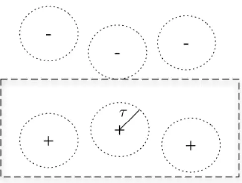
First, in order to use the notion of margin, we need to define some measure of distance, or similarity, between examples. To formalize this notion, we assume for simplicity that all predicates in the language are unary and that examplesϕ(a)_∧C(a) are such that ϕ(a) is a conjunction of literals, i.e. ϕ(a) is of the form p1(a)∧. . .∧pk(a)∧ ¬pk+1(a)∧. . .∧ ¬pn(a). In that case, the only variable in a predicate stands for an example identifier, and hence for our purposes here we can actually consider these unary predicates as atomic propositions. Simplifying, we will denote by ϕ the propositionalized version of ϕ(a), i.e. ϕ = p1 ∧. . .∧pk∧ ¬pk+1 ∧. . .∧ ¬pn. This is indeed the case in the example described in Section 5. We will further assume the set _P of unary predicates (now propositional variables) we work with is finite.

Let Ω =_{w:_{P → {}0,1_}}be the space of possible worlds. Given a propo-sitional formula ϕ, we will denote by [ϕ] the set of possible worlds satisfying the formula ϕ (according to classical propositional logic). We assume there is a distance function δ : Ω_×Ω_→R+_{. The intuition is that δ(w, w}0₎

evalu-ates how far or different two worlds w and w0 are: δ(w, w0) = 0 means that

w = w0, 0 < δ(w, w0) < 1 means that w resembles to w0 to some degree. A usual choice forδ, among others (see e.g. [17, 18]), is the Hamming distance, that counts the number of elements of _P over which two worlds differ.

Given such a distance function δ on the set of possible worlds Ω, the distance between two propositional formulas built form _P can be measured by the distance between the corresponding sets of possible worlds, using the well-known Hausdorff distance derived from δ: δH(ϕ, ψ) = max(Iδ(ϕ |

ψ), Iδ(ψ |ϕ)), where Iδ(ϕ|ψ) = max w∈[ψ] min w0_∈[ϕ]δ(w, w 0₎

Now, given a set of examples ∆, a distanceδ and a threshold τ _∈R+_{, we} can consider an expanded set of examples ∆∗_τ where for eachϕ(a)_∧C(a)_∈∆ (resp. ϕ(b)_{∧ ¬}C(b)_∈∆) we include all those additional fictitious examples

ψ(a0)_∧C(a0) (resp. ψ(b0)_{∧ ¬}C(b0)), such that the distance betweenψ and ϕ

is at most τ, i.e. such that δH(ϕ, ψ)≤τ.

Given an inductive theoryT _⊆IRK(∆), we say thatT isvalid to the level

+ + ₊

-τ

Figure 1: Margin based on similarity measure δH.

∆∗_τ must be consistent). We assign a preference degree τ to an inductive theory T, noted Pref(T) = τ, when τ is the maximum for which T is still an inductive theory of IRK(∆∗_τ) (i.e. Pref(T) is the maximum degree to which T is valid). This induces a natural preference over inductive theories:

T _≥∆,K T0 ⇔ Pref(T) ≥ Pref(T0). Moreover, according to Definition 9, a preferred inductive theory T is one such that there is no other inductive theory T0 _⊆IRK(∆) such that T0 >∆,K T.

Notice that, in the present setting, a preferred inductive theory T max-imizes the margin according to the distance δH. As shown in Fig.1, the reason is that ∆∗_τ is expanding as much as possible around all positive ex-amples ϕ(a)_∧C(a) and negative examples ϕ(b)_{∧ ¬}C(b) without T covering any fictitious example of the opposite sign.

4.3. Exemplification

Let us now illustrate the use of preferences by continuing the exemplifi-cation started in Section 3.3.

Let us consider again the inductive theories used before:

T1 = {r1} ⊆ IRK(∆), T2 = {r4} ⊆ IRK(∆) and T3 = {r1, r4} ⊆ IRK(∆), and consider a new inductive theory T4 ={r1, r5, r6}, where:

r5 := (∀x)(hair(x)∧f ourlegged(x)→m(x))

r6 := (∀x)(milk(x)∧f ourlegged(x)→m(x))

Given a functionsize(_·), counting the symbols in a formula (ignoring paren-thesis), the size of an inductive theory is simply the sum of the sizes of its rules. Thus we have: size(r1) = 10, size(r4) = 7, size(r5) = 10,

size(T4) = 30. Using the parsimony preference we have: T2 ≥∆,K T1 ≥∆,K

T3 ≥∆,K T4. In fact, there is no other inductive theory with size smaller than 7, and thus T2 is a preferred inductive theory. Since T2 is also minimal, it is actually an ideal inductive theory.

Notice, however, that if we were to use margin maximization as the pref-erence criterion, with the Hamming distance, T2 would not be preferred, since it is only valid to the level 0. In fact, the margin preference degrees of these inductive theories are Pref(T1) = 0, Pref(T2) = 0, Pref(T3) = 0, Pref(T4) = 1 and, thus, T4 would be preferred to the others.

5. Induction and Argumentation

One of the main advantages of having a logical model of induction is that it allows an easy integration of inductive reasoning with other forms of logical reasoning. In order to illustrate its benefits, this section presents a model of multiagent ICL obtained by directly integrating our inductive consequence relation with computational argumentation. In this integration, argumentation is used to model the communication between agents, and ICL models their internal learning processes.

For the sake of simplicity of presentation, we will consider a multiagent system scenario with two agents Ag1 and Ag2 having a same target con-cept C. However, as shown in A, our main theoretical result applies to the more general case of an arbitrary number of agents. We make the following assumptions:

1. The background knowledge K of both agents is the same2,

2. The set of rules _Lr and the set of examples Le are defined as before (see Section 3).

3. Each agent has a set of examples ∆1,∆2 ⊆ Le such that ∆1 ∪∆2 is consistent.

The goal of each agent Agi is to induce an inductive theory Ti such that

Ti ⊆ IR(∆1∪∆2) and that constitutes an inductive theory w.r.t. ∆1∪∆2. We will call this problem multiagent ICL.

2_{For simplicity, since both agents shareKandC, in the rest of this paper we will write}

IR(∆) rather than IRK(∆), and just say inductive theory, instead of saying inductive theory of C.

For this purpose, a na¨ıve approach would be to have both agents sharing their complete sets of examples; however, that might not be always feasible for a number of reasons, like cost or privacy. In this section, we will show that by sharing some of the rules they have induced from examples (rather than all of their examples), two agents can also solve the multiagent ICL problem. Let us start presenting our computational argumentation framework.

5.1. Computational Argumentation

We will follow Dung’s abstract argumentation formalization [19] and de-fine an argumentation framework as a pair _A = (Γ,), where Γ is a finite set of arguments, and is an attack relation.

Given two arguments,randr0, we writerr0to represent thatrattacks

r0. Moreover, if both rr0 and r0 r we say that r blocks r0.

As in any argumentation system, the goal is to determine whether a given argument is defeated or not according to a given semantics. In our case we will adopt the semantics based on dialectical trees [20, 21] explained below:

Definition 11. (Argumentation Line) Given an argumentation frame-work _A = (Γ,) and r0 ∈ Γ, an argumentation line in A rooted in r0 is a sequence: λ=_hr0, r1, r2, . . . , rki such that:

1. ri+1 ri (for i≤k),

2. if ri+1 ri and ri blocks ri−1 then ri 6ri+1. The argument rk is called the leaf node of λ.

Additionally, for the purposes of ICL, we will assume that the attack relation has no cycles (which is the case for the definition of attack we will introduce later in this paper, Definition 12), and hence there are no repeated arguments in an argumentation line. Consequently, argumentation lines are always finite by construction. The set Λ(r0) of maximal argumentation lines rooted inr0 are those that are not subsequences of other argumentation lines rooted in r0. Clearly, Λ(r0) can be arranged in the form of a tree, where all paths from the root to the leaf nodes exactly correspond to all the possible maximal argumentation lines rooted in r0 that can be constructed in the given argumentation framework. In order to decide whetherr0 is defeated in

A, the nodes of this tree are marked U (undefeated) or D (defeated) according to the following (cautious) rules:

2. Each inner node is marked U iff all of its children are marked D, oth-erwise it is marked D.

Therefore, the arguments in the argumentation framework _A will be ei-ther undefeated or defeated according to their marking, as follows:

Undefeated: U(_A) =_{r _∈Γ_|r is marked U in the tree Λ(r)_}

Defeated: D(_A) = _{r_∈Γ_|r is marked D in the tree Λ(r)_}. 5.2. Argumentation-based Induction

Induction and argumentation can be integrated through the notion of argumentation-consistent induction. While induction was defined with re-spect to a set of observations ∆, argumentation-consistent induction will be defined with respect to a set of observations ∆, and a set of arguments Θ. The essential idea is that we consider arguments to be rules, i.e. Θ_{⊆ L}r (an example can also be used as an argument through its corresponding lifted rule, see the reflexivity property in Proposition 1). Therefore, in the rest of this paper, we will use the terms “rule” and “argument” interchangeably.

Given that arguments will be rules, we can now define the attack relation

between rules as follows.

Definition 12. (Attack)Given two rulesr, r0 _∈Γ, an attack relationr r0

holds whenever:

1. r = (_∀x)(α(x)_→`(x)), 2. r0 = (<sub>∀</sub>x)(β(x)<sub>→ ¬</sub>`(x)), and 3. K _`(_∀x)(α(x)_→β(x)).

where _¬`=<sub>¬</sub>C when `=C and _¬`=C when `=_¬C.

Argumentation-consistent induction consists of inducing rules that agree with both ∆ (i.e. not covering negative examples present in ∆) and Θ (i.e. not being defeated by the arguments in Θ).

Definition 13. (Argumentation-consistent Inducible Rule)

A rule r _∈ IR(∆) is argumentation-consistent with respect to a set of arguments Θ if r_∈U(_A), where _A= (Θ_∪IR(∆),).

The set of all the argumentation-consistent rules induced is AIR(∆,Θ) = IR(∆)_∩U(_A).

Now we can define argumentation-consistent inductive theories.

Definition 14. (Argumentation-consistent Inductive Theory) An argumentation-consistent inductive theory T, with respect to ∆ and a set of arguments Θ, is an inductive theory of ∆ such that T _⊆AIR(∆,Θ).

In the multiagent context starting in the next section, the goal of an agent is to build an argumentation-consistent inductive theory, where such theory will be composed by rules that have not been defeated by a set of arguments Θ coming from another agent.

6. Argumentation-consistent Induction in Multiagent Systems

Let us now show how the notion of argumentation-consistent induction can be used to model induction in a scenario with two agents. The main idea is that agents induce rules from the examples they know, and then they share them with the other agent. Rules received from the other agent are added into the own agent’s argumentation framework to update her argumentation-consistent induced rules. Thus, in addition to the set of examples ∆i, each agentAgihas an individual argumentation frameworkAi, containing both (1) the set of inducible rulesIR(∆) inducted byAgi and (2) the set of arguments Θ received from another agent.

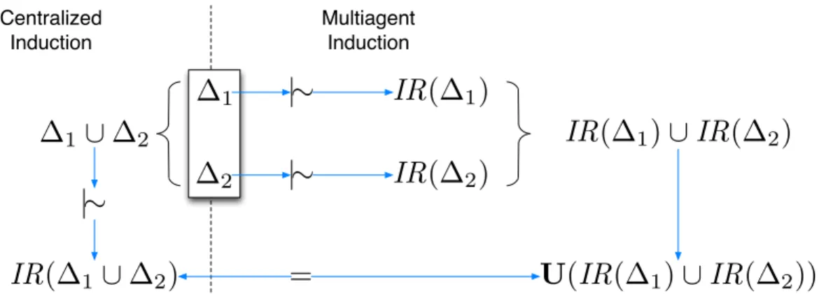
Let us now prove that two agents communicating their induced rules and performing argumentation using the kind of attack in Definition 12 would obtain the exact same set of inducible rules as a single agent knowing the examples known to both agents.

Since the attack relation between rules is always the same, in the following we will simply write U(Γ) instead of U(_A) to denote the set of undefeated rules of the argumentation system _A = (Γ,).

Theorem 1. (Argumentation-consistent Induction) U(IR(∆1)∪IR(∆2)) =IR(∆1∪∆2).

Proof. Notice that by definition U(IR(∆)) = IR(∆); consequently, we have AIR(∆,IR(∆)) =IR(∆).

First, we prove that IR(∆1 ∪∆2) ⊆ U(IR(∆1) ∪ IR(∆2)). Let r ∈ IR(∆1∪∆2) thenr =α →C covers a positive example of ∆1∪∆2 and does not cover any negative example of ∆1 ∪∆2. W.l.o.g., assume the covered positive example is from ∆1. Then r∈ IR(∆1). Suppose there exists a rule

1

[

|⇠

IR

(

)

IR

(

)

IR

(

)

[

IR

(

)

U

(

IR

(

)

[

IR

(

))

IR

(

[

)

|⇠

|⇠

=

Figure 2: Achieving multiagent induction by combining inductive reasoning and compu-tational argumentation.

r0 =β _{→ ¬}C _∈IR(∆1)∪IR(∆2) such thatr0 r, i.e. such thatK `β →α. It is clear that r0 _6∈ IR(∆1), hence assume that r0 ∈IR(∆2). This means r0 covers a negative example δ− _∈ ∆2, but if r0 covers it, r must cover δ− as well, contradiction.

Second, we prove that IR(∆1 ∪∆2) ⊇ U(IR(∆1)∪ IR(∆2)). Let r ∈

U(IR(∆1)∪IR(∆2)). W.l.o.g., assume r ∈IR(∆1). Then r =α→C covers a positive example of ∆1 and does not cover any negative example of ∆1. Assume also, looking for a contradiction, thatr_6∈IR(∆1∪∆2). Since we have assumed thatr _∈IR(∆1), this means thatrcovers a negative example of ∆2. This negative example can be specialized to a rule r0 = β _{→ ¬}C _∈ IR(∆2) such that K _` β _→ α. Since r0 is the specialization of an example in ∆2 and ∆1 ∪ ∆2 is consistent, the rule r0 is undefeated. Consequently, r 6∈

U(IR(∆1)∪IR(∆2)), which contradicts our original assumption. Therefore we can conclude IR(∆1∪∆2)⊇U(IR(∆1)∪IR(∆2)).

The previous theorem shows that, given two agents, Ag1 and Ag2, each one with sets of examples ∆1 and ∆2 respectively, they can induce the same set of rules either by sharing their induced rules IR(∆1) and IR(∆2) and then using argumentation, or by exchanging all of their examples and then using induction. This equivalence is illustrated in Figure 2, that shows two equivalent approaches to obtain an inductive theory w.r.t ∆1∪∆2: centralized induction (on the left hand side), and argumentation-consistent induction (on the right hand side). In A of this paper, we show how this result applies to the more general case of an arbitrary number of agents.

since a) they can be very large, and b) given the reflexivity property,IR(∆i) contains ∆i. Nevertheless, Theorem 1 shows that theoretically, the problem of multiagent ICL can be modeled using individual induction plus argumen-tation. In fact, if the purpose is finding inductive theories, not all arguments in the IR(∆i)’s need to be exchanged. Section 7 presents a dialogue game that finds an inductive theory w.r.t. ∆1∪∆2 using the same theoretical idea as used in Theorem 1, but focusing on exchanging a smaller subset of rules. However, let us first illustrate the concepts of argumentation-consistent induction described in this section with an exemplification.

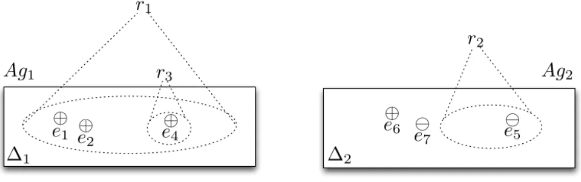
6.1. Exemplification

Consider two agents, Ag1 and Ag2, knowing a set of examples ∆1 = {e1, e2, e4} and ∆2 = {e5, e6, e7}. Here, e1, e2 and e3 are the three examples used in Section 3.3, and the new four examples (e4 is a sealion, e5 is a seasnake, e6 is a platypus, and e7 is a chicken) are defined as:

e4 := hair(a4)∧milk(a4)∧aquatic(a4)∧predator(a4)∧toothed(a4) ∧backbone(a4)∧breathes(a4)∧f ins(a4)∧twolegged(a1) ∧tail(a4)∧catsize(a4)∧m(a4)

=ϕ4(a4)∧m(a4)

e5 := aquatic(a5)∧predator(a5)∧toothed(a5)∧backbone(a5) ∧venomous(a5)∧f ins(a5)

∧tail(a5)∧ ¬m(a5) =ϕ5(a5)∧ ¬m(a5)

e6 := hair(a6)∧eggs(a6)∧milk(a6)∧aquatic(a6)∧predator(a6) ∧backbone(a6)∧breathes(a6)∧f ourlegged(a6)∧tail(a6) ∧catsize(a6)∧m(a6)

=ϕ6(a6)∧m(a6)

e7 := f eathers(a7)∧eggs(a7)∧airborne(a7)∧backbone(a7)∧ breathes(a7)∧twolegged(a7)∧tail(a7)∧ ¬m(a7)

=ϕ7(a7)∧ ¬m(a7)

Thus, ∆1 contains three positive examples (e1,e2and e4) and no negative example, and ∆2 contains two negative examples (e5 ande7) and one positive example (e6). Let us now consider some of the rules that the agents can induce from those examples. For instance, two of the rules that Ag1 can induce are r1, r3 ∈IR(∆1) below:

r

r

Ag

Ag

e

e

e

e

e

e

r

Figure 3: Two agents,Ag1andAg2, knowing different sets of examples, and some sample rules that can be induced from them.

r1 := (∀x)(backbone(x)→m(x))

r3 := (∀x)(backbone(x)∧toothed(x)∧twolegged(x)→m(x)) AgentAg2 can induce the rule r2 ∈IR(∆2):

r2 := (∀x)(backbone(x)∧toothed(x)→ ¬m(x))

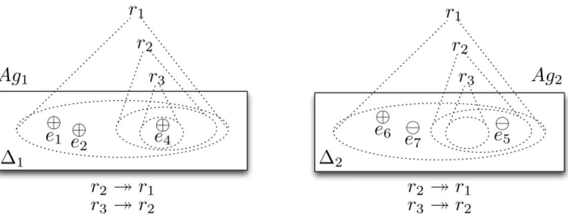
When the two agents perform induction in isolation, no issues are found with those three rules, as shown in Figure 3. However, let us consider now the situation where agent Ag1 communicates r1 and r3 to Ag2, and Ag2 communicates r2 to Ag1. In this situation, according to Definition 12, the following attacks hold: r2 r1 and r3 r2.

Let us first consider Ag1, who, in addition to its inducible rules IR(∆1), now has access to the set of rules Θ2→1 = {r2}. Now, to perform argumentation-consistent induction, Ag1 assesses which are the rules that are both inducible from ∆1 and consistent with Θ2→1. For that purpose,

Ag1 constructs the argumentation frameworkA1 = (IR(∆1)∪ {r2},). It is easy to verify that, since r2 is attacked by r3, and r3 is not attacked by any other rule, r2 is defeated. Thus, bothr1 andr3 are argumentation-consistent inductions and belong to AIR(∆1,Θ2→1). Therefore, knowing r2 does not change the set of inducible rules of Ag1, even if r2 attacks r1 (see Figure 4). Now, considering agentAg2, in addition to its inducible rulesIR(∆2), now

Ag2 has access to the set of rules Θ1→2 = {r1, r3}. Similarly as before, to perform argumentation-consistent induction,Ag2 assesses which are the rules that are both inducible from ∆2 and consistent with Θ1→2. Ag2 constructs the argumentation framework _A2 = (IR(∆2)∪ {r1, r3},). In this case, the rule r2, induced by Ag2 is defeated (because it is attacked by r3, which is

r

r

Ag

Ag

e

e

e

e

e

e

r

r

r

r

r

⇣

r

r

⇣

r

r

⇣

r

r

⇣

r

Figure 4: The same two agents from Figure 3, after they communicate some rules.

not attacked by any other rule), and thusr2 6∈AIR(∆2,Θ1→2). Thus, in this case, knowing r1 and r3 changes the the set of inducible rules of Ag2.

7. Reaching Inductive Theories in Multiagent Concept Learning

While Theorem 1 shows that it is possible to solve the problem of multi-agent ICL using individual induction plus argumentation, this section shows that when agents want to just agree on a single inductive theory, it is not necessary, in general, to exchange all of their induced rules. This section presents a dialogue game [22] through which two agents can solve the mul-tiagent ICL problem by communication, specifically by exchanging some of the rules they induced from examples. To define the dialogue game, we need to define an interaction protocol, including the types of messages that agents are allowed to use, and the conditions under which types of messages can be exchanged. The dialogue game is defined for two agents Ag1 and Ag2, each of which has an individual set of examples ∆1, ∆2, and consists of a series of rounds. At each round t of the dialogue game, each agentAgi holds a current inductive theory, T_it, that is revised after each round. When the game terminates, both agents reach a common inductive theory with respect to ∆1∪∆2.

During the dialogue game, agents communicate to each other rules in-duced from their examples. Through this rule exchange, an agent Agi may attack the inductive theory Tt

j of the other agent Agj if it is not consistent with ∆i.

At the end of each round t, an agent Agi knows the following six pieces of information, namely (∆i, Tit, Tjt,Θti→j,Θtj→i,Ati), where:

1. ∆i is the set of examples known to Agi.

2. T_it is the current inductive theory w.r.t ∆i that agentAgi is holding. 3. Tt

j is the current inductive theory w.r.t ∆j that the other agent is holding.

4. Θt_i→j is the set of arguments (rules) that agent Agi has sent to Agj up to the round t. Notice that Θt

i→j ⊆IR(∆i).

5. Θt_j→i is the set of arguments (rules) that agent Agi has received from

Agj up to the round t. 6. _At

i = (IR(∆i) ∪Θjt→i,) is the argumentation framework for Agi; notice that the set of arguments is composed of the rules inducible by

Agi plus the arguments sent by the other agent Agj.

Let us now provide some auxiliary definitions, before we introduce the dia-logue game interaction protocol.

Definition 15. (Defeaters of a rule)

Given an argumentation framework _A = (Γ,), and a defeated argument

r _∈D(_A), the set of defeaters of r is:

Defeaters(r,_A) =_{r0 _∈Γ_|r0 r and r0 _∈U(_A)_} That is to say, the set of undefeated arguments that attack r.

Definition 16. (Defeated Arguments From Communication)

Given the set of argumentsΘt

j→i communicated byAgj toAgi, the set of those received arguments that are defeated according toAgi isDtj→i =D(Ati)∩Θtj→i. Using the previous definitions, we can now present the dialogue game through which two agents Ag1 and Ag2 can find an inductive theory w.r.t. ∆1∪∆2.

Before the first round, at t = 0, the two agents are assumed to hold initial inductive theories T₁0 _⊆IR(∆1) and T20 ⊆ IR(∆2) w.r.t. ∆1 and ∆2 respectively. Moreover, we assume each agent has communicated its own inductive theory to the other agent, and thus:

Θ0

Consequently, the initial argumentation systems of the agents are set to:

A0

1 = (IR(∆1)∪Θ02→1,) and A02 = (IR(∆2)∪Θ01→2,).

Then, at each round t, starting at t = 1, each agent Agi computes the new values of the tuple (T_it,Θt_i→j,Ati), based on the values at the previous round (T_it−1,Θ_it_→−1_j,_Ait−1). Notice that ∆i does not change and Tjt and Θtj→i are computed by the other agent.

Actually, each roundt_≥1 of the protocol is divided in five simple steps: generate attacks, send attacks, update inductive theories, send updated in-ductive theories, and update state. The process ends when no agent generates new attacks. In more detail, a round t of the protocol is as follows:

1. Generate Attacks: Agi generates a set of attacks Rti by selecting a single argument (whichever) r0 _∈ Defeaters(r,_Ait−1) for each r _∈Dt_j−_→1_i

i.e. Agi selects one attack for each argumentr sent by the other agent that is defeated according to Agi.

2. Send Attacks: Each agent Agi sends Rti to the other agent.

If _Rt_i = _Rt_j = _∅, then the process terminates, since this means that the current theories held by each agent (T_it−1 and T_jt−1) are acceptable for the other agent (no attack can be found). Otherwise the protocol proceeds to the next step.

3. Update Inductive Theories: Each agent Agi generates a new argumentation-consistent inductive theory Tt

i ⊆ AIR(∆i,Θjt−→1i ∪ Rtj) such that (T_it−1_∩U(_Bt_i−1))_⊆Tt

i, whereB t−1

i = (IR(∆i)∪Θtj−→1i∪Rtj,) —i.e. the new theory T_it contains all the undefeated rules from T_it−1

taking into account the attacks received, and replaces the rules that were defeated in T_it−1 by new rules.

4. Send Updated Inductive Theories: Each agent Agi sends Tit to the other agent.

5. Update State: the set of arguments received by each agent is in-creased accordingly: • Θt 1→2 = Θ t−1 1→2∪ Rt1∪T1t • Θt 2→1 = Θ t−1 2→1∪ Rt2∪T2t

both agents update their argumentation frameworks:

• At

• At

2 = (IR(∆2)∪Θt1→2,)

And new round t+ 1 starts by going back to the first step.

When the process terminates, both agents have a common and agreed argumentation-consistent inductive theory, namely T∗ =Tt

1 ∪T2t.

The reason is that, when the process terminates, if the set ∆1 ∪∆2 is consistent, then each agent Agi has an argumentation-consistent inductive theory Tt

i w.r.t. ∆i that is also consistent with the examples in ∆j. Never-theless, T_it might not be an inductive theory w.r.t. ∆j, since there might be examples in ∆j not covered by Tit. However, their union T

∗ _=Tt

1 ∪T2t is an inductive theory w.r.t. the examples in ∆1∪∆2 and, since both agents know

T₁tandT₂t, both agents can haveT∗ as a common and agreed argumentation-consistent inductive theory w.r.t. ∆1∪∆2, as the following theorem proves.

Theorem 2. If the set ∆1 ∪∆2 is consistent, the previous process always ends in a finite number of roundst, and when it ends, T₁t_∪T₂t is an inductive theory w.r.t. ∆1∪∆2.

Proof. First, let us prove that the final theories (Tt

1 and T2t) are consistent with ∆1∪∆2. For this purpose we will show that the termination condition (Θt

1→2 = Θ t−1

1→2 and Θt2→1 = Θ t−1

2→1) implies that the argumentation-consistent inductive theoryTt

i found by agentAgi at the final roundt has no counterex-amples in either ∆1 nor in ∆2.

Let us assume that there is an exampleak ∈∆1which is a counterexample of a rule r _∈ Tt

2. Because of the reflexivity property, there is a rule rk ∈ IR(∆1) which corresponds to that example. Since ∆1 ∪∆2 is consistent, there is no counterexample of rk, and thus rk is undefeated. Since rk r by assumption, r would have been defeated, and therefore rule r could not be part of any argumentation-consistent inductive theory generated by Ag2. The same reasoning can prove that there are no counterexamples of Tt

1 in ∆1∪∆2.

Since T₁t and T2 are inductive theories w.r.t. ∆1 and ∆2 respectively, it follows from the above that Tt

1 ∪T2t is an inductive theory w.r.t. ∆1 ∪∆2 because it has no counterexamples in ∆1∪∆2, and every example in ∆1∪∆2 is explained at least by one rule in T₁t or in T₂t.

Finally, the process has to terminate in a finite number of steps, since, by assumption, IR(∆1) and IR(∆2) are finite sets, and the sets Θt1→2 and Θt_2→1 grow at least with one new argument at each round; however, since

Θt

i→j ⊆IR(∆i), there is only a finite number of new arguments that can be added to Θt_i→j before the termination condition holds.

Thus, we have shown that the inductive theories achieved by argumentation-consistent induction are sound. Theorem 1 has shown that the set of inductive theories that can be reached through sharing examples is the same as the set of inductive theories that can be reached by sharing induced rules and then performing argumentation-consistent induction. Fur-thermore, Theorem 2 shows that it is possible to reach one of those inductive theories by using a simple dialogue game that does not require in general the exchange of all the induced rules made by an agent. As a consequence, cen-tralizing all examples into a single inductive process is no longer imperative, at least in ICL, since induction followed by argumentation is a viable option. The process to find a multiagent inductive theory can be seen as composed of three mechanisms: induction, argumentation and belief revision. Agents use induction to generate general rules from concrete examples, they use argumentation to decide which of the rules sent by another agent cannot be defeated, and finally they perform belief revision when they change their inductive theories in light of the arguments sent by another agent. The belief revision process is embodied in the way the set of undefeated rules U(_At_i) changes from round to round, which also determines how an agent’s inductive theory changes in light of the arguments shared by the other agent.

A particular implementation of this integration model is the A-MAIL framework [9], where two agents perform induction on separate example sets and engage in argumentation until they reach individual inductive theories that are consistent with their example sets. The A-MAIL framework offers a particular realization of three mechanisms of induction, argumentation and belief revision. The need of having an argumentation-consistent inductive process is met byABUI(Argumentation-based Bottom-Up Induction), a new inductive method that finds inductive rules consistent with the set of unde-feated rules at any step of the argumentation process.

7.1. Exemplification

Let us assume we have two agents,Ag1 andAg2 and let ∆1 ={e1, e2, e3} (containing the three examples used in Section 3.3, an aardvark, an antelope and a bass), and ∆2 ={e4, e6, e7} (containing some of the examples used in Section 6.1, a sealion, a platypus, and a chicken). Now, the two agents want

to find a common inductive theory of the concept mammal, represented by the unary predicate m. Let us explain the process.

Before the protocol starts, att= 0, each agent has individually found an inductive theory:

T₁0 =_{(_∀x)(breathes(x)_→m(x))_}, and

T0

2 ={(∀x)(aquatic(x)→m(x))}.

Intuitively, since all the positive examples of mammal known toAg1 are land animals, and all the negative ones are not, Ag1 has induced that breathing is enough to characterize a mammal. A similar situation has occurred with

Ag2, who has find by induction that beingaquatic is enough to characterize a mammal, since it happens that the only two examples of mammals Ag2 knows are aquatic.

Moreover, att= 0, each agent has communicated to the other agent their individually found inductive theories and build their initial argumentation systems, and thus:

Θ0

1→2 =T10, and Θ02→1 =T20;

A0

1 = (IR(∆1)∪Θ02→1,) and A02 = (IR(∆2)∪Θ01→2,). The protocol then proceeds as follows.

Round t= 1.

1. Agents proceed by generating attacks against the rules they have re-ceived they believe are defeated.

• Since the rule (_∀x)(aquatic(x) _→ m(x)) generated by Ag2 is defeated according to Ag1, Ag1 selects one attack to defeat it:

R1

1 ={(∀x)(aquatic(x)∧ ¬hair(x)→ ¬m(x))};

• Since the rule (_∀x)(breathes(x) _→ m(x)) generated by Ag1 is defeated according to Ag2, Ag2 selects one attack to defeat it:

R1

2 ={(∀x)(breathes(x)∧f eathers(x)→ ¬m(x))}; 2. These attacks are sent to each other.

• Due to the attacks recieved, Ag1 updates its inductive theory by removing all the defeated arguments, and replacing them by new undefeated arguments, and generates: T₁1 = _{(_∀x)(hair(x) _→

m(x))_}.

• Analogously, Ag2 updates its inductive theory by removing all the defeated arguments, and replacing them by new undefeated arguments, and generates: T1

2 ={(∀x)(milk(x)→m(x))}. 4. These theories are sent to each other.

5. Agents update their states:

• Θ1

1→2 = Θ01→2∪ R11∪T11; Θ12→1 = Θ02→1∪ R12∪T21;

• A1

1 = (IR(∆1)∪Θ12→1,),A21 = (IR(∆2)∪Θ11→2,) Round t= 2.

1. Agents should try now to generate attacks, but since the arguments sent in the previous round _R1₁ and _R1₂ are undefeated in the argumentation systems _A1

2 and A11 respectively, no new attacks can be generated and the protocol ends.

As a result, both agents have reached inductive theories T1

1 and T21 that are consistent with the whole set of examples of both agents ∆1∪∆2 (i.e. each theory has any counterexample neither in ∆1 nor in ∆2). Theorem 2 guarantees that

T∗ =T₁1_∪T₂1 =_{(_∀x)(hair(x)_→m(x)),(_∀x)(milk(x)_→m(x))_} is a common and agreed argumentation-consistent inductive theory. Notice that this result is reached without exchanging any example, and exchanging a small amount of inducible rules.

8. Related Work

Peter Flach [1] introduced a logical analysis of induction, focusing on hypothesis generation. In Flach’s analysis, induction was studied on the meta-level of consequence relations and focused on different properties that may be desirable for different kinds of induction. In this paper we cover both hypothesis generation and hypothesis selection, but we focus in a limited form of induction, namely inductive concept learning, extensively studied in

machine learning. A direct difference between Flach’s work and the research presented in this paper is that we impose strong syntactical constraints on our inductive consequence relation (from sets of examples to rules), in order to focus on the specific machine learning problem of inductive concept learning, whereas the work of Peter Flach, no restrictions were applied, in order to study the soundness and completeness of sets of meta-level properties of inductive consequence relations. Appendix B offers an in-depth comparison of some properties of our consequence relation with some of Flach’s meta-level properties.

A refinement of Flach’s consistency-based confirmation using Hempel’s direct confirmation was studied in [4]. The authors proposed that inductive generalization can be modeled as a deductive process given a completion technique, which captures inductive assumptions, such as “every unknown individual is similar to the known ones.” The difference with our work is that, albeit restricted to the particular task of ICL, we propose a specific non-monotonic logic consequence relation, instead of resorting to a completion technique.

Related to the work of Flach is that of DelGrande [3], where he studied the algebra of hypotheses that can be formed by induction from sets of exam-ples. In the same way as Flach, DelGrande limited his study to hypothesis generation, and considered that his model is a restriction with respect to the general problem of induction, where induction as such plays the limited role of proposing an initial set of hypotheses, which is later refined using deductive techniques.

Also related is the work of Datteri et al. [2], where induction (in machine learning) was understood as a deductive process; Dateri et al. modeled a typ-ical process of a machine learning inductive algorithm in several steps, and provided a logical model for each step (that they call “deductive”). The final argument was that machine learning inductive algorithms are then “induc-tionless,” as every step in the process is a logical inference. Our approach, a non-monotonic logical model of the whole process of an inductive algorithm, clarifies the nature of inductive concept learning: it is a form of defeasible (i.e. non-deductive) reasoning, similar (albeit not identical) to other forms of defeasible reasoning modeled by non-monotonic logic.

Concerning the integration of inductive reasoning with other forms of log-ical reasoning, Michalski [23], in his Inferential Theory of Learning, started a unified characterization of all forms of inference (deduction, analogy, induc-tion, etc.) and defined knowledge transmutation operators. However, those

operators were only illustrated with examples, and never completely formal-ized. In this paper, we have taken on a smaller task: instead of trying to formalize all types of inference, we have focused on a very specific form of inference (inductive generalization), and, in this way, we have man