Dynamic graphics of parametrically linked multivariate methods used in compositional data analysis

Dynamic graphics of parametrically linked multivariate methods used

in compositional data analysis

Michael Greenacre

Universitat Pompeu Fabra, Barcelona, Spain; Email: [email protected]

NOTE TO THE READER

This working report contains dynamic graphics which can be viewed directly in the

PDF file, using Acrobat Reader 6. Each figure shows four selected images from the

graphics video sequence – clicking on the figure (inside the light blue frame) will start

the video.

The quality of the video is not as good as the original and I am investigating how to

improve it. But I have also posted the videos on the web-page:

www.econ.upf.edu/

~michael/

CodaWeb.htm

where they can be alternatively viewed in a higher quality.

Do not be concerned by

the warning messages when you open this web-page.

I believe this is the first time that a UPF working paper contains dynamic graphic

content – any feedback or advice in this regard will be welcome.

This paper forms my presentation at CODAWORK 2008, the biennial international

meeting on compositional data analysis held at the University of Girona:

Dynamic graphics of parametrically linked multivariate methods used in

compositional data analysis

Michael Greenacre

Universitat Pompeu Fabra, Barcelona, Spain; [email protected]

Abstract

Many multivariate methods that are apparently distinct can be linked by introducing one or more parameters in their definition. Methods that can be linked in this way are correspondence analysis, unweighted or weighted logratio analysis (the latter also known as "spectral mapping"), nonsymmetric correspondence analysis, principal component analysis (with and without logarithmic transformation of the data) and multidimensional scaling. In this presentation I will show how several of these methods, which are frequently used in compositional data analysis, may be linked through parametrizations such as power transformations, linear transformations and convex linear combinations. Since the methods of interest here all lead to visual maps of data, a "movie" can be made where where the linking parameter is allowed to vary in small steps: the results are recalculated "frame by frame" and one can see the smooth change from one method to another. Several of these "movies" will be shown, giving a deeper insight into the similarities and differences between these methods.

Keywords: compositional data; contingency tables; correspondence analysis; logratio

transformation; singular value decomposition; spectral map; weighting.

1 Introduction

In a previous paper at CODAWORK 2005, Greenacre & Lewi (2005a) clarified and demonstrated the following:

• Principal component analysis of compositional data, as originally proposed by Aitchison (1980, 1983) – based on log-ratios – is an unweighted version of what Lewi (1976) defined as the “spectral map”. It is the biplot based on this unweighted form that was studied by Aitchison and Greenacre (2002).

• The spectral map weights the rows and columns of a positive data matrix in the same way as in correspondence analysis (CA) – for a recent account see Greenacre (2007). That is, the weights are the relative row and column margins (called masses in CA), which for compositional data would be: (i) equal weighting for all rows (samples) and (ii) weights equal to the mean composition for columns (components).

• The effect of the weighting can lead to dramatic improvements in the analysis of compositional data, because the influence of high log-ratios often present in rare components is reduced. The weighting also gives the analysis distributional equivalence – the cornerstone property of CA (Greenacre & Lewi, 2005b, to appear in 2008). In this respect weighted LRA has better theoretical properties than CA, and also has the advantage of being able to diagnose equilibrium models, but suffers the disadvantage of complications in the presence of data zeros.

To distinguish between the different PCA/biplot variants of log-ratio analysis (LRA), the terms unweighted LRA and weighted LRA were introduced, the latter being the spectral map. At that time we looked at CA and LRA, weighted and unweighted, as different methodologies sharing the singular-value decomposition (SVD) as algorithmic engine for dimension-reduction. Since then Greenacre (2007, to appear in 2008) showed that CA and LRA were more closely linked, thanks to the Box-Cox transformation (1/α) (xα–1). The “trick” was to realize what arguments x to subject to the Box-Cox transformation in order to link the methods by a power transformation. The main results are as follows, where N denotes the original matrix of compositional data (see Greenacre (2007) for the technical details):

Power family 1: Pre-transform the matrix N, by the power transformation n_ij(α) = n_ijα. In the CA of this matrix the row and column masses change with α. In the CA algorithm multiply by (1/α) the double-centred matrix on which weighted singular value decomposition (SVD) is performed.

Power family 2: Pre-transform the matrix Q of contingency ratios (i.e., the observed values n_ij divided by their “expected values” based on the margins) by the power transformation q_ij(α) = q_ijα . The original masses r_i and c_j are maintained constant throughout, both in double-centring and in the weighted SVD. Again the matrix on which the SVD is performed is multiplied by (1/α).

In power family 2, whether we double-centre (1/α) q_ijα or (1/α) (q_ijα–1) makes no difference at all, because the constant term will be removed by double-centring. Hence, the analysis in this case amounts to the Box-Cox transformation of the contingency ratios:

(

)

α qij (1)

which converges to log(q_ij) as α→0. Thus power family 2 converges to weighted LRA as α→0.

In power family 1, we are also analysing contingency ratios of the form (1/α) q_ijα , or (1/α) (q_ijα–1), but then the ratios as well as the weights and double-centring are all with respect to row and column masses that are changing with α. At the limit as α→0, these masses tend to constant values, i.e. 1/I for the rows and 1/J for the columns; hence the limiting case of power family 1 is the analysis of the logarithms with constant masses, or unweighted LRA.

The consequence of the above results is that CA and LRA, weighted and unweighted, are part of the same family, parametrized by the power coefficient α. When α = 1 the analysis is CA in both cases, but when

α→0 we have unweighted LRA in the first case and weighted LRA (spectral map) in the second. The objective of this paper is to present some illuminating dynamic graphics that show smooth transitions between CA and both forms of LRA as well as between unweighted and weighted LRA, which can be achieved simply by changing the weights in a smooth way. We will use two well-known examples: the Roman glass cup data by Baxter, Cool & Heyworth (1990) and the MN population genetic data by Aitchison (1986).

In each of the following sections we document the smooth transition between two alternative ways of analyzing the particular data matrix. In the static version, four frames from the video are shown: the first analysis, followed by two intermediate stages and then the second analysis. In the video version, which can be observed by clicking anywhere in the light blue box which encloses the figure, the whole sequence from start to finish is shown in a movie.

2 CA to unweighted LRA

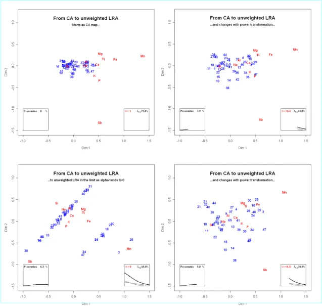
The glass cup data constitute a 47×9 compositional matrix, with the complication being that the component manganese (Mn) takes on only three small percentage values 0.01%, 0.02% and 0.03%, due to rounding of the percentages to two decimals. This engenders large ratios for this component, which causes it to dominate the solution in a two-dimensional map of unweighted log-ratios. In CA, apart from the different metric used, the components are weighted proportional to their marginal averages and the problem is essentially eliminated. Figure 1 shows, both statically and dynamically, the smooth change from CA to an unweighted LRA, i.e., using power family 1 defined in Section 1. In the static version we show four frames, in clockwise order: top left is the CA (with power parameter α =1), top right when α = 0.67, bottom right when α =0.33 and bottom left is the unweighted LRA in the limiting case as α→0. The dynamic version can be observed by clicking anywhere inside this figure – this gives a much clearer picture of the change, showing how Mn becomes more and more influential as we proceed towards the log-ratio transformation where each component is weighted equally. In the unweighted LRA we see diagonal bands of points corresponding to the subsamples with the three respective values of Mn – these are stretched out diagonally according to their values of another rare element, antimony (Sb), which also contributes highly to the unweighted LRA solution.

Figure 1: Transition from CA (top left) to unweighted LRA (bottom left), as the power parameter α changes from 1 to (in the limit) 0. The figures should be read clockwise. Clicking on this figure will

reveal the video of the whole transition.

Several additional diagnostics are shown in boxes in each of the above figures, and can be viewed changing dynamically in the video: at bottom left the Procrustes statistic between the original row configuration and the present one is given as a percentage of the total sum-of-squares; at bottom right the total inertia is shown in the upper solid curve and the first two eigenvalues below them. Note that we show the trajectories on the right as the power parameter drops, with the corresponding Procrustes curve moving to the right (i.e., the horizontal axis of the right box goes from α = 1 on the right to α→0 on the left, while the one on the left has the horizontal axis reversed). In this example we see that the inertia is increasing steeply with the power transformation. This large change of scale is taken into account by the Procrustes statistic, so the difference in the final row configuration is only 6.5% different from the first one. In the video you will notice a substantial rotation in the configuration around the value α=0.20, due to the two eigenvalues becoming almost equal (this can be seen in the righthand box) – at this value we have slowed the video down so that this rotation is more easily observed.

3 CA to weighted LRA

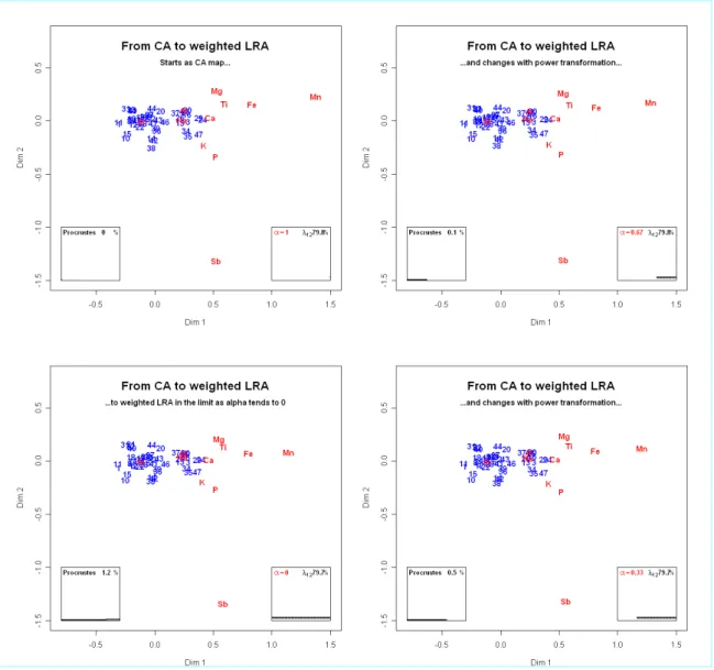
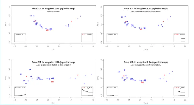
The next pair of analyses consists of CA and the weighted form of LRA, i.e., power family 2 defined in Section 1. Figure 2 and its accompanying video shows that the transition hardly changes the map – this illustrates the result that when the inertia is low, as in this example (total inertia = 0.00237), the results of CA and weighted LRA are very similar (see, for example, Greenacre and Lewi, 2005b). In the application of Section 6 the data have high inertia and there will be a bigger difference between the two analyses.

Figure 2: Transition from CA (top left) to weighted LRA (bottom left), i.e., spectral map, as the power parameter α changes from 1 to (in the limit) 0. The figures should be read clockwise and clicking on this

figure will reveal the video of the whole transition.

4 Unweighted to weighted LRA

To complete this study of the trilogy of methods, CA, weighted and unweighted LRA, we shos the transition between unweighted and weighted LRA. The two methods are linked not by a power

parameter but by the weights assigned to the columns (components) of the compositional data matrix. In the unweighted case these weights are 1/J, where J = 11 the number of columns, while in the weighted case the weights are cj, j=1,…,11, the column averages. Putting these weights in diagonal matrices, (1/J)I

and Dc respectively, we define a convex linear combination of the weights, as proposed by Greenacre

(2007):

Weighting scheme: D_w = β (1/J) I + (1 – β) Dc (2)

Thus, by letting the parameter β change smoothly from 1 to 0 and using the weights in D_w, all analyses between the unweighted case (β = 1) and the weighted case (β = 1) will be generated. Because the weighted LRA is very similar to the CA this generates a sequence which is almost exactly the reverse sequence observed in Figure 1, so we do not show it here, only in the oral presentation. But Table 1 shows numerically the contributions of the 11 components to the unweighted and weighted solutions in two dimensions: the contrinbution of Mn is considerably reduced in the weighted solution, which was the intention, while the contribution of the most common element silica (Si) has increased.

PCA 10.42 9.66 11.20 9.49 9.38 6.57 8.17 9.22 9.58 7.00 9.33

4 CA to PCA

The same idea can be used to compare CA with principal component analysis (PCA), where CA standardizes by the square root of the mean and PCA by the standard deviation. As before, the standardization is defined parametrically:

Standardization scheme: Dm = γ D_c–½ + (1–γ )D_s–1 (3)

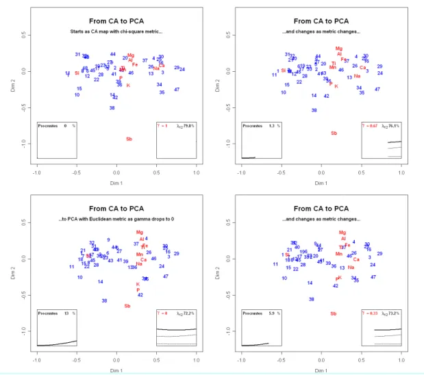
where the column standard deviations are in the diagonal of D_s. As γ varies from 1 to 0, the maps pass smoothly from CA (chi-square metric) to PCA (standardized Euclidean). Because the scales induced by the two metrics are very different, an adjustment is needed to keep the changing configurations comparable – we did this by multiplying the second term in (3) by the ratio of the square roots of the total inertias in the CA and the PCA. The CA solution is scaled as a standard CA biplot (Greenacre, 2007), which is directly comparable to the scaling of the PCA biplot. The results are shown in Figure 3.

Figure 3: Transition from CA (top left) to standardized PCA (bottom left). The figures should be read clockwise; clicking on this figure will reveal the video of the whole transition. The CA map is scaled as a

standard CA biplot, so the rare elements (e.g., Mn) are pulled towards the centre of the map. Also, the vertical inertia scale in the box at bottom right has been magnified compared to previous figures. Table 1: Contributions of components to

the two-dimensional solutions in the unweighted and weighted LRAs. In addition, the corresponding contributions are given for the two-dimensional standardized PCA (see Section 4) – these are more evenly spread out because variances are equalized in the PCA standardization.

unweighted weighted Si 7.11 21.05 Al 2.57 2.76 Fe 2.15 4.34 Mg 2.94 3.44 Ca 0.51 25.93 Na 2.89 22.33 K 0.23 2.20 Ti 1.92 0.53 P 0.80 0.37 Mn 39.48 0.37 Sb 39.39 16.68

5 Three-dimensional rotation

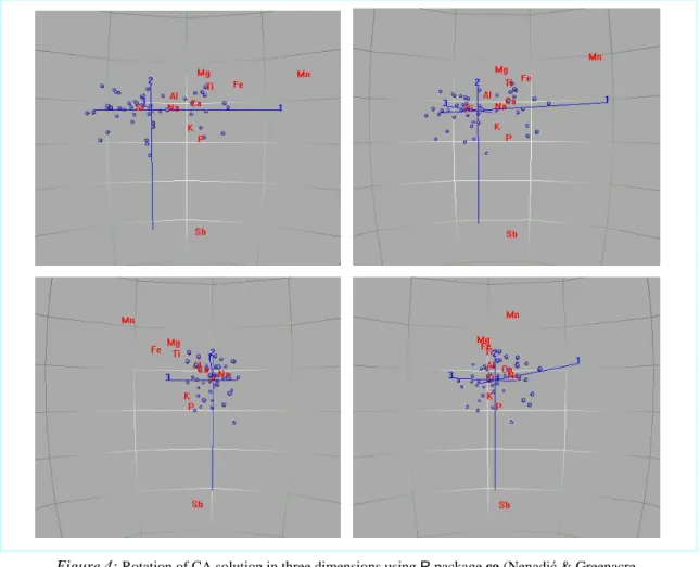
While we are demonstrating some videos, we include one of a rotation of the Baxter data in three dimensions. Figure 4 again shows four views, starting from the view with respect to dimensions 1 and 2 and ending with the view of dimensions 3 and 2, in other words rotating around the vertical dimension 2. The rotation shows that the component sodium (Na), which lies in the middle of the map in the initial two-dimensional projection, opposes all the other components along the third dimension (see final image at bottom left).

Figure 4: Rotation of CA solution in three dimensions using R package ca (Nenadić & Greenacre, 2007). The figures should be read clockwise and clicking on this figure will reveal the video of the whole

transition. The sample points, depicted by unlabelled balls, have been scaled up to improve their visualization.

6 CA and LRA on the population genetic data

To conclude our comparison of CA and LRA, we consider the MN population genetic data, a 24×3 matrix which is two-dimensional and which has high inertia (total inertia = 0.449). As shown by Greenacre and Lewi (2005b) there is a noticeable difference between the CA solution, which shows the populations along a curve, and the LRA solution, which shows the three genetic groups and the populations much more linear, and thus conforming to a equilibrium relationship. Figure 4 shows the transition, and in the video one can observe dynamically the straightening out of the configuration. There is very little

difference between the weighted and unweighted forms of LRA in this example because the three column means are not so different.

Figure 5: MN genetic data, showing transition from CA (top left) to weighted LRA (bottom left), i.e., spectral map, as the power parameter α changes from 1 to (in the limit) 0. The figures should be read

clockwise and clicking on this figure will reveal the video of the whole transition.

Acknowledgements

The support of the Fundación BBVA in this research is gratefully acknowledged as well as partial support by the Spanish Ministry of Education and Science, grant MEC-SEJ2006-14098.

References

Aitchison, J. (1980). Relative variation diagrams for describing patterns of variability in compositional data. Mathematical Geology 22, 487–512.

Aitchison, J. (1983). Principal component analysis of compositional data. Biometrika 70, 57–65. Aitchison, J. (1986). The Statistical Analysis of Compositional Data. London: Chapman & Hall. Aitchison, J. & Greenacre, M.J. (2002). Biplots of compositional data. Applied Statistics 51, 375–392. Baxter, M.J., Cool, H.E.M. and Heyworth, M.P. (1990). Principal component and correspondence

analysis of compositional data: some similarities. Journal of Applied Statistics 17, 229–235. Greenacre, M.J. (2007). Correspondence Analysis in Practice, Second Edition. London: Chapman &

Hall/CRC Press.

Greenacre, M. J. and Lewi, P. J. (2005a). Weighted logratio biplots, correspondence analysis and spectral maps. Paper presented at Compositional Data Analysis Workshop CODAWORK 2005, University of Girona.

Greenacre, M. J. and Lewi, P. J. (2005b). Distributional equivalence and subcompositional coherence in the analysis of contingency tables, ratio scale measurements and compositional data. Economics Working Paper 908, Universitat Pompeu Fabra. Accepted for publication in Journal of Classification. URL http://www.econ.upf.edu/en/research/onepaper.php?id=908

Greenacre, M.J. (2007). Power transformations in correspondence analysis. Economics Working Paper 1044, Universitat Pompeu Fabra. Accepted for publication in Computational Statistics and Data Analysis. URL : http://www.econ.upf.edu/en/research/onepaper.php?id=1044 Lewi, P.J. (1976). Spectral mapping, a technique for classifying biological activity profiles of chemical

compounds. Arzneim. Forsch. (Drug Res.) 26, 1295–1300.

Nenadić, O. and Greenacre, M. J. (2007). Correspondence analysis in R, with two- and three-dimensional graphics: The ca package. Journal of Statistical Software, 20 (1).