building water damage
Ola Haug Xeni K. Dimakos
Jofrid F. V˚ardal Magne Aldrin
Norwegian Computing Center P.O.Box 114, Blindern
N-0314 OSLO
E-mail address [email protected]
Abstract
The insurance industry, like other parts of the financial sector, is vulnerable to climate change. Life as well as non-life products are affected, and knowledge of future loss levels is valuable. Risk and premium calculations may be updated accordingly, and dedicated loss-preventive measures can be communicated to customers and regulators. We have established statistical claims models for the coherence be-tween externally inflicted water damage to private buildings and se-lected meteorological variables. Based on such models and downscaled climate predictions from the Hadley centre HadAM3H climate model, the estimated loss level of a future scenario period (2071-2100) is com-pared to that of a recent control period (1961-1990). On a national scale, payments increase by 15% and 20% under two different CO2
emissions scenarios, but there is substantial regional variability. Of the uncertainties inherently involved in such predictions, only the er-ror due to model fit is quantifiable.
Key words: Water damage, buildings, meteorological observations, climate model data, Generalized Linear Models, claims models, prediction.
1
Introduction
Over the past few years climate change has fully been put on the agenda of various fields of the society. In particular, since IPCC released their 4th annual report on climate change and its consequences last year, discussions have become more acute. One major aspect of the public debate is whether effort should be put into force on the current indication of climate change or if one should rather wait and see due to the considerable uncertainty that encloses this area.
As part of the financial sector, the insurance industry faces substantial chal-lenges from possible climate change. This applies to life as well as non-life insurance. Non-life insurance companies like Gjensidige Forsikring situated in Norway are concerned about assets held by their customers. With such duties, they share a genuine interest in climate change and its impact on future loss levels. Based on improved insight into future threats, insurance companies may update their risk and premium calculations, and announce dedicated preventive measures to customers, building contractors and regu-lators.
This paper reports on a study of water damage to private buildings. Based on daily claims data and contemporary historical weather data, claims mod-els for the coherence between losses and relevant weather variables are de-rived. Combined with climate scenario data, these models provide estimates of future loss levels.
We acknowledge Gjensidige Forsikring for their kind co-operation and for access to their claims database.
2
Data
The data used in this study are insurance data and meteorological and hydrological data from each Norwegian mainland municipality, a total of 431 sets of multivariate time series.
2.1 Insurance data
Insurance claims and population data are available from Gjensidige For-sikring’s own portfolio on private buildings for the period 1997-01-01 to 2006-12-31 (illustrated via the solid blue line of Figure 3). For a certain municipality, claims data constitute daily figures on the number of water claims and their corresponding total payment (index-linked). Population data are monthly and hold information on the number of policies.
The claims data are frequency claims,i.e. rather small losses that occur “of-ten”. They comprise externally inflicted water damage rising primarily from either precipitation, surface water, melting of snow, undermined drainage or blocked pipes.
Damage to buildings due to major catastrophes like flood, storm, slide etc. are covered mainly through the Norwegian Natural Perils Pool (see http://www.naturskade.no). Such losses are not part of our analysis. The Perils Pool is a compulsory regulation that mutually divides responsibilities among insurance companies operating in Norway.
Claim frequencies and mean claim size over the model period 1997 – 2006 are illustrated for selected municipalities through the thematic maps in Figure 1.
Figure 1: Claim frequency (number of claims per 100 policies, left) and mean claim size (total payment divided by the total number of claims, right) for the model period 1997 – 2006. Numbers are for each municipality.
2.2 Meteorological and hydrological data
Meteorological and hydrological data are naturally categorized into obser-vation based data and climate model data. The former exists for the time period from 1961-01-01 to 2006-12-31, and the latter for a control period and scenario period, ranging from 1961-01-01 to 1990-12-31 and from 2071-01-01 to 2100-12-31, respectively. In Figure 3, the meteorological observations are shown in red, whereas the climate model data constitute solid green lines. Data from both categories are daily values of precipitation, temperature, runoff and snow water equivalent. The variables have been spatially inter-polated and exist at municipality level. The interpolations are based on the most densely populated areas of a municipality only. Since these are the ar-eas where losses will primarily occur, a desirable coherence between claims and weather data is obtained.
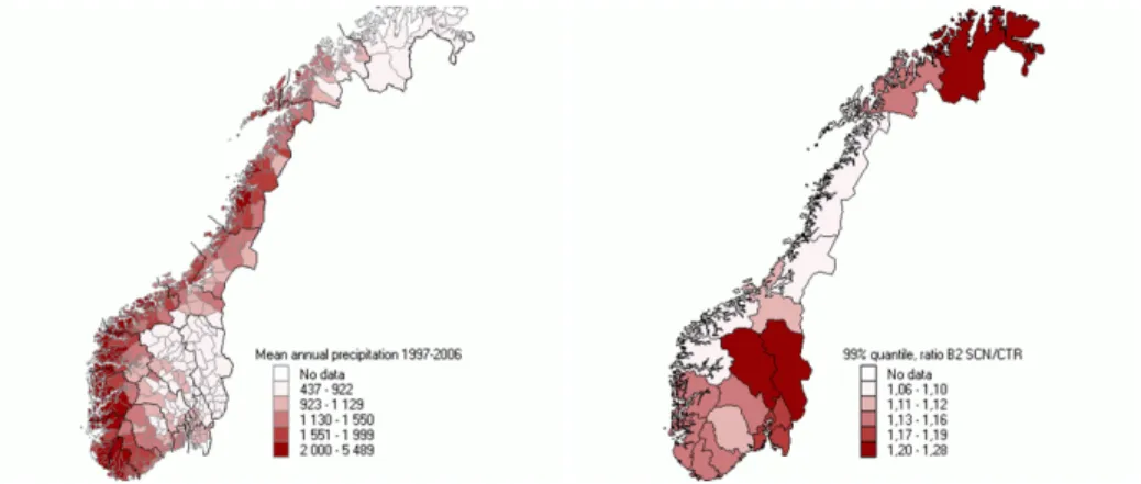
The large geographical variation in mean annual precipitation is illustrated through the thematic map to the left in Figure 2. The right panel of the fig-ure reveals countywise change in daily extreme precipitation to be expected from the control to the scenario period under the B2 emissions scenario. The change is expressed as the ratio of the empirical 99% quantiles of the set of all daily precipitation data for the two periods.
Figure 2: Left: Mean annual precipitation (in mm) over the model pe-riod 1997 – 2006. Numbers are for each municipality. Right: Change in precipitation from the control period to the scenario period under the B2 emissions scenario expressed as the ratio of 99% quantiles. Numbers are for each county.
The climate data are regionally downscaled and locally adjusted Hadley Institute HadAM3H global model runs under the CO2 emissions scenarios
A2 and B2. The scenario A2, which is the more CO2-intensive of the two,
prescribes high population growth rate and rapid economic development, whereas B2 relies on environmental conservation and sustainable growth, economically as well as socially.
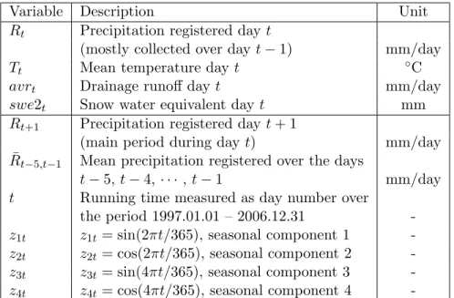
Table 1 summarizes the weather observations and the HadAM3H model data variables (above the horizontal line). Also listed are further variables used for modelling the claims. These include weather related as well as non-weather related variables.
Variable Description Unit
Rt Precipitation registered dayt
(mostly collected over day t−1) mm/day
Tt Mean temperature day t ◦C
avrt Drainage runoff day t mm/day
swe2t Snow water equivalent day t mm
Rt+1 Precipitation registered dayt+ 1
(main period during dayt) mm/day
¯
Rt−5,t−1 Mean precipitation registered over the days
t−5, t−4,· · ·, t−1 mm/day
t Running time measured as day number over
the period 1997.01.01 – 2006.12.31
-z1t z1t= sin(2πt/365), seasonal component 1
-z2t z2t= cos(2πt/365), seasonal component 2
-z3t z3t= sin(4πt/365), seasonal component 3
-z4t z4t= cos(4πt/365), seasonal component 4
-Table 1: Weather variables directly available from observation data and climate model data (above the horizontal line). Further variables used for claims modelling are listed below the horizontal line.
Rt+1, the dayt+ 1 precipitation, is included since the measurement period
for precipitation is 6 hours delayed compared with calendar time. That is, precipitation registered dayt+ 1 is the amount collected from 06 UTC day
¯
Rt−5,t−1 expresses accumulated precipitation and is meant to account for
water saturation of ground and vegetation. This is possibly relevant for the claims level on dayt.
The trend term,t, and the seasonal variables,z1t, . . . , z4t, take care of effects for which we do not know explicit explanatory variables. For instance, for the trend term one such factor that is not linked to weather could be economic activity.
3
Analysis
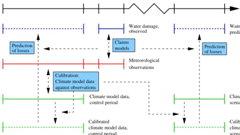
Figure 3 shows a flowchart that links the data referred in Section 2 to certain processing modules (blue boxes). Solid lines indicate original insurance or weather data, whereas processed data are drawn using dashed lines.
Water damage, observed 1990 1997 time 1961 Water damage, predicted observations models 2006 Calibration: Climate model data against observations
control period scenario period Climate model data, Climate model data,
Calibrated climate model data, control period
climate model data, Calibrated scenario period Control period Meteorological Prediction of losses of losses Prediction Prediction period Claims
3.1 Claims models
Statistical models that relate losses to weather conditions are worked out separately for the number of claims and for the claim severity. Both re-sponses are modelled using Generalized Linear Models (GLM)(seee.g. Mc-Cullagh and Nelder (1989)), i.e. models of the form
g(µ) =g(E(Y)) =β0+
p
X
i=1
βixi. (1)
Here, Y is the response with µ = E(Y), g(·) is the link function and
x1, . . . , xp are explanatory variables including the weather elements. The model coefficients β1, . . . , βp are determined from the data through the model fit.
The number of claims on day t, Nt, is modelled through a quasibinomial model,
Nt∼quasiB(At, pt)
E(Nt) =Atpt (2)
Var(Nt) =φ Atpt(1−pt).
Here,Atis the number of policies andptthe claims probability on dayt. In-clusion of the dispersion parameterφdestroys the pure likelihood properties of the binomial model, but at the same time allows for increased variability as seen in the claims data.
Daily claims data are fit through a logistic regression in the GLM (1), i.e. logitpt= log pt 1−pt =β0+ p X i=1 βixit. (3)
The use of a (quasi-)binomial distribution forNtensures that the number of claims does not exceed the number of policies at a certain day. An alternative would be the more common Poisson model. This model, however, does not impose an upper limit on the number of claims, an attribute which is crucial when we later turn to prediction. The models are related, though,
the Poisson model being a limiting model for the binomial model for At large and pt small (Feller (1968)).
Next, turning to claim severity, we letstj denote the size of the j’th claim on dayt,j= 1, . . . , Nt. We assume thatstj follows a Gamma distribution,
stj∼Gamma(ξt, ν), (4)
with parameters so that E(stj) = ξt and Var(stj) = ξt2/ν (McCullagh and Nelder (1989)). In our models, claim severity is measured by the daily mean claim size, St= Nt X j=1 stj/Nt. (5)
The assumption (4) implies that for a given number of claims, the average claim size on daytobeys
St|Nt∼Gamma(ξt, νNt)
E(St|Nt) =ξt (6)
Var(St|Nt) =ξt2/(νNt).
We apply a logarithmic link function to the expectationξtin the GLM and let logξt=α0+ p X i=1 αixit (7)
for explanatory variables xit, i = 1, . . . , p. In the process of fitting the model (7), the number of claims is used as a weight so that mean claim severities based on several claims count for more than claim size averages based on fewer claims.
Once models are established for the number of claims and their mean size, the expected total payment on day tis expressed through
E( Nt X j=1 stj) = E(NtSt) = E(Nt)E(St|Nt) (8) =Atptξt.
3.2 Model fitting
Prior to GLM model fitting, reasonable parametric forms for the explana-tory variables are spotted from fitting Generalized Additive Models (GAMs) (see Hastie and Tibshirani (1990)). In such a framework the coefficient terms
βixi in equation (1) are replaced by smooth functionsfi(xi) of the explana-tory variables. From subjective inspection of GAM plots, a selection of the most appropriate function alternatives are combined into candidate GLMs. Gjensidige Forsikring wants high-resolution claims models in order to iden-tify vulnerability at municipality level. However, compared to the exposure, losses are rare and fitting separate claims models for each municipality is infeasible. Rather, claims models are fit on unified data sets that involve larger spatial areas (data records are still at municipality level).
For the number of claims, models are fitted countywise. We keep some spatial structure in that the β0 constant term of (3) is split into a mean
county level term ˜β0 and a correction term δk for every municipality k in the current county. δkis positive- or negative-valued and satisfiesPkδk = 0. The remaining coefficientsβi are common to all municipalities in the same county.
Claim severity data are more sparse as days with zero claims are uninforma-tive. In order to obtain reasonable model fits, the spatial entity has to be enlarged beyond counties as are used for the number of claims. Gjensidige Forsikring divides Norway into five geographical regions, each comprising from two up to five counties. Similar to what is done for the number of claims models, claim severity models are fit separately to those regions. The constantα0 of Equation (7) is split into a region component ˜α0 and an
adjustment termγF(k)that is identical for each municipalitykinside county
F(k) in the current region.
Model selction is made by means of the Bayesian Information Criterion (BIC) originally described by Schwarz (1978). We sum BIC measures over all the spatial entities for which the models are fitted (i.e. counties for the number of claims, and regions for the claim size). The final models forpkt
and ξktare given by logitpkt= ˜β0+δk
+β1z1t+β2z2t+β3z3t+β4z4t
+β5t+β6t2+β7t3 (9)
+β8Rk(t+1)+β9Rkt
+β10Tkt+β11Tkt2 +β12log(avrkt) +β13swe2kt and logξkt= ˜α0+γF(k) +α1z1t+α2z2t+α3z3t+α4z4t +α5t+α6t2+α7t3 (10) +α8Rk(t+1)+α9Rkt+α10avrkt, respectively.
Essentially, the BIC criterion suggests leaving out variables that do not explain sufficiently the response of the model. For instance, precipitation typically has a positive effect (significant and with little uncertainty) on the claim level, while the effect for other weather variables is often more unclear. However, even if a variable has a non-significant effect, one can not deduce it is not important. The lack of effect is most likely due to considerable estimation uncertainty rather than the effect being zero with tiny confidence bands.
3.3 Prediction
Expected losses for specific weather conditions may be predicted from the claims models (9) and (10) by inserting corresponding values for the me-teorological variables. Consequently, using future climate data from the HadAM3H model described in Section 2.2, future loss expectations may be quantified, see Figure 3. The same exercise may be performed on climate model data from the control period. Finally, the expected loss levels of the two periods may be compared and possible shifts identified.
Predictions of future insurance losses is for sure associated with uncertainty. First, of course, there is the uncertainty inherent in the climate model data
at hand. This error is not stated, but there are studies that suggest that it can be considerable, in particular at local scales (see e.g. Stainforth et al. (2007)). Second, there is an error present due to model specification. Our claims models certainly deviate from the true model for the phenomenon under study. Leaving out non-significant variables as discussed above is part of this error. However, as the true model is unknown, this error is left unattended. A third source of error is introduced from fitting the selected claims models. The coefficients are estimated up to some precision as told by the data. This estimation uncertainty is the only uncertainty that can be quantified. In view of these aspects, our results should be interpreted as guidelines of whatcould happen in the future, with rough margins in either direction.
Loss level predictions for the scenario period are compared with predictions made from climate model data in the control period. For every day in each of the periods, predictions for the number of claims (Nbt), the mean claim
size (Sb¯t) and the total payment (Ubt) are derived from Equations (2), (6)
and (8), giving b Nt = Atpbt, (11) b¯ St = ξbt, (12) b Ut = Atpbtξbt. (13)
Rather than focussing loss levels as such, we consider thechange from the control to the scenario period stated as ratios. For instance, for the number of claims in municipalityk, we fix the number of policies (=A0) and consider
rk(scn, ctr) = P t∈scnpb scn kt |Akt=A0 P t∈ctrpb ctr kt|Akt=A0 . (14)
Here, “scn” and “ctr” signify the scenario period and the control period, respectively. Since both periods consist of 30 years, the nominator and the denominator are of comparable size.
Similarly, for the mean claim size we consider the total payment divided by the total number of claims throughout each of the periods. The ratio of the scenario to the control period reads
rk(scn, ctr) = (P t∈scnξbtscn·pbscnt )/( P t∈scnpb scn t ) (P t∈ctrξbtctr·pbctrt )/( P t∈ctrpb ctr t ) . (15)
And for the expected total payment the ratio is simply the ratio of the sum of payments throughout each of the periods,
rk(scn, ctr) = P t∈scnpb scn t ·ξbtscn P t∈ctrpb ctr t ·ξbtctr . (16)
Ratios larger than one indicate an increased loss level in the future scenario period. County level figures are achieved from weighting the ratios in Equa-tions (14), (15) and (16) by the number of policies in each municipality at the last day of the model fitting period.
The climate model data we have used for prediction are massive and de-tailed output from a numerical model. They have not undergone any mete-orological quality control. Some of these data contain spurious spikes that are probably not connected to climate change, but rather a consequence of numerical instabilities. In order to minimize the effect of such outliers, pre-dicted loss levels have been truncated at their empirical 99.5% quantile. This is applied to the variable sets produced from Equations (11), (12) and (13) for both the control and scenario periods, before calculating ratios (14), (15) and (16).
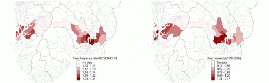
Point estimates of the predicted ratios in Equation (14) for the B2 emissions scenario are illustrated for some municipalities in the left panel of Figure 4. For reference, claim frequencies for the model period 1997 – 2006 for the same municipalities are also included (right panel). The outcome for each municipality will be a funtion of the local vulnerability as told by the claims model, as well as the future climate as predicted by the emissions scenario under study. As is evident from the maps in Figure 4, among the munic-ipalities with the lowest claim frequencies during the model period, there are municipalities whose claim frequency will stay low also in the future. In an opposite position are municipalities which have experienced high claim frequencies historically, and are still to expect a sizeable increase also in the future. In between, there are municipalities with low claim frequencies dur-ing the model period, that will gain noticeably more claims in the future. And also, we find municipalities that have faced high claim frequencies in the past, but will hardly have to fear any further growth.
Figure 5 displays the change in number of claims from the control to the sce-nario period at county level as given by a weighted version of Equation (14). Only counties that contain the municipalities depicted in Figure 4 are given.
Figure 4: Left: Prediction point estimates of the change in number of claims from the control period to the scenario period under the B2 emissions sce-nario. Right: Claim frequency (number of claims per 100 policies) for the model period 1997 – 2006. Numbers are for each municipality.
Uncertainty intervals account for estimation uncertainty only and have been derived from assuming a multinormal distribution for the model coefficients. The intervals are formed from the 10% and 90% empirical quantiles of 100 model simulations. ● ● ● ● Ratio Norway Hordaland Buskerud Akershus 0.9 1.0 1.1 1.2 1.3 1.4 ● ● A2/ctr B2/ctr ● ● ● ●
Figure 5: Prediction of the change in the number of claims from the control to the scenario period. Point estimates and approximate 80% confidence intervals. A2/ctr signifies ratios for the A2 CO2 emissions scenario, while
4
Conclusions
In this study we have established claims models that quantify the statisti-cal coherence between water building damage and different aspects of the weather. The analysis is restricted to private houses, and losses due to extreme events like flood, storm surge or landslide are not included. The weather has been described through the variables precipitation, tempera-ture, runoff and snow water equivalent.
The claims models have been combined with climate model data for a his-toric control period and a future scenario period to infer hishis-toric and future loss levels. Results for two different CO2 emissions scenarios have been
worked out, and changes from the control period to the scenario period are presented as ratios.
Our analysis shows that losses will increase under both emissions scenarios. Nationwide, the expected total payment increases by 20% and 15% under the scenarios B2 and A2, respectively. There is considerable geographic vari-ability, however, as exemplified through a countywise range from 11% to 44% in the payments under the B2 emissions scenario. In general, coastal regions in the south-eastern part of Norway are more vulnerable than are counties in the western and middle parts of the country. Additional to estimation uncertainty, there is considerable unquantifiable uncertainty transferred to the loss predictions both from the climate model data and the model speci-fication.
It should be pointed out that the above figures are subject to a building mass as of the end of the model fitting period, both with respect to architectural tradition and location of the houses. The increasing focus on climate change is supposed to influence building practice, however, and thereby contribute in the direction of limiting the loss level enlargement. The relatively long period between the control and the scenario periods makes such adaptations possible. One should remember, though, that measures taken to reduce risks still induce costs, the major advantage compared to not adapting at all perhaps being the inconvenience of damages thus avoided by the policy holders.
References
Feller, W. (1968). An introduction to Probability Theory and Its Applica-tions, volume 1. New York: John Wiley, 3 edition.
Hastie, T. J. and Tibshirani, R. J. (1990). Generalized additive models. Chapman & Hall.
McCullagh, P. and Nelder, J. A. (1989). Generalized Linear Models. Chap-man & Hall, second edition.
Schwarz, G. (1978). Estimating the dimension of a model. Annals of Statis-tics, 6(2):461–464.
Stainforth, D. A., Allen, M. R., Tredger, E. R., and Smith, L. A. (2007). Confidence, uncertainty and decision-support relevance in climate predic-tions. Phil. Trans. R. Soc. A, 365:2145–2161.