WORKING PAPER 2002:21
Optimal unemployment
insurance with monitoring
and sanctions
Jan Boone
Peter Fredriksson
Bertil Holmlund
Jan van Ours
WP 2002-21.qxd 02-12-10 08.04 Sida 1Optimal unemployment insurance with
monitoring and sanctions
∗
Jan Boone† Peter Fredriksson‡ Bertil Holmlund§ Jan van Ours¶ 26 November 2002
Abstract
This paper analyzes the design of optimal unemployment insurance in a search equilibrium framework where search effort among the un-employed is not perfectly observable. We examine to what extent the optimal policy involves monitoring of search effort and benefit sanc-tions if observed search is deemed insufficient. We find that intro-ducing monitoring and sanctions represents a welfare improvement for reasonable estimates of monitoring costs; this conclusion holds both relative to a system featuring indefinite payments of benefits and a system with a time limit on unemployment benefit receipt.
JEL-classification: J64, J65, J68
Keywords: Unemployment insurance, search, sanctions
∗We gratefully acknowledge comments from Anders Forslund, David Grubb, Åsa
Rosén and seminar participants at IZA, Bonn, Stockholm University, University of Copenhagen, University of Gothenburg, and University of Cyprus. Financial support from the Swedish Council for Working Life and Social Research (FAS) is gratefully acknowledged.
†Department of Economics and CentER for Economic Research, Tilburg University,
OSA and CEPR. Postal address: Box 90153, 5000 LE Tilburg, The Netherlands. E-mail: j.boone@uvt.nl
‡Department of Economics, Uppsala University, IFAU and CESifo. Postal address:
Box 513, SE-751 20 Uppsala, Sweden. E-mail: peter.fredriksson@nek.uu.se
§Department of Economics, Uppsala University and CESifo. Postal address: Box
513, SE-751 20 Uppsala, Sweden. E-mail: bertil.holmlund@nek.uu.se
¶CentER for Economic Research, Tilburg University, OSA, IZA and CEPR. Postal
1
Introduction
It is generally accepted that public provision of unemployment insurance (UI) is socially desirable in a world with risk averse individuals. However, it is also well established that the provision of UI does not come without adverse incentive effects. For example, more generous UI benefits is likely to reduce search effort and raise wage pressure, thus causing some increase in unemployment. The problem facing policy makers is thus to strike an optimal balance between the insurance benefits on the one hand, and the adverse incentive effects on the other hand. This problem has been the subject of several recent papers. Our paper contributes to this literature by recognizing that the government may condition benefit payments on (imperfectly) observed search effort. This leads us to an analysis of optimal UI design in a search equilibrium framework where the government has several policy instruments at its disposal, including the benefit level, the rate at which search effort is monitored, and the magnitude of the sanction in case search effort is regarded as insufficient. We find that a system with monitoring and sanctions represents a welfare improvement relative to other alternatives for reasonable estimates of the monitoring costs.
Our results on the desirability of monitoring can be contrasted with a well-known result that dates back to Becker’s (1968) celebrated paper on optimal crime deterrence. In Becker’s analysis (as in ours), monitoring is costly because resources have to be spent on detecting crime (violations of search requirements). Punishment, in the form of a fine (sanction), goes without cost since it involves a transfer of money from one individual to others. To deter crime the expected fine, i.e., the probability of being caught times thefine, should be big enough. By raising thefine, monitor-ing costs can be reduced without affectmonitor-ing incentives for crime. However, Becker’s analysis presupposes risk neutral agents. When agents are risk averse and there are errors in the monitoring technology, Becker’s result need not hold. If the monitoring technology is plagued by Type II errors, some complying individuals are sanctioned and these individuals will be subjected to substantial welfare losses when fines are high.1
1This squares with the conclusion in Polinsky and Shavell (1979). They conclude
that risk aversion weakens the case for the Beckerian policy prescription. Furthermore, they note that the possibility of making Type II errors reinforces this conclusion. See Garoupa (1997) and Polinsky and Shavell (2000) for recent surveys of the economic theory of law enforcement.
Shavell and Weiss (1979) presented a seminal analysis of optimal se-quencing of benefit payments over the spell of unemployment. The key result was that the benefit level should decline monotonically over the unemployment spell, because such a profile involves stronger incentives to search. Recently a number of papers have extended the analysis of Shavell and Weiss. One strand of the literature adds additional policy instruments; Hopenhayn and Nicolini (1997) is a case in point. Another strand of the literature (e.g. Cahuc and Lehmann, 2000, and Fredriksson and Holmlund, 2001) takes account offirm behavior and allows for endogenous wage de-termination. Endogenous wages is potentially important since a declining benefit profile can raise wage pressure. Wage pressure may rise because it is the value of unemployment upon unemployment entry that enters the worker’s outside option. The analysis in Fredriksson and Holmlund (2001), however, suggests that there is still a case for having a declining profile of benefit payments.
The contributions reviewed above, and most of the other literature on optimal UI, do not consider that the government can make the re-ceipt of benefits dependent on the unemployed worker’s search effort. As documented by Grubb (2001), existing UI systems condition benefit pay-ments on performance criteria such as “availability for work” and “active job search”. These criteria are enforced by some degree of monitoring of the benefit claimants. The requirements for job search show substantial variations across countries.
Failure to meet search requirements may result in a benefit sanction, i.e., a temporary or permanent cut in benefits. A typical duration of sanctions for afirst refusal of a suitable job offer is two to three months. Observed sanction rates — the total number of sanctions over a year relative to the stock of beneficiaries — also vary substantially across countries. For example, sanctions due to insufficient search hovered around 30 percent in the United States in the late 1990s, whereas other countries (Germany, Denmark, Norway) appear to have undertaken no sanctions related to search inactivity; see Grubb (2001) for further details.
Recent empirical work has shed light on the effects of changes in search requirements and monitoring of job search. The arguably most convincing evidence is based on randomized experiments undertaken in the United States. The “treatments” in these experiments involved the number of employer contacts, the required documentation and the frequency of
veri-fication.2 These studies indicate that either more intensive monitoring or more demanding search requirements tend to reduce the length of
bene-fit claims. Recent non-experimental evidence from the Netherlands and Switzwerland also suggest that the imposition of sanctions substantially raises the transition rate to employment (Abbring et al., 1997; van den Berg et al., 1998; Lalive et al., 2002). Our reading of the bulk of the evidence is that more intensive monitoring and more stringent search re-quirements do matter for search activity and transitions out of unemploy-ment.3
The literature on monitoring and sanctions in the context of UI is very small. The study most closely related to what we do in the present paper is Boone and van Ours (2000). The model is a version of the Pissarides (1990) search and matching model and has similarities with the model in Fredriksson and Holmlund (2001). A key feature of the model is that the unemployed and insured worker can affect the probability of continued UI receipt by the choice of search effort; the higher the search effort, the lower the risk of being exposed to a benefit sanction.
The analysis of monitoring and sanctions is clearly related to the analy-sis of the optimal sequencing of UI benefits. Indeed, one can think of the declining profile of benefit payments as an indirect “sanction” on defi -cient job search. The defining characteristic of a monitoring and sanction system, however, is that the risk of being sanctioned depends directly on search activity. This feature can have substantial implications for policy prescriptions. Let us illustrate this point by considering a world with risk aversion and a finite arrival rate of job offers. In this situation, a system with a time limit on UI benefit receipt can never have “Beckerian proper-ties”. The reason is that some workers will be penalized as time passes. However, a Becker-type solution is a distinct possibility when the risk of being penalized depends directly on search. If the monitoring technology is perfect, the government can implement the optimal search intensity by threatening to impose the maximal sanction.4
2
See OECD (2001), Johnson and Klepinger (1994), Benus et al. (1997) and Black et al. (1999).
3
There is at least one study, van den Berg and van der Klaauw (2001), that fails to confirm that more intensive monitoring affects transitions out of unemployment. The authors conjecture that the result may reflect that more stringent monitoring of formal search induces a substitution away from informal search channels.
4This a viable strategy with risk aversion since there will be no sanctions in
In this paper we extend the contributions by Boone and van Ours (2000) and Fredriksson and Holmlund (2001) by offering a normative analysis of a benefit system with costly monitoring and sanctions. The basic model features two benefit levels which can be thought of as unem-ployment insurance (UI) and unemunem-ployment assistance (UA), respectively. Workers who receive UI are monitored at a certain rate and, with some probability, exposed to a benefit sanction. The probability of being sanc-tioned depends on the worker’s search effort and the precision at which search effort can be observed by the UI provider. Sanctioned workers re-ceive UA, they are not monitored, and they need to become reemployed before they are entitled to UI. We are concerned with the characteristics of the optimal benefit system when there are four available policy instru-ments: the level of benefits in UI and UA (the difference between the two representing the sanction), the rate at which the unemployed worker en-titled to UI is monitored, and the precision of the monitoring technology that determines how the agent’s search effort affect the probability of a sanction.
The next section of the paper presents the basic model. Section 3 derives some analytical results concerning the properties of the optimal benefit system. In section 4, we turn to a numerical analysis of the optimal benefit system. Section 5 concludes.
2
The model
2.1
The labor market
We consider an economy with a fixed labor force, which is normalized to unity. Workers are either employed or unemployed and have infinite horizons. Time is continuous. An employed worker is separated from his job at an exogenous Poisson rate φ. Upon entering unemployment, the worker is immediately eligible for UI benefits.
Recipients of UI benefits are monitored with respect to their search behavior. If they fail to meet certain search requirements, they are exposed to a benefit withdrawal (a sanction). We assume that the sanction lasts for the remainder of the unemployment spell. At every instant, there are thus two groups of unemployed workers: eligible workers who receive benefits andsanctioned workers who have been exposed to a benefit withdrawal.
employ-ment for an eligible and asanctioned worker, respectively. The exit rates differ between the two groups to the extent that their search effort differ. Letsj,j=e, s, denote search effort. The effective number of searchers in the economy is then given as S =seue+ssus, where uj is the number of
unemployed in category j.
The matching function is of the usual constant returns to scale variety:
H = H(S, v), where v is the number of vacancies. Let θ ≡ v/S denote labor market tightness. The probability per unit time that individual i
escapes unemployment state j is then obtained as αji ≡ sjiH(S, v)/S = sjiα(θ). Also, α(θ) = H(S, v)/S = H(1, θ) and hence α0(θ) > 0; the tighter the labor market, the easier to find a job. Firms fill vacancies at the rateq(θ) =H(S, v)/v =H(1/θ,1), and thusq0(θ)<0; the tighter the labor market, the more difficult tofill a vacancy. By constant returns to scale, we also have α(θ) =θq(θ).
While unemployed and receiving UI benefits, an unemployed agent is monitored at rateµ. We think of monitoring as random inspections of the worker’s search activity. Given monitoring, there is some probability that the observed search effort does not meet the search requirement, in which case the worker is sanctioned. Let π(se) denote the probability of being sanctioned upon inspection of search effort, implying that UI recipients loose entitlement at the rate µπ(se).
Having defined the relevant transition rates, we can state the aggregate
flow equilibrium relationships of the labor market:
φn=αeue+αsus (1)
αsus =µπue (2)
wheren= 1−ue−usdenotes total employment in the economy. Thefirst equation pertains to employment whereas the second equation pertains to the state of unemployment with a sanction. Now we can use (1) and (2) to solve for employment:
n= λ(α
e+µπ)
φ+λ(αe+µπ) (3)
whereλ≡ue/(ue+us) =αs/(αs+µπ))is the ratio of eligible unemploy-ment to total unemployunemploy-ment.
2.2
Monitoring and sanctions
Let us make the monitoring and sanctions technology explicit. We choose a reduced form specification which allows us to have as special cases indef-inite payments of UI benefits (µ= 0),finite duration of UI benefit receipt
(µ > 0 and π(sei) = 1), and a monitoring and sanctions technology. In
particular, we assume that the probability of being sanctioned upon in-spection depends linearly on search: π(sei) = 1−σsei. Proposition 2 below gives conditions under which σ >0 is optimal. Further, we require that
π(se
i)≥0 for allsei ∈[0,1], which, in turn, implies thatσ∈[0,1].
The parameter σ measures to which extent the sanction probability depends on an agent’s own search effort. One way to interpretσ is that it indexes the precision of the inspection technology. For instance, σ = 0 corresponds to the situation where it is determined by lottery if the agent has searched to rule or not; therefore, everyone who is monitored is sanctioned irrespective of search intensity. Alternatively, σ = 0can be seen as a UI system with a time limit, as in Fredriksson and Holmlund (2001). If, on the other hand, σ is strictly positive the agent’s search effort matters for the sanction probability. The higher isσ, the higher the precision with which an agent’s search effort is observed and rewarded.5
Whereasσ = 0gives little direct incentive to search, it is an inexpensive system to operate. This is due to the fact that there are no inspections of agents’ search effort. On the other hand,σ >0gives a direct incentive to search but also implies that more monitoring officials are needed in order to inspect agents’ search intensities. So the monitoring cost per monitored agent is increasing inσ.
More precisely, we assume that the cost of running the monitoring and sanctioning system,C, is given by:
C=c(σ)µuew (4)
The costs of running the UI-system are increasing in the number of monitored individuals (µue). The rate of increase is determined byc(σ)≥
0. This cost depends on the precision of the inspection technology with
c0(σ) ≥0 and c(0) = 0. We think of the inspection of search as a labor
5
From a more general point of view, it is possible to derive this technology from “first principles” with the aid of a few assumptions. We present this derivation in Appendix A.
intensive activity and, therefore, the monitoring cost is proportional to the aggregate wage w.
2.3
Worker behavior
The employed worker’s (indirect) instantaneous utility is determined by his wage, w. The unemployed worker receives unemployment benefits,B, as long as he is eligible. When sanctioned, he receives Z. We show in proposition 1 below that B > Z. We assume that workers do not have access to a capital market, so consumption equals income at each instant. We take the utility functions to be strictly concave in income and leisure. The unemployed worker’s instantaneous utility is decreasing in search effort, since search reduces time available for leisure. The utility function for the eligible unemployed worker is υ(B, sei) and for the sanc-tioned worker it is υ(Z, ssi). The employed worker’s utility is given by
υ(wi, h), whereh denotes hours of work; we take h as exogenouslyfixed.
Letrdenote the subjective rate of time preference and letUj andEbe the expected present values of being unemployed,j=e, s, and employed, respectively. The value functions can then be written as:
rUie = max se i {υ(B, sei) +seiα(θ) (E−Uie)−µπ(sei) (Uie−Us)} (5) rUis = max ss i {υ(Z, ssi) +ssiα(θ)(E−Uis)} (6) rEi = υ(wi, h)−φ(Ei−Ue) (7)
The unemployed worker chooses search effort to maximize rUij. The
first-order conditions are given by:
υs(B, se) +α(θ)(E−Ue)−µπs(se) (Ue−Us) = 0 (8)
υs(Z, ss) +α(θ)(E−Us) = 0 (9)
where partial derivatives with respect to search effort are indicated by subscripts. In these expressions we have imposed symmetry, i.e., we have made use of the fact that workers are identical and choose the same search effort. Thefirst-order conditions convey the usual message:6 at the
opti-mum, the marginal cost of search should equal the marginal benefits. The
6The second-order conditions for a maximum are fulfilled by the concavity of υ(
·)
marginal cost is captured by foregone leisure, i.e.,υs(B, se) andυs(Z, ss).
The marginal benefit involves the gain in utility associated with a transi-tion to employment, i.e., α(θ)(E−Uj), j=e, s. For the eligible worker, there is an additional benefit of more intensive search, as revealed by the third term on the right-hand side of (8). More intensive search reduces the probability of being sanctioned, thus prolonging the expected duration of benefit payments. This does not imply, however, that eligible workers nec-essarily search harder than sanctioned workers. The effect pulling in the opposite direction is B > Z: sanctioned workers gain more fromfinding a job than eligible workers since E−Us > E−Ue holds in equilibrium. Which effect dominates depends on the parameters of the UI system.
We assume that the instantaneous utility functions take the form:
υ(m, l) = lnm+Γ(l), m={w, B, Z}, l={1−¯h,1−se,1−ss}
wheremdenotes (real) income, which depends on the worker’s labor mar-ket position. The employed worker receives a wagew; the eligible unem-ployed worker receives unemployment insurance, B; and an unemployed worker who has been exposed to a sanction receives unemployment assis-tance,Z. Furthermore, Γ(l) represents the value of leisure withΓ0(l)>0
andΓ00(l)<0.
2.4
Firms and wage bargaining
Assume that government expenditure on benefits and monitoring is fi -nanced by a proportional payroll tax paid byfirms. Labor productivity is constant and denotedy. The cost of holding a vacancy isky, withk >0. LetV denote the present value of a vacant job andJ the present value of an occupied job. The value functions are of the usual form:
rV =−ky+q(θ)(J−V) (10)
rJ =y−w(1 +t)−φ(J −V) (11)
where t is the proportional payroll tax rate. With free entry of new va-cancies,V = 0, we obtain the wage cost as proportional to the marginal product of labor, i.e.,
Definingwc≡w(1 +t) and writing the right-hand side of this equation as
d(θ)y,we refer towc=d(θ)y as the zero profit condition, withd0(θ)<0.
The outcome of the Nash bargain
max
wi
[E(wi)−Ue]β[J(wi)−V]1−β, β ∈(0,1)
is a relationship of the form:
E−Ue wυw = β 1−β J wc (13) whereV = 0and symmetry have been imposed. The Nash bargain implies a wage-setting relationship, i.e., a relationship between bargained wages and labor market tightness. We assume that the government fixes the replacement rates in this economy. Hence Z = zw and B = bw where
z and b are policy parameters. The replacement rates are defined with respect to the economy-wide average wage which the individual employee perceives to be independent of his wage demands; therefore ∂Ue/∂w= 0. Finally, the relative size of the benefit sanction is denoted by p, i.e. p
satisfies z= (1−p)b.
2.5
Equilibrium
Our assumptions imply that the model has a convenient recursive ture; the model in Fredriksson and Holmlund (2001) has a similar struc-ture. The zero-profit condition and the wage-setting relationship deter-mineθandwc. To see this, note that with free entry of vacancies we have
J = ky/q(θ) and wc = d(θ)y, which implies that the right-hand side of
(13) is increasing inθbut independent ofsj. Moreover, the left-hand side of (13) is a function of θ but independent of w given our chosen utility function and the fact that income during unemployment is proportional to the aggregate wage. It can also be shown that E−Ue is independent
of sj, an envelope property implied by optimal search behavior. With θ
determined, we get sj from (8) and (9), since the differences in present values are independent ofw. With θandsj determined, we obtainuj and
n from (1)-(3).
Notice thatθ,wc,sj,uj andnare independent of the tax rate,t. The
latter can be determined residually from the government’s budget restric-tion, noting that the government uses the wage tax tofinance benefits and monitoring costs:
twn=uebw+uszw+c(σ)µuew (14) With the tax rate determined, the worker’s take-home wage is obtained fromw=wc/(1 +t).
3
Optimal unemployment insurance
The optimal unemployment insurance system involves four instruments:
b,p,µ, andσ. We use a utilitarian welfare function, i.e., welfare (W)is
de-fined as: W =uerUe+usrUs+n(rE+rJ) +vrV whereV = 0by the free entry condition. We ignore discounting; hence it is valid to compare alter-native steady states without considering the adjustment process. With no discounting, the welfare objective simplifies to an employment-weighted average of instantaneous utilities, i.e.
W =nυ(w, h) +ueυ(B, se) +usυ(Z, ss) (15)
The optimal policy maximizes (15) subject to the market equilibrium conditions, sj =sj(b, p, µ, σ) andθ=θ(b, p, µ, σ), as well as the balanced budget constraint, t =t(b, p, µ, σ). Let ρ={b, p, µ, σ} denote the vector of policy parameters. Hence the vector of first-order conditions is given
by(dW/dρ) = 0.
Before proceeding to the numerical results it is useful to state two analytical results. First of all, the key result in Fredriksson and Holmlund (2001) applies directly. The following proposition reiterates proposition 2 in Fredriksson and Holmlund (2001)
Proposition 1 The optimal policy involves p >0, provided that an inte-rior solution todW/db= 0 exists.
Proof. The proof is by contradiction. Supposeb >0and consider the trial solutionp= 0.Atp= 0,thefirst-order condition forσ has a solution atσ = 0becausec0(σ)≥0. Moreover, the condition forµis irrelevant. So, let usfixµat some arbitrary, but interior, value: µ0 ∈(0,∞).The uniform benefit structure (p= 0) cannot be optimal if(dW/dp)>0atp= 0.Some manipulations of thefirst-order condition forp using dW/db= 0yields
µ dW dp ¶ p=0 = ∂W ∂ss ∂ss ∂p >0 (16)
where ∂W/∂ss >0 denotes the partial derivative of welfare with respect
to ss holding θ constant, and ∂ss/∂p > 0 is, again, defined holding θ
constant.
There are two key mechanisms that yield the sign of (16): there is a taxation externality associated with search and there is an “entitlement effect”. The taxation externality derives from the fact that, given that some insurance is optimal (b > 0), taxes are required to finance unem-ployment expenditure. Individuals, however, do not take into account that taxes can be lowered if search intensity (and hence employment) in-creases. Therefore,∂W/∂ss>0.Moreover, the so called entitlement effect (c.f. Mortensen, 1977) will operate in this setting. Increasing the penalty will be conducive to search among those who are sanctioned since individ-uals will be eager to find a new job in order to qualify for (to beentitled to) UI benefit receipt. As a corollary to proposition 1, the optimal policy will involve an interiorµ. In other words, the two tiered benefit structure,
b >0, p >0, and µ∈(0,∞), dominates the uniform benefit structure in
welfare terms.
Another interesting question is whether it will be optimal to have the sanctioning rate depend on search intensity, given an optimal choice of b,
p, and µ. Since the inspection of search is the defining characteristic of the monitoring and sanctions system in this setting, we can equally well phrase the question as: Given an optimal choice of a UI system with time limits, is it optimal to introduce a system of monitoring and sanctions? The following proposition gives the condition when the answer turns out to be affirmative
Proposition 2 Let ˆρ = {b, p, µ, σ = 0} denote the solution to the re-stricted problem of optimal UI design. Then, the optimal policy will involve
σ >0 if µ b µ λ+ (1−λ)(1−p) λse+ (1−λ)ss ∂se ∂σ ¶ ρ=ˆρ > c0(0)
Proof. The proof proceeds as follows. Given that the two-tiered benefit structure is optimal, there are interior solutions to thefirst-order conditions (dW/db) = 0, (dW/dp) = 0, and (dW/dµ) = 0. A UI system with monitoring and sanctions must be optimal if (dW/dσ) > 0 at the point where σ = 0 and the remaining first-order conditions hold. Some
manipulations of thefirst-order condition forσ using (dW/dµ) = 0 yields dW dσ = ∂W ∂se ∂se ∂σ − c0(0)µue (1 +t)n (17)
where∂W/∂se >0denotes the partial derivative of welfare with respect to
se holding θconstant, and ∂se/∂σ >0 is also defined holdingθconstant. Introducing the explicit expression for∂W/∂se and rewriting slightly:
sign ½ dW dσ ρ=ˆρ ¾ =sign (µ b µ λ+ (1−λ)(1−p) λse+ (1−λ)ss ∂se ∂σ ¶ ρ=ˆρ −c0(0) )
Equation (17) illustrates the basic trade-offin introducing a monitor-ing and sanctions system. A monitormonitor-ing and sanctions system restores the search incentives among the eligible, ∂se/∂σ > 0. Again, this is a good thing since there is a taxation externality which is not taken into ac-count in the private determination of search. However, inspecting search consumes real resources as indicated by the second term in (17). If this cost is sufficiently high, the monitoring and sanctions system will not be introduced.7
Proposition 2 relates to the result in Boone and van Ours (2000). Their key result is that a monitoring and sanction system will be more efficient in restoring search incentives than overall benefit reductions. This result is derived by means of numerical solutions to a model which is essentially identical to the present one, but withc0 = 0. Proposition 2 shows that their conclusion holds analytically. In addition it extends their result further: given c0 = 0, a system with monitoring and sanctions will dominate the two-tiered benefit system analyzed by Fredriksson and Holmlund (2001).
By inspection of (16) and (17), the extent that search responds to incentives is going to be crucial for the amount of benefit differentiation and the argument for introducing monitoring and sanctions.
4
Numerical analysis
We have calibrated the model numerically so as to provide some informa-tion on plausible numbers. The basic time unit is taken to be a quarter
7
If introducing a sanction system involves afixed set-up cost (besidesC), then clearly the set-up cost should not be too big either.
and the matching function is Cobb-Douglas, H =aS1−ηvη, where we set
η = 0.5.8 We fix hours of work exogenously to h = 0.75 and use the following parameterization of the value of leisure:
Γ(l) =χl
κ−1
κ (18)
where κ < 1. The marginal product of labor is normalized to unity and we impose the Hosios (1990) efficiency conditionβ =η.
We calibrate the model for a uniform benefit system (p = 0) with a replacement rate of b = 0.3. The parameters a and χ are chosen with an eye towards vacancy duration and search intensity. We seta= 1.7andχ= 0.6. Remaining parameters (k, κ,andφ) are calibrated such that expected unemployment duration is one quarter, the partial equilibrium elasticity of the job hazard with respect to unemployment benefits equals−0.5, and the unemployment rate equals 6.5 percent. The calibrated values imply, e.g., that the inflow into unemployment is 28 percent a year and that the expected vacancy cost is almost a quarter of production. In the baseline calibration, the expected vacancy duration is close to half a quarter and search intensity equalss= 0.7. Table 1 summarizes the parameter values in the baseline economy.
We also calibrate an alternative “less flexible” economy which has an identical unemployment rate but search is less responsive to incentives.9 We obtain this characterization by lowering the constant in the matching function by 15 percent to a = 1.445 and compensating for this by a re-duction inχ.A reduction inχmeans that individuals place a lower value on leisure. The consequences of this are twofold: first, they are willing to search harder; second, and crucially, search is less responsive to changes in incentives. The value ofχimplying an unemployment rate of 6.5 percent, given the reduction in a, is χ= 0.364165. The key outcomes in the base runs are reported in detail in columns 1 and 4 in Table 2.
8Broersma and Van Ours (1999) give an overview of recent empirical studies of the
matching function. Theyfind that a value ofηof 0.5 is a reasonable approximation.
9Let us be clear here: the key is that search intensity in the “lessflexible” economy
is less elastic than search in the baseline economy. We coin this economy “lessflexible” for want of a better word.
Table 1: Baseline parameters Interest rate (= rate of time preference) r= 0
Job destruction rate φ= 0.069519
Leisure value κ= 0.239419,χ= 0.6
Matching function η= 0.5, a= 1.7
Wage negotiations β=η= 0.5
Production y= 1
Vacancy costs k= 1.98335
4.1
In
fi
nite vs
fi
nite UI bene
fi
t duration
We conduct the numerical analysis in steps. There are two natural focal points in the model. The first is the optimal uniform system (which has infinite UI duration: µ = 0); the second is a system with optimal time limits (finite UI duration: µ >0 butσ= 0).
The last line of Table 2 presents welfare gains associated with partic-ular policies. The welfare gain has the interpretation of a “consumption tax” (in percent) that equalizes welfare across two policy regimes. To be specific, let WR represent the welfare associated with the base run and
WA the welfare associated with an alternative policy. Our measure of the welfare gain of policy A relative to policy R is given by the value of the tax rate τ that solves WA[(1−τ)m;·] = WR. With logarithmic utility functions we have∆W ≡WA−WR=−ln(1−τ)≈τ. The welfare gains are always reported relative to the base run. In order to compare, say, the system with time limits with the optimal uniform system, one only has to take the difference between the two entries for the welfare gain (∆W).
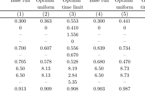
In columns 2 and 5 of Table 2, we report the results of determining the optimal uniform replacement rate. The optimal replacement rate in the baseline economy is around 36 percent. A higher replacement rate reduces search incentives and incentives for wage restraint, so unemployment in-creases. With the optimal uniform replacement rate, unemployment rises to reach 8.1 percent. Individuals living in the baseline economy would be willing to pay 0.33 percent of consumption to move from a replace-ment rate of 30 percent to an optimal uniform one. The optimal uniform replacement rate in the “less flexible” economy is higher since the cost of raising the replacement rate in terms of reducing search incentives is lower. The replacement rate equals 44 percent in the lessflexible economy
Table 2: Numerical results without monitoring and sanctions Baseline economy Lessflexible economy Base run Optimal Optimal Base run Optimal Optimal
uniform time limit uniform time limit
(1) (2) (3) (4) (5) (6) b 0.300 0.363 0.553 0.300 0.441 0.557 p 0 0 0.410 0 0 0.305 µ — — 1.556 — — 1.199 σ — — 0 — — 0 se 0.700 0.607 0.556 0.839 0.734 0.715 ss — — 0.670 — — 0.774 θ 0.705 0.578 0.528 0.680 0.470 0.446 u (%) 6.50 8.13 8.19 6.50 8.73 8.75 ue (%) 6.50 8.13 2.84 6.50 8.73 3.36 us (%) — — 5.35 — — 5.39 w 0.913 0.909 0.908 0.903 0.987 0.896 t (%) 2.09 3.21 3.61 2.09 4.22 4.70 ∆W (%) — 0.33 0.54 — 0.90 1.01
and unemployment increases to 8.7 percent. Individuals in the lessflexible economy would be willing to pay 0.9 percent of consumption in order to live in the optimal uniform system.10
The characteristics of the optimal system with time limits are given in columns 3 and 6. In the baseline economy, benefit differentiation is sub-stantial and the duration of UI benefit receipt is fairly short — the value of µ translates to an expected duration of around two months. The UI replacement rate amounts to 55 percent of the wage; the penalty associ-ated with the loss of entitlement is around 41 percent. The benefit sys-tem with limited duration is substantially more generous than the syssys-tem with infinite duration; with finite duration, unemployment expenditure per non-employed equals 40.5 percent. When search is less elastic, the UI replacement rate is about the same (58 percent) as in our base case. How-ever, the penalty associated with loosing entitlement is decidedly smaller (31 percent), and the expected duration of UI receipt is longer (around
1 0Notice that one should not compare the values of the consumption taxes across the
11 weeks). The unemployment rate is only marginally higher than in the uniform system.
Because the government has two additional instruments (µ and p) besidesb it is not surprising that the welfare gain in the exogenous time limit case exceeds the welfare gain in the optimal uniform case in both economies. The relative gain of introducing time limits is, however, smaller in the lessflexible economy than in the baseline economy. Also note that unemployment goes up by moving from the optimal uniform system to exogenous time limits. In other words, unemployment is not a sufficient statistic for welfare in this case.
4.2
Monitoring and sanctions
This section evaluates the case for monitoring and sanctions and calculates the optimal monitoring and sanctions system. We also discuss the trade-off between monitoring and sanctions and investigate whether the penalties and sanctioning rates generated by the model are in broad conformity with the data.
4.2.1 Are monitoring and sanctions optimal?
The argument in favor of monitoring and sanctions hinges crucially on the costs of this system. Unfortunately, the cost associated with monitoring and sanctions is something of a black box. Therefore, we give an upper bound on the marginal cost below which monitoring and sanctions are an ingredient of the optimal system. Since this upper bound turns out to be very high, we go on to characterize the optimal UI system with monitoring and sanctions.
Is it optimal to introduce monitoring and sanctions? In proposition 2 we stated the condition when the introduction of monitoring and sanctions represents a welfare improvement. For the introduction of monitoring and sanctions to be a welfare improvement relative to the case with time limits,c0(0) has to be less than the gain as represented by greater search incentives among UI recipients with monitoring. We have calculated the cut-off value for our two economies. In our base case, this cut-off value (ˆc) equals ˆc= 0.076; in the alternative case, we have ˆc= 0.047. Both of these numbers have to be considered extremely high. Since the marginal product of labor and the labor force are normalized to unity, we can relate these cut-offvalues to (private sector) GDP by dividing by the employment
rate (which is around 92 percent in the optimal system with time limits). So, the calculated cut-offvalues suggest that as long as the marginal cost is no greater than 4.7/0.92 = 5.1 (7.6/0.92 = 8.3) percent of GDP, it is optimal to introduce monitoring and sanctions. Since these numbers are very large, the introduction of monitoring and sanctions is most likely a welfare improvement relative to the case with time limits.
What is the optimal design of a monitoring and sanctions system? This clearly depends on the exact form of the cost function c(σ). Assume that
c(σ)takes the form ofc(σ) =δσ. To estimate a reasonable value forδ, we used Swedish data on the relative number of employees at the Public Em-ployment Service (PES), since PES officers are responsible for monitoring job search in Sweden. We also used information on how often each PES employee meets a particular unemployed, and the fraction of total time that the PES officer spends in meetings with the unemployed. This calcu-lation, which is presented in greater detail in Appendix B, suggests that the marginal cost of monitoring is in the order of c(σ) = δσ = 0.00785. Provided that σ ≥0.785 in Sweden, then δ = 0.01 is a conservative esti-mate. We also conduct an alternative calculation where δ = 0.02. Note that in both cases δ < ˆc and hence monitoring and sanctions improve welfare.
Table 3 presents some numbers that correspond to the optimal systems in each economy for the two values ofδ. The optimal system involvesσ = 1
given our assumption σ ∈ [0,1]. This particular result should be taken with a due grain of salt given the uncertainty about the costs of monitoring and the properties of the inspection technology. It is nevertheless inter-esting to note that a system with monitoring and sanctions are associated with non-trivial welfare gains relative to the alternatives characterized in Table 2. The relative gain of designing an optimal system with monitoring and sanction is roughly similar in the two economies. Also note that the optimal replacement rate in UI is higher when we introduce monitoring and sanctions. Both economies experience a slight fall in unemployment as compared to Table 2, a result driven by a substantial increase in search effort among the unemployed (particularly those eligible for UI who now face additional incentives to search). Finally, note that the fraction of unemployed with a sanction is considerably lower in Table 3 than in the columns with exogenous time limits in Table 2. Less people need to be penalized in a monitoring system in order to get similar welfare and search incentive effects.
Table 3: Numerical results with monitoring and sanctions Baseline economy Lessflexible economy
δ = 0.01 δ= 0.02 δ= 0.01 δ = 0.02 (1) (2) (3) (4) b 0.626 0.617 0.619 0.610 p 0.564 0.584 0.511 0.570 µ 1.207 1.039 1.017 0.757 σ 1 1 1 1 se 0.755 0.746 0.856 0.848 ss 0.737 0.753 0.842 0.863 θ 0.407 0.408 0.371 0.373 u (%) 7.87 7.88 8.47 8.48 ue (%) 5.75 5.96 7.07 7.37 us (%) 2.12 1.92 1.40 1.11 w 0.906 0.906 0.894 0.894 t(%) 4.60 4.66 5.33 5.35 ∆W (%) 1.15 1.08 1.45 1.38
Table 3 indicates that the trade-offbetween monitoring and sanctions depends on the costs of monitoring: the higher the cost, the lower the mon-itoring rate and the higher the penalty. We have examined this trade-offin greater detail. In particular we have calculated optimal combinations ofµ
andpfor different values ofδ, whereδ is varied from zero to (implausibly) large numbers. We setσ= 1and allowb to adjust optimally. In order to approach the Beckerian corner solution (µ→0,p→1), monitoring costs need to be extremely high. For example, ifδ = 0.14 the optimal system in the baseline economy featuresp= 0.929and µ= 0.234. Risk aversion in combination with a random monitoring technology implies that it is generally not optimal to impose the maximal sanction.
4.2.2 A brief look at the data
Having calculated the optimal systems with monitoring and sanctions it is tempting to relate the predictions of the model to the data. Some of the parameters of the monitoring and sanctions system are of course unob-servable. However, there are observations on the UI replacement rates, the penalties for violating search requirements, and the associated sanctioning
rates. Presumably, there is a lot of noise in the data pertaining to sanction rates. Nevertheless, there is great variation in these data as is clear from Grubb (2001). It seems that the US and Switzerland are the extreme cases in terms of having systems with a large number of sanctions. In the US in the late 1990s, around 10 percent of beneficiaries were sanctioned each quarter for behavior during the benefit period. In addition, some 25 per-cent of the (stock of) eligible unemployed were “sanctioned” because they exhausted their benefits.11 Based on these data, the quarterly sanction rate in the US would be in the order of 35 percent. With the exception of Switzerland, sanctions during the benefit period are substantially less common in the European countries; in fact, the sanction rates are typically lower than one percent per quarter. See Grubb (2001) for further details. The number of sanctions seems to be inversely related to the severeness of the penalty. In the US, the normal sanction for a job search infringement is a loss of benefits for one week.12 In Sweden, on the other hand, the penalty until recently was the loss of benefits for twelve weeks.13
What does the model have to say about the number of sanctions? Figure 1 addresses this question by plotting the sanctioning rates against
σ and assumingδ = 0.01. In addition to the baseline and the less flexible economy, we also consider an economy with low turnover.14 Sanctioning rates decline inσ for two reasons: firstly, for givense, a rise inσ reduces
π(se) ;and, secondly, a rise inσ raises se.
Whenσ = 1, as is optimal given our assumptions, the quarterly sanc-tion rates hover between 10 and 30 percent depending on the exact as-sumptions; see Table 4. The number of sanctions in the baseline economy best conform to sanctioning data for the US. To get at the numbers for the typical European country, it appears that one would have to apply a
1 1This estimate is a crude average for the period 1995-2000. The number of
exhaus-tions per quarter amounted to some 600 000 individuals, the number of unemployed to 6.5 millions, and the fraction eligible for UI to 35 percent. Source: US Department of Labor (labor force statistics and UI program statistics).
1 2Notice, though, that there is a rather harsh ”penalty” associated with the expiration
of UI benefits in the US. In 1991, benefits were reduced by more than 60 percent when benefits expired and the individual was forced to claim welfare benefits instead; see Wang and Williamson (1996).
1 3
The Swedish system has recently been changed in the direction of smaller penalties.
1 4The “low turnover” economy has a lower job destruction rateφ(around 22 percent
per year) and higher value forain the matching function to keep unemployment at the baseline value of 6.5 percent.
0 0.2 0.4 0.6 0.8 1 1.2 1.4 1.6 1.8 0 0.1 0.2 0.3 0.4 0.5 0.6 0.7 0.8 0.9 1 Baseline Less flexible Low turnover
Precision of inspection technology
Figure 1: Quarterly sanction rates,δ = 0.01
Table 4: Quarterly sanction rates according to the model
Baseline economy Lessflexible economy Low turnover economy
δ= 0.01 0.296 0.146 0.242
combination of less elastic search, lower turnover, and higher monitoring costs.
5
Concluding remarks
In this paper we have analyzed the design of optimal unemployment in-surance in a search equilibrium framework where search effort among the unemployed is not perfectly observable. We have examined to what extent the optimal policy should involve monitoring of search effort and benefit sanctions if observed search is found insufficient. The results suggest that the introduction of a system with monitoring and sanctions represents a welfare improvement for reasonable values of the monitoring costs. Those costs would have to be implausibly high — higher thanfive percent of GDP — for this conclusion not to hold.
The policy prescription following from our analysis is thus different from Becker’s (1968) well known result, where the penalty should be max-imal and the probability of getting caught should be close to zero. There are two key assumptions delivering our results. First, individuals are risk averse and, second, monitoring is imperfect. With imperfect monitoring some individuals will be sanctioned even though they search to rule and giving them the maximal penalty is not optimal with risk aversion.
While we are reasonably comfortable in saying that monitoring and sanctions represent a welfare improvement, it is much more difficult to give clear advice on the characteristics of such a system. The reason for this conclusion is that the exact formulation of the monitoring and sanctions system depends on the cost of running such a system. Unfortunately, the cost of running the system is something of a black box.
An issue that we have not addressed is the possibility that formal search requirements may induce individuals to use formal rather than in-formal search methods and therefore bring little increase in total search intensity. Nevertheless, it is likely thatgeneral search requirements — such as the number of job applications filed during a week — should minimize the risk of substitution between search channels. Presumably, substitution is going to be more severe in systems where search requirements are linked to formal channels such as referrals by the public employment service. On this account, therefore, search requirements specified in terms of indepen-dent job search, as used in the US, the Netherlands and Switzerland, seem to be preferable.
Appendix A: The sanctioning probability
This appendix addresses the “structural” interpretation of our sanctioning probability: π(se) = 1−σse. Suppose, realistically, that benefit adminis-trators observe search with error: seo =se+ε, ε∈[εL, εU]. Sincese∈[0,1]
then so shouldseo. This in turn implies restrictions onεL, εU. Ifseo ∈[0,1],
it must be true thatεL=−se and εU = 1−se.
Let us introduce a parameter that indexes the extent of observation error. In particular let ε ∈[−(1−σ˜)se,(1−σ˜)(1−se)]. If σ˜ = 1, there is no observation error. If σ˜ = 0, observed search belongs to the entire admissible range. Suppose also thatε is uniform. Then σ˜ = 0 is a com-pletely random inspection technology. We think of˜σ as a parameter that the central government can invest resources in improving.
An individual is sanctioned wheneverse
o ≤R, whereR∈[0,1]denotes
the search requirement. The probability of being sanctioned given that the individual suppliesse units of search is then
π= Z R−se εL 1 εU−εL dε= R−s e εU−εL − εL εU−εL
SinceεU−εL= 1−˜σ and εL=−(1−σ˜)se, we get
π= R 1−˜σ − ˜ σ 1−σ˜s e
Now we want to impose some restrictions on the parameters of the inspections technology (R,σ˜) to make sure thatπ ∈[0,1]for allse∈[0,1]. We impose the following conditions
1. Ifse= 0thenπ= 1.
2. Ifse= 1thenπ∈[0,1].
The first condition gives R = 1−σ˜. Given R = 1−σ˜, the second condition yieldsσ˜∈[0,0.5]. The conditions we impose on the parameters thus imply that an individual who searches full time is sanctioned with positive probability, i.e., there is a probability of making Type II errors for all values ofse.
In sum, the above assumptions lead to the following formulation for π
π = 1− σ˜
1−σ˜s
e, σ˜
or alternatively, definingσ = ˜σ/(1−σ˜)
π = 1−σse, σ∈[0,1]
Appendix B: Estimating the marginal cost of
mon-itoring
To obtain a reasonable value for the cost of monitoring an additional individual (c(σ)) we performed the following calculation. We relied on data from Sweden, where PES administrators are responsible for monitor-ing whether unemployed individuals have searched to rule or not. Three sources of information were used: (i) the relative number of employees at the PES; (ii) the fraction of time that a PES officer meets with the un-employed; and (iii) the number of contacts between the PES officer and a particular unemployed individual. Information pertaining to items (ii) and (iii) is taken from Lundin (2000).
In the main text the total cost of the monitoring and sanctions system was specified as: C = c(σ)µuew. To get an approximate value for C we start be calculating the wage bill paid to individuals involved in monitor-ing. Since the labor force and the marginal product of labor are normalized to unity, the wage bill is measured relative to these items. The PES service employs approximately 10,000 individuals in Sweden, which translates to around 0.25 percent of the labor force. On average PES officers spend 30 percent of their time in meetings with the unemployed. Assuming that the unemployed are monitored each time they meet with a PES officer we have
C= 0.0025×0.3w= 0.00075w. Thus we haveC=c(σ)µuew= 0.00075w. Turning to the left-hand side of this equation, we set the number of un-employed individuals eligible for UI to 5 percent. With this assumption, we only need an estimate of µ to get an estimate of c(σ). The informa-tion used to estimate µ is derived from a question put to PES officers regarding the number of meetings with individuals searching for a job. When asked about their contact frequency, 35 percent of PES officers an-swered “at most once a month”; 34 percent anan-swered “at most once every other month”; and 31 percent answered “at most once every quarter”. Thus on average a PES officer has (1×0.35 + 0.5×0.34 + 0.31/3)×3 = 1.91 meetings with a particular unemployed per quarter. Hence we have
c(σ) = 0.00075/(µue) = 0.00075/(1.91×0.05) ≈ 0.00785. There is still one unknown in this equation, however; the estimated value ofc(σ) per-tains to a given value of σ. Assuming that c(σ) = δσ, we have δ = 0.01
References
Abbring, J.H., G.J. van den Berg and J.C. van Ours (1997) The effect of unemployment insurance sanctions on the transition rate from unemployment to employment, Working Paper, Tinbergen Institute, Amsterdam.
Becker, G. (1968) Crime and punishment: An economic approach, Jour-nal of Political Economy, 76, 169-217.
Benus, J., J. Joesch, T. Johnson and D. Klepinger (1997) Evaluation of the Maryland unemployment insurance work search demonstra-tion: Final report, Batelle Memorial Institute in association with Abt Associates Inc (http://wdr.doleta.gov/owsdrr/98-2/).
Black, D., J. Smith, M. Berger and B. Noel (1999) Is the threat of train-ing more effective than traintrain-ing itself? Experimental evidence from the UI system, manuscript, Department of Economics, University of Western Ontario.
Boone, J. and J. van Ours (2000) Modeling financial incentives to get unemployed back to work, Discussion Paper 2000-02, CentER for Economic Research, Tilburg University.
Broersma, L. and J.C. van Ours (1999) Job searchers, job matches and the elasticity of matching, Labour Economics, 6, 77-93.
Cahuc, P. and E. Lehmann (2000) Should unemployment benefits de-creases with the unemployment spell?,Journal of Public Economics, 77, 135-153.
Fredriksson, P. and B. Holmlund (2001) Optimal unemployment insur-ance in search equilibrium,Journal of Labor Economics,19, 370-399. Garoupa, N. (1997) The theory of optimal law enforcement, Journal of
Economic Surveys, 11 267-295.
Grubb, D. (2001) Eligibility criteria for unemployment benefits, inLabour Market Policies and Public Employment Service, OECD.
Hopenhayn, H.A. and J.P. Nicolini (1997) Optimal unemployment insur-ance, Journal of Political Economy, 105, 412-438.
Hosios, A.J. (1990) On the efficiency of matching and related models of search and unemployment,Review of Economic Studies, 57, 279-298. Johnson, T. and D. Klepinger (1994) Experimental evidence on unem-ployment insurance work-search policies, Journal or Human Re-sources, 29, 695-717.
Lalive, R., J.C. van Ours and J. Zweimüller (2002) The effect of benefit sanction on the duration of unemployment, Discussion Paper 3311, Centre for Economic Policy Research.
Lundin, M. (2000) Tillämpningen av arbetslöshetsförsäkringens regelverk vid arbetsförmedlingarna, stencil 2000:1, Office of Labour Market Policy Evaluation (IFAU), Uppsala.
Mortensen, D.T. (1977) Unemployment insurance and job search deci-sions,Industrial and Labor Relations Review, 30, 505-517.
Pissarides, C.A. (1990)Equilibrium Unemployment Theory, Basil Black-well, Oxford.
Polinsky, A.M. and S Shavell (1979), The Optimal Tradeoffbetween the Probability and Magnitude of FinesAmerican Economic Review 69, 880-891.
Polinsky, A.M. and S. Shavell (2000) The economic theory of public en-forcement of law,Journal of Economic Literature, 38, 45-76.
OECD (2001) Labour Market Policies and Public Employment Service, Paris.
Shavell, S. and L. Weiss (1979) The optimal payment of unemployment insurance benefits over time,Journal of Political Economy, 87, 1347-1363.
van den Berg, G.J., B. van der Klaauw and J.C. van Ours (1998) Puni-tive sanctions and the transition rate from welfare to work, Discus-sion Paper 9856, CentER for Economic Research, Tilburg University. Forthcoming inJournal of Labor Economics, 2004.
van den Berg, G.J. and B. van der Klaauw (2001) Counseling and mon-itoring of unemployed workers: Theory and evidence from a con-trolled social experiment, Working Paper 2001:12, Institute for Labour Market Policy Evaluation (IFAU), Uppsala.
Wang, C. and S. Williamson (1996) Unemployment Insurance with Moral Hazard in a Dynamic Economy, Carnegie-Rochester Conference Se-ries on Public Policy 44, 1-41.
Publication series published by the Institute for Labour
Market Policy Evaluation (IFAU) – latest issues
Rapport (some of the reports are written in English)
2002:1 Hemström Maria & Sara Martinson ”Att följa upp och utvärdera
arbetsmark-nadspolitiska program”
2002:2 Fröberg Daniela & Kristian Persson ”Genomförandet av aktivitetsgarantin”
2002:3 Ackum Agell Susanne, Anders Forslund, Maria Hemström, Oskar
Nord-ström Skans, Caroline Runeson & Björn Öckert “Follow-up of EU’s re-commendations on labour market policies”
2002:4 Åslund Olof & Caroline Runeson “Follow-up of EU’s recommendations for
integrating immigrants into the labour market”
2002:5 Fredriksson Peter & Caroline Runeson “Follow-up of EU’s
recommenda-tions on the tax and benefit systems”
2002:6 Sundström Marianne & Caroline Runeson “Follow-up of EU’s
recommenda-tions on equal opportunities”
2002:7 Ericson Thomas ”Individuellt kompetenssparande: undanträngning eller
komplement?”
2002:8 Calmfors Lars, Anders Forslund & Maria Hemström ”Vad vet vi om den
svenska arbetsmarknadspolitikens sysselsättningseffekter?”
2002:9 Harkman Anders ”Vilka motiv styr deltagandet i arbetsmarknadspolitiska
program?”
2002:10 Hallsten Lennart, Kerstin Isaksson & Helene Andersson ”Rinkeby Arbets-centrum – verksamhetsidéer, genomförande och sysselsättningseffekter av ett projekt för långtidsarbetslösa invandrare”
2002:11 Fröberg Daniela & Linus Lindqvist ”Deltagarna i aktivitetsgarantin”
Working Paper
2002:1 Blundell Richard & Costas Meghir “Active labour market policy vs
em-ployment tax credits: lessons from recent UK reforms”
2002:2 Carneiro Pedro, Karsten T Hansen & James J Heckman “Removing the veil
of ignorance in assessing the distributional impacts of social policies”
2002:3 Johansson Kerstin “Do labor market programs affect labor force
participa-tion?”
2002:4 Calmfors Lars, Anders Forslund & Maria Hemström “Does active labour
2002:5 Sianesi Barbara “Differential effects of Swedish active labour market pro-grammes for unemployed adults during the 1990s”
2002:6 Larsson Laura “Sick of being unemployed? Interactions between
unem-ployment and sickness insurance in Sweden”
2002:7 Sacklén Hans “An evaluation of the Swedish trainee replacement schemes”
2002:8 Richardson Katarina & Gerard J van den Berg “The effect of vocational
employment training on the individual transition rate from unemployment to work”
2002:9 Johansson Kerstin “Labor market programs, the discouraged-worker effect,
and labor force participation”
2002:10 Carling Kenneth & Laura Larsson “Does early intervention help the
unem-ployed youth?”
2002:11 Nordström Skans Oskar “Age effects in Swedish local labour markets”
2002:12 Agell Jonas & Helge Bennmarker “Wage policy and endogenous wage
rigidity: a representative view from the inside”
2002:13 Johansson Per & Mårten Palme “Assessing the effect of public policy on
worker absenteeism”
2002:14 Broström Göran, Per Johansson & Mårten Palme “Economic incentives and
gender differences in work absence behavior”
2002:15 Andrén Thomas & Björn Gustafsson “Income effects from market training
programs in Sweden during the 80’s and 90’s”
2002:16 Öckert Björn “Do university enrollment constrainsts affect education and
earnings? ”
2002:17 Eriksson Stefan “Imperfect information, wage formation, and the
employ-ability of the unemployed”
2002:18 Skedinger Per “Minimum wages and employment in Swedish hotels and
restaurants”
2002:19 Lindeboom Maarten, France Portrait & Gerard J. van den Berg “An
econo-metric analysis of the mental-health effects of major events in the life of older individuals”
2002:20 Abbring Jaap H., Gerard J. van den Berg “Dynamically assigned treatments:
duration models, binary treatment models, and panel data models”
2002:21 Boone Jan, Peter Fredriksson, Bertil Holmlund & Jan van Ours “Optimal
unemployment insurance with monitoring and sanctions”
Dissertation Series
2002:1 Larsson Laura “Evaluating social programs: active labor market policies and
social insurance”
2002:2 Nordström Skans Oskar “Labour market effects of working time reductions
and demographic changes”
2002:3 Sianesi Barbara “Essays on the evaluation of social programmes and
educa-tional qualifications”
2002:4 Eriksson Stefan “The persistence of unemployment: Does competition