Volatility forecasting using the GARCH framework on the OMXS30 and MIB30 stock indices

(1)

Department of Economics

School of Business, Economics and Law Gothenburg University

Volatility forecasting using the GARCH framework on the

OMXS30 and MIB30 stock indices

Bachelor Thesis 15 credits Winter 2008 Supervisor: Jens Madsen Author: Peter Johansson

(2)

2

Executive Summary

Title

Volatility forecasting using the GARCH framework on the OMXS30 and MIB30 stock indices

Subject

Bachelor Thesis in Financial Economics (15 credits) at the School of Business, Economics and Law, Gothenburg University

Author

Peter Johansson

Supervisor

Jens Madsen, Department of Economics, Gothenburg University

Key Words

Volatility forecasting, Random Walk, Moving Average, Exponentially Weighted Moving Average, GARCH, EGARCH, GJR-GARCH, APGARCH, volatility model valuation, regression, information criterion

Problem

There are many models on the market that claim to predict changes in financial assets as stocks on the Stockholm stock exchange (OMXS30) and the Milano stock exchange index (MIB30). Which of these models gives the best forecasts for further risk management purposes for the period 31st of October 2003 to 30th of December 2008? Is the GARCH framework more successful in forecasting volatility than more simple models as the Random Walk, Moving Average or the Exponentially Weighted Moving Average?

Purpose

The purpose of this study is to find and investigate different volatility

forecasting models and especially GARCH models that have been developed during the years. These models are then used to forecast the volatility on the OMXS30 and the MIB30 indices. The purpose of this study is also to find the model or models that are best suited for further risk management purposes by running the models through diagnostics checks.

Method

Daily prices together with the highest and lowest prices during one trading day for the OMXS30 and MIB30 indices were collected from Bloomberg for the period 31st of October 2003 to 30th of December 2008. These data were then processed in Microsoft Excel and Quantitative Micro Software EViews to find the most successful model in forecasting volatility for each of the two indices. The forecasting was performed on-step ahead for the period 1st of July 2008 to 30th of December 2008.

Results

This study has examined the forecasting ability of various models on the OMXS30 and MIB30 indices. The models were the Random Walk (RW), the Moving Average (MA), the Exponentially Weighted Moving Average (EWMA), ARCH, GARCH, EGARCH, GJR-GARCH and APGARCH. The results suggest that the best performing model was EGARCH(1,1) for both indices.

(3)

3

Acknowledgements

I would like to acknowledge my friend Linus Nilsson currently working for RMF Investment Management in New York for supplying me with the stock indices data and for giving me thoughtful insights in the volatility forecasting area.

I would also like to thank my mother Anita for supporting me and encouraging me during the many hours spent in writing this paper.

Finally, I extend my thanks to my supervisor Jens Madsen at the department of economics, Göteborg University for his support during the writing process. Without him this paper would not have been finished.

(4)

4

Appendix 1 – AIC results for the mean equation Appendix 2 – AIC results of the GARCH(p,q) model Appendix 3 – AIC results of the EGARCH(p,q) model Appendix 4 – AIC results of the GJR-GARCH(p,q) model Appendix 5 – AIC results of the APGARCH(p,q) model Appendix 6 – ARCH LM test for the GARCH models

Appendix 7 – Estimated parameters for the best fitted GARCH models for the OMXS30 index Appendix 8 – Estimated parameters for the best fitted GARCH models for the MIB30 index Appendix 9 – Forecasted volatility with the range as a proxy for the OMXS30 index

(6)

6

1

Introduction

The paragraphs in the introduction section give a brief description of the background, problem definition, delimitations and purpose of this study. The disposition of this report is also presented.

1.1

Background

Trading in the world’s financial markets has increased dramatically over the years. As larger and larger volumes are handled by investors, financial institutions and their traders, it has become more important to handle and evaluate risk. Evidence in the past has showed that lack of risk handling and control systems can have a devastating outcome. An example of lack of risk evaluation is told by the outcomes of the United Kingdom’s oldest merchant bank, Barings Bank. Here one person traded with financial instruments for vast amount of money without risk handling. The result was that the Barings Bank went bankrupt and the total losses exceeded one billion dollars.

Financial instruments are today more exposed to volatility when global markets are

connected to each other and tend to shift rapidly. Financial instruments are also becoming more complex and harder to understand. Therefore investors are paying more interest to the actual risk involved and not only the payoff (Simons, 2000).

Another perspective of risk in classic portfolio theory says that investors can eliminate asset- specific risk by diversifying their portfolio by holding many different assets. Although the risk can be diversified away in this manner, the market does not reward such portfolio handling. Instead an investor should hold a combination of a risk-free asset and the market portfolio. The conclusion here is that investors should not waste resources as investors don’t care about firm-specific risk (Christoffersen, 2003). Many investors have however learnt that firm-specific risk shall have a high priority. Firm-specific risk involves bankruptcy costs, taxes paid which influence the value of the firms, capital structure and the cost of capital. All these risks influence firm value on the market and have a direct influence on the volatility of their stock value.

Many models have been developed over the years to forecast the volatility and thus to give a framework to manage risk. The RiskMetrics model, also called the exponential smoother, was one of the most famous models developed by J P Morgan. Another famous model is the Random Walk. These models are easy to use but have some shortcomings. The

disadvantages with RiskMetrics or the Random Walk have been to drive the development of new models to give a better prediction of future volatility. A set of new models that have been developed are called GARCH, generalized autoregressive conditional heteroskeda-sticity. These models have showed enough flexibility to accommodate specific aspects of individual assets, while still being simple to use (Christoffersen, 2003).

1.2

Purpose

Firstly, the purpose of this study is to find and investigate different volatility forecasting models, especially GARCH models, which have been developed over the years. These models are then used to predict the volatility on the Stockholm stock exchange index (OMXS30) and the Milano stock exchange index (MIB30). Secondly, the aim is to run these models through

(7)

7 diagnostics checks to determine the model or models that are best suited for further risk management purposes.

1.3

Problem definition

There are many models on the market that claim to predict changes in financial assets as stocks on the OMXS30 and MIB30 indices. Which of these models gives the best predictions for further risk management purposes for the period 31st of October 2003 to 30th of

December 2008? Is the GARCH framework more successful in predicting volatility than more simple models such as the Random Walk, Moving Average or the Exponentially Weighted Moving Average models?

1.4

Delimitations

The study presented in this report is limited to volatility forecasting on the Stockholm stock exchange index (OMXS30) and the Milano stock exchange index (MIB30). Models studied are the Random Walk (RW), the Moving Average (MA), the exponentially weighted Moving Average (EWMA), ARCH, GARCH, EGARCH, GJR-GARCH and APGARCH. The estimations of the models are performed under the assumption that the returns of the stock indices follow the normal distribution. No estimation is used under the assumption of a Student-t distribution, Skewed Student-t distribution, Gereralized Error Distribution or any other distribution. Furthermore, processing of the forecasted data as Value at Risk (VaR) or Expected Shortfall (ES) is not performed in this study.

The time period used for the data from the stock indices range from 31st of October 2003 to 30th of December 2008.

1.5

Disposition

The report starts with chapter 1 introducing the subject, the purpose of the study, the problem definitions and the delimitations. It then continues with chapter 2 explaining the methodology and approach to the study. In chapter 3 the theoretical framework goes through the theories used to retrieve the results. Chapter 4 describes the data and the data processing methodology. The results found are then presented in chapter 5 followed by an analysis and discussion in chapter 6. Chapter 7 gives some final thoughts and summarises the study. Further research suggestions of subjects not covered in this study are presented in chapter 8. Finally, the report ends with a list of references used when writing this report.

2

Methodology

The paragraphs in the methodology section describe the type of study that is performed in this report. The approach to the study is also described.

2.1

Choice of methodology

There are traditionally two methods used when investigating problems similar to problems in this report. They are the qualitative and quantitative studies. When using a qualitative study a limited number of units are investigated to gain a deeper understanding of these units. A qualitative study most likely leads to a situation where the researcher’s

comprehension or interpretation of the information found serves as a basis for the results found in the study.

(8)

8 When using a quantitative study a vast number of units are studied with the purpose of gaining knowledge on a limited number of factors for each unit. Statistical analysis is most likely to take place of the data of interest such that different phenomenon can be explained using a selection of a certain population. A quantitative study can also be used to generalize and to represent other units in a similar population (Holme and Solvang, 1996).

The presented problems and the data used to find the results in this study use a quantitative methodology. It is possible to generalize the studied problems to similar populations (stock indices) and the results are based on statistical analysis of the collected data. A quantitative methodology to the study thus makes sense.

2.2

Approach to the study

In general there are two main approaches to data in a study. These approaches are the deductive approach and the inductive approach. When using a deductive approach the conclusions made for specific events are based on general principles and existing theories. Based on these known theories and principles hypothesis are derived and then further empirically tested for the cases studied. The choice and interpretation of data used are also influenced by the known theories and principles.

When using an inductive approach specific events are not derived from hypothesis derived from existing theories. The events are here studied without prior knowledge or influence of theories. A new theory is compiled and formulated using the results of the study (Davidsson, Patel, 1994).

The study presented in this report uses a deductive approach. Academic research in the field has been performed during several years investigating similar problems. Practices based on these investigations have been prepared and made accessible for the general public. A deductive approach in this case thus makes sense.

3

Theoretical framework

The paragraphs in the theoretical framework describe the theories used to form the results in this study.

3.1

Asset returns, volatility and standard deviation

The return of an asset today is defined as the difference between the closing price of the asset today and its closing price yesterday divided by yesterday’s closing price.

𝑅_𝑡+1 = 𝑆𝑡+1 − 𝑆𝑡 𝑆_𝑡

(1)

The log return is used widely as the output of the calculation is unit free. Log returns are thus suitable for comparison with other unit free returns. The return or daily geometric return, also called “log” return can be defined as the change in the logarithm of daily closing prices of an asset.

(9)

9 The volatility is a measure of fluctuations in asset returns. An asset has a high volatility when the return fluctuates over a wide rage. When the return fluctuates over a small range the asset has a low volatility. Volatility can be seen as a risk measure or an uncertainty of asset return movements faced by participants in financial markets. The volatility is measured by the volatility or the standard deviation and is a measure of the asset returns dispersion over a specified time period.

𝜎2 ₌ 1

𝑁 − 1 𝑅𝑡 − 𝑅 2

𝑁

𝑡=1

(3) The standard deviation is simply the square root of the volatility.

𝜎 = 1 𝑁 − 1 𝑅𝑡− 𝑅 2 𝑁 𝑡=1 (4) where: 𝜎2 _{is the volatility}

𝜎 is the standard deviation

𝑅𝑡 is the asset return at time t

𝑅 is the average return over the specified time period

𝑁 is the number of days for the specified time period

3.2

Stylized facts of volatility and asset returns

In order to model future volatility or the volatility of assets forming a portfolio or index it is important to consider the stylized facts. These facts have been found through vast academic research and seem to fit for most markets, time periods and types of assets.

1. It can be found that daily returns have very little autocorrelation. Thus, returns are almost impossible to predict by only looking at the past returns.

𝐶𝑜𝑟𝑟 (𝑅𝑡+1, 𝑅𝑡+1−𝜏) ≈ 0 𝑓𝑜𝑟 𝜏 = 1, 2, 3, … , 100 (5)

The correlation of returns with returns lagged from 1 to 100 days of the OMXS30 index and the MIB30 index are shown in Figure 1 and Figure 2. When investigating these graphs it can be argued that the conditional mean fluctuates around zero and is fairly constant.

(10)

10 Figure 1 – Autocorrelations of daily OMXS30

returns

Figure 2 – Autocorrelations of daily MIB30 returns

The unconditional distribution of daily returns usually deviates from normality. This

phenomenon is called excess kurtosis. Figure 3 and Figure 4 show a histogram along with the normal distribution. A closer look tells us that the histograms in these figures have fatter tails and have higher peaks around zero. The tails are usually fatter on the left side of the distribution. Fatter tails to the left of the distribution indicates higher probabilities of large losses compared to losses under the normal distribution. The QQ-plots in Figure 5 and Figure 6 further shows the deviation from normality in the tails.

Figure 3 – Daily OMXS30 returns against the normal distribution

Figure 4 – Daily MIB30 returns against the normal distribution

Figure 5 – QQ-Plots of daily OMXS30 returns against the normal distribution

Figure 6 – QQ-plot of daily MIB30 returns against the normal distribution

(11)

11 2. Stock market movements tend to have more large drops in value than corresponding

large increases. The market is thus negatively skewed. Once again this can be seen in Figure 3 and Figure 4.

3. It is hard to statistically reject a zero mean of return. For short horizons such as daily the standard deviation of returns is given more importance. The OMXS30 index has a daily standard deviation of 1.1644% and a daily mean of 0.0281%. For the MIB30 index the numbers are 0.8804% and 0.0103% respectively.

4. It can be found that volatility measured by squared returns have a positive

correlation with past returns, especially for short horizons such as daily or weekly. Figure 7 and Figure 8 shows the autocorrelation in squared returns for the OMXS30 index and the MIB30 index.

Figure 7 – Autocorrelations of squared daily OMXS30 returns

Figure 8 – Autocorrelations of squared daily MIB30 returns

5. The correlation tends to increase between assets. Especially in bearish markets or during market crashes. This phenomenon is also referred to as volatility clustering where extreme returns are followed by other extreme returns, although not necessarily of the same sign. Figure 9 and Figure 10 shows the returns for the OMXS30 index and the MIB30 index over time where volatility clusters are present.

(12)

12 6. Equity and equity indices tend to have a negative correlation between their volatility

and returns. This phenomenon is called the leverage effect and is due to the fact that a drop in stock price will increase the leverage of a firm under a constant capital structure, i.e. if debt stays constant.

These stylized facts are the most common facts mentioned in academic literatures. Other facts are also present. Regardless, it is important to know how these effects influence the financial data when using models for volatility forecasting. When considering these facts the daily return can be specified (Christoffersen, 2003).

𝑅𝑡+1 = 𝜇𝑡+1 + 𝜀𝑡+1 (6)

𝜀_𝑡+1 = 𝜎_𝑡+1𝑧_𝑡+1 and zt+1∼ i.i.d D(0,1) (7)

The random variable zt+1 is an innovation term which is assumed to be identically and

independently distributed according to the distribution D(0,1). This distribution in this study is assumed to be the normal distribution with a mean equal to zero and volatility equal to one. The conditional mean of the return μt+1 is assumed to be zero (Christoffersen, 2003).

Researchers sometimes include an autoregressive term of the first order AR(1) or a Moving Average term of the first order MA(1) in the mean equation. A combination of these terms of the first order will be an ARMA(1,1) term. Higher orders of these terms AR(p), MA(q), are also possible to include in the mean equation.

𝑅𝑡+1 = 𝜇𝑡+1+ 𝛽𝑖,𝐴𝑅 𝑝 𝑖=0 𝐴𝑅 𝑖 + 𝛽𝑗 ,𝑀𝐴 𝑞 𝑗 =0 𝑀𝐴 𝑗 + 𝜀𝑡+1 (8)

By including these terms the model (mean equation) might capture dynamic features of the data better. The AR term states that a time-series current value depends on its current and previous value of a white noise error term. A time-series linear dependency on its own previous value is captured by the MA term (Brooks, 2008). The terms are selected using the Akaike Information Criterion (AIC), see paragraph 3.5.1.

3.3

Volatility modelling

This study focus on Generalized Autoregressive Conditional Heteroskedastic (GARCH) models that are exploiting different aspects of the stylized facts described in paragraph 3.2 above. The following paragraphs will describe the different GARCH models in more detail. Other more simple models are also described as these are the foundation of the more complex GARCH models.

3.3.1 The Random Walk (RW) model

The Random Walk (RW) model only considers the actual volatility in the present time period as a forecast for the volatility in the following time period. Thus, volatility is almost

impossible to forecast based on historical information as the movement on the stock markets are seen as random.

𝜎_𝑡+12 _{= 𝜎}

(13)

13 where:

𝜎𝑡+12 is the forecasted unconditional volatility based on the actual volatility at time t

𝜎_𝑡2 _{is the unconditional volatility at time t from equation (3) with a 25 day sliding} window, which is the average number of trading days in a month

3.3.2 The Moving Average (MA) model

The Moving Average (MA) model states that if a period in time has a high volatility there is also a high probability of high volatility in the following time periods. Tomorrow’s volatility is thus the simple average of the most recent observations.

𝜎_𝑡+12 ₌ 1 𝑚 𝜎𝑡+1−𝜏2 𝑚 𝜏=1 (10) where:

𝜎_𝑡+12 _{is the forecasted unconditional volatility based on information given at time t}

𝜎_{𝑡+1−𝜏}2 _{is the unconditional volatility at time t+1-τ}

𝑚 is the number of observations

The drawback of this model is that extreme returns will influence the volatility for 1/m times the squared return for m time periods as equal weights are put on all past observations. Another drawback is that it can be difficult to select the number of observations.

3.3.3 The Exponentially Weighted Moving Average (EWMA) model

The Exponential Weighted Moving Average model (EWMA) or the exponential smoother, developed by JP Morgan considers the drawback with equal weights on past observations. Weights on the observations are declining exponentially over the time period. The influence on extreme returns is smoothed out compared to the Moving Average model.

𝜎_𝑡+12 _{= 𝜆𝜎}

𝑡2+ 1 − 𝜆 𝜎𝑡2 (11)

where:

𝜎_𝑡+12 _{is the forecasted conditional volatility based on information given at time t}

𝜆𝜎_𝑡2 _{is the volatility at time t}

1 − 𝜆 𝜎_𝑡2 _{is the is the forecasted unconditional volatility at time t from equation (10)}

𝜆 is the smoothing parameter

The smoothing parameter λ shall be estimated with values ranging from zero to one. When the exponential smoother model was developed it was found that a λ=0,94 was best for most assets for daily data (Jorion, 2001). This value has since then become an industry standard and is also used in this study.

3.3.4 The ARCH(q) model

R F Engle (1982) proposed a model where the conditional volatility was modelled with an AutoRegressive Conditional Heteroscedasticity (ARCH) processes. The term autoregressive

(14)

14 here states that past events influence future events but with diminishing effect as time pass by. Engle used the fact that financial time series usually incorporates clusters of high and low volatility over longer time periods. The time series thus show heteroscedasticity. As the volatility usually is gathered in clusters Engle found no independent variable that explained this phenomenon. He therefore used a regression based model with past squared returns as a describing factor for volatility forecasting. The lag parameter for past squared returns is described with q. The most simplest ARCH(q) process is a ARCH(1) process where the squared return is lagged one time period.

𝜎_𝑡+12 _{= 𝜔 + 𝛼} 𝑖𝜀𝑡+1−𝑖2 𝑞

𝑖=1

(12)

with ω > 0 and 𝛼𝑖 ≥ 0 for all 𝑖 = 1 to 𝑞. where:

𝜔 is a constant

𝛼 is the ARCH coefficient

𝜀_{𝑡+1−𝑖}2 _{is the squared residual from the mean equation at time t+1-i}

𝑞 is the non-negative order of the Moving Average ARCH term

3.3.5 The GARCH(p,q) model

The ARCH model was extended to a Generalized AutoRegressive Conditional

Heteroscedasticity (GARCH) model by Tim Bollerslev (1986). This model not only considers past squared returns but also past volatilities to forecast the volatility. Thus the ARCH model was extended with an autoregressive term q for the volatility. The most simplest GARCH(p,q) process is a GARCH(1,1) process.

𝜎_𝑡+12 _{= 𝜔 + 𝛼} 𝑖𝜀𝑡+1−𝑖2 𝑝 𝑖=1 + 𝛽_𝑗𝜎_{𝑡+1−𝑗}2 𝑞 𝑗 =1 (13)

with ω > 0, 𝛼𝑖 ≥ 0 for all 𝑖 = 1 to 𝑝, 𝛽𝑗 ≥ 0 for all 𝑗 = 1 to 𝑞 and (sum of 𝛼𝑖 + sum of 𝛽𝑗) < 1. where:

𝜎𝑡2 is the volatility at time t

𝜔 is a constant

𝛽 is the GARCH coefficient

3.3.6 The EGARCH(p,q) model

The GARCH(p,q) model does not consider the fact that a drop in asset return has a larger effect on the volatility then a corresponding rise in asset return. This effect is called the

(15)

15 leverage effect and is also argued in stylized fact number six above. The GARCH(p,q) model can be modified to deal with this phenomenon. The Exponential GARCH (EGARCH) model proposed by Nelson (1991) considers the asset returns effect on volatility differently depending on whether the return is positive or negative. An advantage with the model is that the volatility is always positive. The drawback with the model is that the forecasted volatility for lags larger than one cannot be calculated analytically. The most simplest EGARCH(p,q) process is a EGARCH(1,1) process.

log 𝜎_𝑡+12 _{= 𝜔 + 𝛼} 𝑖 𝑝 𝑖=1 𝜀_{𝑡+1−𝑖} 𝜎_{𝑡+1−𝑖} + 𝛾𝑘 𝑟 𝑘=1 𝜀_𝑡−𝑘 𝜎_𝑡−𝑘 + 𝛽𝑗 𝑞 𝑗 =1 𝑙𝑜𝑔 𝜎_{𝑡+1−𝑗}2 ₍₁₄₎

with no restrictions on the parameters since the logarithm prevents 𝜎𝑡+12 to be negative. where:

log 𝜎_𝑡+12 _{is the log forecasted conditional volatility based on information given at time t}

𝜎_{𝑡+1−𝑗}2 _{is the volatility at time t+1-j}

𝜎_𝑡−𝑘 is the standard deviation at time t-k

𝛾 is the leverage coefficient

𝜔 is a constant

𝜀𝑡+1−𝑖 is the squared residual from the mean equation at time t+1-i

𝑝 is the non-negative order of the Moving Average ARCH term

𝑞 is the non-negative order of the autoregressive GARCH term

𝑟 is equal to p

3.3.7 The GJR-GARCH(p,q) model

Glosten, Jagannathan and Runkle (1993) proposed another extension to the GARCH model, which deals with the leverage effect. An indicator variable was here introduced to form the GJR-GARCH model. The indicator variable takes the value 1 if the return at time period t is positive. Otherwise the indicator variable takes the value 0. The most simplest GJR-GARCH (p,q) process is a GJR-GARCH(1,1) process.

𝜎_𝑡+12 _{= 𝜔 + 𝛼} 𝑖 𝑝 𝑖=1 𝜀_{𝑡+1−𝑖}2 + 𝛾𝑘𝜀𝑡+1−𝑘2 𝑟 𝑘=1 𝐼_{𝑡+1−𝑘}− _{+ 𝛽} 𝑗 𝑞 𝑗 =1 𝜎_{𝑡+1−𝑗}2 (15)

with ω > 0, 𝛼𝑖 ≥ 0 for all 𝑖 = 1 to 𝑝, 𝛽𝑗 ≥ 0 for all 𝑗 = 1 to 𝑞, (𝛼𝑖 + 𝛾𝑘) ≥ 0 for all 𝑖 = 1 to 𝑝 and 𝑘 = 1 to 𝑟 and (sum of 𝛼𝑖 + sum of 𝛽𝑗 + 0.5 sum of 𝛾𝑘) < 1 for all 𝑖 = 1 to 𝑝, 𝑗 = 1 to 𝑞 and 𝑘 = 1 to 𝑟.

where:

(16)

16

𝐼_{𝑡+1−𝑘}− _{is an indicator variable that takes the value 1 or 0 at time t+1-k}

𝜔 is a constant

𝑟 is equal to p

3.3.8 The APGARCH(p,q) model

The Asymmetric Power GARCH (APGARCH) model was introduced by Ding, Granger and Engle (1993). It is similar to the GJR-GARCH model as the leverage effect is considered. The difference with the APGARCH models is that it allows the power к to be estimated. The power к usually takes the value 2 (Ding, Granger and Engle (1993)). The most simplest APGARCH(p,q) process is a APGARCH(1,1) process.

𝜎_𝑡+1δ _{= 𝜔 + 𝛼} 𝑖 |𝜀𝑡+1−𝑖| − 𝛾𝑖𝜀𝑡+1−𝑖 𝛿 p i=1 + 𝛽_𝑗𝜎_{𝑡+1−𝑗}δ q j=1 (16)

with δ > 0, |𝛾𝑖| ≤ 1 for all 𝑖 = 1 to 𝑟, 𝛾𝑖 = 0 for all 𝑖 > 𝑟 and 𝑟 ≤ 𝑝. where:

𝜎_𝑡+1δ _{is the forecasted conditional volatility based on information given at time t}

𝜎_{𝑡+1−𝑗}δ _{is the volatility at time t+1-j}

𝛿 is the power coefficient

𝜔 is a constant

𝜀_{𝑡+1−𝑖} is the residual from the mean equation at time t+1-i

The APGARCH model also includes other GARCH models as special cases. If restrictions are set on its parameters the below models can be specified:

 ARCH when 𝛿 = 2, 𝛾𝑖= 0 for all 𝑖 = 1 to 𝑝 and 𝛽𝑗 = 0 for all 𝑗 = 1 to 𝑞  GARCH when 𝛿 = 2, 𝛾𝑖= 0 for all 𝑖 = 1 to 𝑝

 GJR-GARCH when 𝛿 = 2

3.3.9 Other GARCH models

There exist a variety of other GARCH models. The Threshold GARCH (TGARCH) model introduced by Zakoian (1994) and the Quadratic GARCH (QGARCH) model introduced by Sentana (1995) are similar to the GJR-GARCH model. They both consider the leverage effect.

(17)

17 Other models as the Integrated GARCH (IGARCH) or the GARCH in mean (GARCH-M) are models that uses restrictions on the basic GARCH model or uses GARCH terms in the mean equation for the return. More complex GARCH models are the Regime Switching GARCH (RS-GARCH) model introduced by Gray (1996) or the fractionally integrated GARCH model

(FIGARCH) introduced by Baillie, Bollerslev and Mikkelsen (1996), which forecasts volatility at longer time periods than daily or weekly. New GARCH models are proposed continuously but they all origin from the simple ARCH model proposed by Engel (1982). A list of many

proposed models is found in the Glossary to ARCH (GARCH) also called as “alphabet-soup” (Bollerslev, 2008). The GARCH models mentioned in this paragraph will not be dealt with in this study.

3.4

Maximum-Likelihood parameter estimation

The GARCH models described in previous sections contain unknown parameters. These parameters must be estimated in order to fit the GARCH models properly to the historical (in-sample) data used for volatility forecasting. The method used to find the unknown parameters is based on Maximum Likelihood Estimation (MLE).

If equation (6) is considered and the assumption of i.i.d. under the normal distribution, the likelihood or probability that 𝑅𝑡 will occur is defined as 𝑙𝑡 (Christoffersen, 2003).

𝑙_𝑡 = 1

2𝜋𝜎_𝑡2𝑒𝑥𝑝 −

𝑅_𝑡2

2𝜎_𝑡2 (17)

The joint likelihood of all squared returns within the time period is defined as 𝐿.

𝐿 = 𝑙𝑡 𝑇 𝑡=1 = 1 2𝜋𝜎_𝑡2𝑒𝑥𝑝 − 𝑅_𝑡2 2𝜎_𝑡2 𝑇 𝑡=1 (18) The unknown parameters are then selected to fit the data by maximizing the joint log likelihood of all squared returns within 𝐿.

max log 𝐿 = 𝑚𝑎𝑥 𝑙𝑛 𝑙_𝑡 = 𝑚𝑎𝑥 −1 2𝑙𝑛 2𝜋 − 1 2𝑙𝑛 𝜎𝑡2 − 1 2 𝑅_𝑡2 𝜎_𝑡2 𝑇 𝑡=1 𝑇 𝑡=1 (19) where:

𝐿 is the likelihood of all squared asset returns between time t and T

𝑙𝑡 is the likelihood of the squared asset return at time t

𝜎𝑡2 is the volatility at time t

𝑅_𝑡2 _{is the squared asset return at time t}

3.5

Evaluation statistics

Several statistical tests are performed in the software package EViews to determine which volatility models that are most suitable for the data used in the study. This paragraph

(18)

18 describes the Akaike Information Criterion (AIC) and the ARCH Lagrange multiplier (ARCH LM) test.

3.5.1 Akaike Information Criterion (AIC)

Models will fit a time-series as daily data from a stock index with different success depending on their specifications. Information criterion can be used as a guide when

selecting the most appropriate model. The Akaike Information Criterion (AIC) consists of two parts. The first part is a test statistics derived from the maximum likelihood function. A penalty is then calculated in the second part for the loss of degrees of freedom from adding extra parameters (Brooks, 2008). The lower the information criteria the better the model fits the data. 𝐴𝐼𝐶 = −2𝑙 𝑇 + 2𝑘 𝑇 (20) where:

𝐴𝐼𝐶 is the test value

𝑙 is the test statistics derived from the likelihood function

𝑘 is the number of estimated parameters

𝑇 is the number of observations

3.5.2 ARCH Lagrange Multiplier (ARCH LM) test

When using ARCH models for volatility forecasting it is appropriate to test if the time series consists of ARCH effects in the residuals. That is, if there is evidence of autoregressive conditional heteroskedasticity. If there is no evidence, ARCH models are not appropriate for volatility forecasting. The ARCH Lagrange multiplier (ARCH LM) test checks for ARCH effects in the residuals. When the ARCH models have been used and their parameters have been estimated for the in-sample period there should be as little evidence as possible left of any further ARCH effects. If there is still evidence of ARCH effects in the residuals there is more information in higher orders of the model that may explain the volatility better. A regression is used to compute two test statistics. The null hypothesis that there are no ARCH effects in the residuals up to order q is then tested (EViews, 2005).

𝜀𝑡2 = 𝛽0+ 𝛽𝑖 𝑞 𝑖=1 𝜀_𝑡−𝑖2 _{+ 𝑣} 𝑡 (21) where:

𝜀_𝑡2 _{is the squared residual at time t}

𝑘 is the number of estimated parameters

𝛽₀ is the intercept

𝛽_𝑖 is the slope

𝑣_𝑡 is the error term

(19)

19 The two test statistics computed for this test are the F-statistic and the OBS*R-squared test statistic. From these test statistics p-values can be calculated, which is used to check if the null hypothesis can be rejected or not.

3.6

Forecast volatility model evaluation

When the volatility model has been selected and the parameters have been estimated it is necessary to check if the model performs as expected. This paragraph describes the evaluation process based on regression, the R2 test and the F-statistic test.

3.6.1 Out-of-sample check using regression

A volatility model can be evaluated using regression. The squared return for the forecast period 𝑅𝑡+12 is regressed on the volatility forecast from the volatility model itself.

𝑅_𝑡+12 _{= 𝑏}

0 + 𝑏1𝜎𝑡+12 + 𝑒𝑡+1 (22)

where:

𝑅𝑡+12 is the squared asset return at time t + 1

𝑏0 is the intercept

𝑏1 is the slope

𝑒𝑡+1 is the error term

The volatility forecast 𝜎𝑡+12 should be unbiased and efficient. It is unbiased if it has an intercept of 𝑏0 = 0 and efficient if the slope 𝑏1 = 1. It shall be noted that as the squared return shows a high degree of noise the fit of the regression will be fairly low, typically around 5 - 10% (Christoffersen, 2003).

3.6.2 Intraday high and low prices

Instead of using the squared return as a proxy for the volatility the range can be used. The range is the difference between the logarithmic high and low price of an asset during a trading day.

𝐷𝑡 = 𝑙𝑛 𝑆𝑡𝐻𝑖𝑔𝑕 − 𝑙𝑛 𝑆𝑡𝐿𝑜𝑤 (23)

where:

𝐷𝑡 is the range at time t

𝑆_𝑡𝐻𝑖𝑔𝑕 is the highest price of an asset observed during day t

𝑆𝑡𝐿𝑜𝑤 is the lowest price of an asset observed during day t

Peter Christoffersen (2003) suggests that the proxy for the daily volatility shall have the following form.

𝜎𝑟,𝑡2 =

1

(20)

20 As in the out-of-sample check in the previous paragraph, regression is used for evaluating the forecast from the volatility model.

𝜎_𝑟,𝑡2 _{= 𝑏}

0+ 𝑏1𝜎𝑡+12 + 𝑒𝑡+1 (25)

where:

𝜎𝑟,𝑡2 is the range-based estimate of unconditional volatility at time t + 1

𝑏₀ is the intercept

𝑏₁ is the slope

𝑒_𝑡+1 is the error term

3.6.3 Goodness of fit statistic, R2 test

When comparing forecasted models they have to be distinguished in terms of goodness of fit between the data and the model before they can be ranked. The R2 test is such a measure explaining how well a model containing explanatory variables actually explains variations in the dependent variable (Brooks, 2008). In other words to what extent the parameters and variables in the models used in this study explain the forecasted volatility on the OMXS30 and MIB30 stock indices. The R2 test uses regression and will equal 1 if the fit is perfect and 0 if the fit is no better than the mean of the dependent variable (EViews, 2005).

3.6.4 The F-statistic from regression

The F-statistic reported from a regression tests the hypothesis that all slope parameters (bn)

except the constant (c) and the intercept (b0) is zero. That is, if the regressed parameters

includes information from the dependent variable. The reported p-value Prob(F-statistic) is the marginal significance level of the F-test. If the p-value is significant the null hypothesis is rejected and the slope parameters (bn) are significantly different from zero (EViews 2005).

𝐹 = 𝑅2/ 𝑘 − 1

1 − 𝑅2_{/ 𝑇 − 𝑘} (26)

where:

𝐹 is the test value

𝑅2 _{is the goodness of fit statistic}

𝑘 − 1 is the number of numerator degrees of freedom

𝑇 − 𝑘 is the number of denominator degrees of freedom

4

Data and data processing methodology

The paragraphs in the data and data processing methodology section describe the data and the methods used in this study. Data can be divided in primary data and secondary data when used for research purposes. Primary data is data that researchers gather themselves through interviews or observations during the work of the study. Secondary data is data that have already been found by others and that can be extracted from databases, books or journals etc. (Holme and Solvang, 1996). This report only uses secondary data.

(21)

21

4.1

Description of the data

The data consists of daily prices from the OMXS30 and MIB30 indices. Both OMXS30 and MIB30 list the 30 most valued companies on the Stockholm Stock Exchange and the Milano Stock Exchange. The time period for both OMXS30 and MIB30 indices is 31st of October 2003 to 30th of June 2008. That is roughly five years giving 1171 sample points for OMXS30 and 1185 sample points for MIB30. Peter Christoffersen (2003) argues that a general rule of thumb is to use the last 1000 data points for volatility forecasting. The number of sample points differs between the indices due to different number of holidays and different dates when holidays occurs between Sweden and Italy. Included with the daily prices the data also contains the daily range, highest and lowest daily price. The data has been retrieved using the Bloomberg databases.

4.1.1 In- and out-of-sample periods

The RW model only uses the previous sample point of the actual volatility to forecast the volatility. Thus the actual volatility for sample 1171 for the OMXS30 index and 1185 for the MIB30 index is used giving the first forecasted value in the out-of-sample period. The forecasting is then performed one step ahead throughout the out-of-sample period.

𝜎_𝑡+12 _{= 𝜎}

𝑡2 and tOMXS30 = 1172, 1173, ... , 1299 (27)

𝜎_𝑡+12 _{= 𝜎}

𝑡2 and tMIB30 = 1186, 1187, ... , 1312 (28)

For the MA model the moving average window is set to equal the number of sample points in the in-sample period. That is the moving average window for the OMXS30 index is 1171 and 1185 for the MIB30 index. The forecasting is then performed using these sample point sliding windows throughout the out-of-sample period.

𝜎_𝑡+12 ₌ 1 1171 𝜎𝑡+1−𝜏2 1171 𝜏=1 and tOMXS30 = 1172, 1173, ... , 1299 (29) 𝜎_𝑡+12 ₌ 1 1185 𝜎𝑡+1−𝜏2 1185 𝜏=1 and tMIB30 = 1186, 1187, ... , 1312 (30)

The EWMA model only requires 100 lags in order to include 99,8% of all the weights neces-sary to calculate tomorrow’s volatility (Christoffersen, 2003). To forecast the first day of volatility in the out-of-sample period weights 1072 to 1171 are used for the OMXS30 index and weights 1086 to 1185 are used for the MIB30 index. The forecasting is then performed using the 100 sample point sliding windows throughout the out-of-sample period.

𝜎_𝑡+12 _{= 𝜆𝜎}

𝑡2 + 1 − 𝜆 𝜎𝑡2 and tOMXS30 = 1172, 1173, ... , 1299 ₍₃₁₎

𝜎_𝑡+12 _{= 𝜆𝜎}

𝑡2 + 1 − 𝜆 𝜎𝑡2 and tMIB30 = 1186, 1187, ... , 1312 (32) The in-sample period when the coefficients for the ARCH type models are estimated is equal to the time period of the retrieved data, 31st of October 2003 to 30th of June 2008. When the coefficients have been found and fitted to the data using MLE the coefficients are used to

(22)

22 forecast the volatility one day ahead during the period 1st of July 2008 to 30th of December 2008. This period is the out of sample period. The forecasting is thus made in a sliding window one day ahead throughout the out-of-sample period. 1st of July 2008 is the first day of forecasted volatility and 30th of December is the last day of forecasted volatility. Note that the out-of-sample period includes returns with high levels of volatility.

4.2

Criticism of the sources

The quality of the gathered data is very important in order to prevent biased results. It is therefore sound to treat the data with some scepticism. Typical questions to consider are the purpose of the data, when and where the data was gathered or even why the data exists. Further questions to consider are the circumstances when the data was collected, who the originator of the data is and its relation to the data (Davidson and Patel, 1994). The data used for this study is gathered by Bloomberg and used by many institutions and agents in the financial markets. There is no reason to think that this data is not correct or biased in any way for purposes only known by Bloomberg.

4.3

Validity and reliability

When researching a topic it is important that the result reflects the questions asked about the topic. Validity thus ensures that this is fulfilled. Reliability deals with the consistency of a number of measurements and is determined based on the processing of the data. Reliability can be increased if the data is treated carefully to avoid errors. Validity implies reliability, but reliability does not imply validity (Holme and Solvang, 1996).

Bloomberg provides data to professional institutions and agents in financial markets all over the world. They have processes and rules that ensure correct data in their databases. If this were not the case they could not charge users for their services. The data is thus seen as reliable. Methods and calculations used in this study are presented in such a way that they could be replicated. A description and definition of what this study will find is also provided. The study can then be seen as valid.

4.4

Data processing

The data from the two indices are used to calculate other necessary data in order to further study the forecasting models. First, the prices are transformed to returns using equation (2). The actual volatility is computed using equation (3). Each of the MA, EWMA and RW models forecasted volatility are calculated using their respective formulas in paragraph 4.1.1. Finally the range and the range volatility are calculated using equation (23) and (24) respectively. All calculations are performed in Microsoft Excel. The data are then imported to Quantitative Micro Software EViews for further analysis. Note that the forecasting for the ARCH type models are performed in EViews and thus didn’t have to be calculated in Excel.

5

Results

The data in the result paragraphs describe the results found on empirical data. First the mean equation is examined followed by the stylized facts and found model parameters. Then the in-sample results for the different models are presented followed by the forecast and the out-of-sample results of the model valuation.

(23)

23

5.1

The mean equation

The mean specification is found in equation (8). Regression is used to find if an AR(p), MA(q) or ARMA(p,q) term shall be included in the mean equation used by the ARCH type models. The EViews Akaike Information Criterion (AIC) is used to find the best model for the mean equation for the in-sample period. The results are show in Table 4 in Appendix 1. For the OMXS30 index the mean equation shall follow an AR(1) process whereas an ARMA(5,5) process is more suitable for the MIB30 index.

5.2

Statistics of the OMXS30 and MIB30 indices

Evidences of the stylized facts are already discussed in paragraph 3.3. Most of these facts can also be measured statistically. Table 1 shows the result of the sample statistics.

OMXS30 MIB30

Number of observations 1171 1185

Daily mean (%) 0.0281 0.0103

Daily standard deviation (%) 1.1644 0.8804

Zero mean test 0.8246 (0.4098) 0.4030 (0.6870)

Skewness -0.322654 -0.589149

Excess kurtosis 5.073684 5.931765

Jarque-Bera value 229.9337 (<0.001) 492.5258 (<0.001) Ljung-Box Q-statistics (10 lags) 23.688 (0.008) 18.977 (0.041) Ljung-Box Q-statistics (20 lags) 33.799 (0.028) 26.540 (0.149) Lagrange Multiplier test (50 lags) 4.776 (0.000) 5.3975 (0.000) Augmented Dickey-Fuller test 1 (ADF1) -38.33809 -37.79119 Augmented Dickey-Fuller test 2 (ADF2) -11.16321 -13.19904

Zero mean test – Tests the null hypothesis of a zero mean in the daily returns

Lagrange Multiplier test – Tests if there are any ARCH effects in the daily return series

ADF1 – Tests for unit root in the return series, ADF2 – Tests for unit root in the squared return series

Table 1 – Sample statistics for the OMXS30 and MIB30 indices, Oct 31, 2003 – Jun 30, 2008

5.3

Higher orders of GARCH

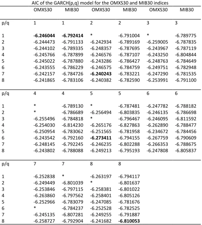
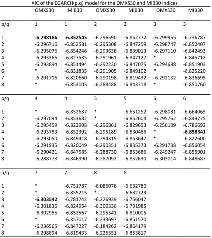
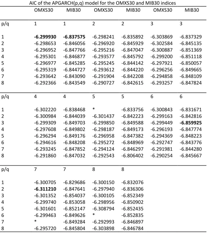
To test for higher orders of GARCH models the AIC criterion from EViews is used once again to find the best models. The results are shown in Table 5 through Table 8 in Appendix 2 through Appendix 5. For higher orders, GARCH(7,2), EGARCH(3,7), GJR-GARCH(4,8) and APGARCH(2,7) are the most suitable models for the OMXS30 index. For the MIB30 index, GARCH(8,8), EGARCH(4,6), GJR-GARCH(2,4) and APGARCH(3,6) are the most suitable models. An ARCH LM test was performed in order to ensure that there are no or few ARCH effects left in the residuals. The results of the ARCH LM test are shown in Table 9 in Appendix 6. All models passed the test. Thus, the models have been successful in removing any remaining ARCH effects in the data for both indices.

5.4

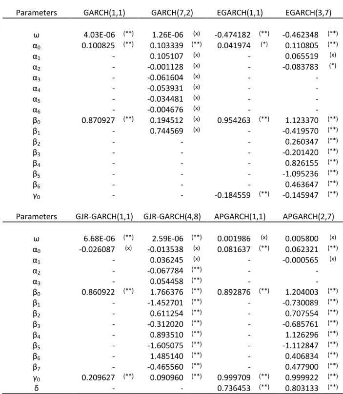
Estimated parameters

Table 10 and Table 11 in Appendix 7 shows the estimated parameters for the first order GARCH and the order higher than one that best fitted the data.

(24)

24

5.5

Forecast model evaluation

The one day ahead forecast for each model was evaluated with equation (24) as a proxy. An R2 statistic was used to rank the models. The regression parameters along with the p-value from the F-test are also presented. The results are shown in Table 2 and Table 3.

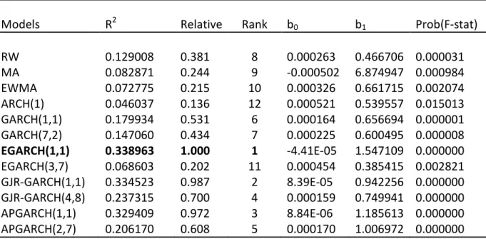
The R2 statistics are applied over the period 01/07/2008 to 30/12/2008. Model rankings are obtained by expressing the R2 statistics as a ratio relative to the worst performing model. The best model is marked in bold.

Table 2 – Model ranking from forecasting daily volatility for the OMXS30 index.

The R2 statistics are applied over the period 01/07/2008 to 30/12/2008. Model rankings are obtained by expressing the R2 statistics as a ratio relative to the worst performing model. The best model is marked in bold.

Table 3 – Model ranking from forecasting daily volatility for the MIB30 index. Model ranking from forecasting daily volatility for the OMXS30 index

Models R2 Relative Rank b0 b1 Prob(F-stat)

RW 0.129008 0.381 8 0.000263 0.466706 0.000031 MA 0.082871 0.244 9 -0.000502 6.874947 0.000984 EWMA 0.072775 0.215 10 0.000326 0.661715 0.002074 ARCH(1) 0.046037 0.136 12 0.000521 0.539557 0.015013 GARCH(1,1) 0.179934 0.531 6 0.000164 0.656694 0.000001 GARCH(7,2) 0.147060 0.434 7 0.000225 0.600495 0.000008 EGARCH(1,1) 0.338963 1.000 1 -4.41E-05 1.547109 0.000000 EGARCH(3,7) 0.068603 0.202 11 0.000454 0.385415 0.002821 GJR-GARCH(1,1) 0.334523 0.987 2 8.39E-05 0.942256 0.000000 GJR-GARCH(4,8) 0.237315 0.700 4 0.000159 0.749941 0.000000 APGARCH(1,1) 0.329409 0.972 3 8.84E-06 1.185613 0.000000 APGARCH(2,7) 0.206170 0.608 5 0.000170 1.006972 0.000000

Model ranking from forecasting daily volatility for the MIB30 index

Models R2 Relative Rank b0 b1 Prob(F-stat)

RW 0.205316 0.414 9 0.000190 0.299419 0.000000 MA 0.100968 0.204 11 -6.79E-05 4.593494 0.000272 EWMA 0.093425 0.188 12 0.000246 0.427981 0.000475 ARCH(1) 0.120536 0.243 10 0.000327 0.521438 0.000064 GARCH(1,1) 0.263071 0.531 7 0.000154 0.372716 0.000000 GARCH(8,8) 0.232090 0.468 8 0.000172 0.410482 0.000000 EGARCH(1,1) 0.495824 1.000 1 2.10E-06 1.303237 0.000000 EGARCH(4,6) 0.391830 0.790 4 0.000112 0.841082 0.000000 GJR-GARCH(1,1) 0.437723 0.883 2 0.000102 0.596572 0.000000 GJR-GARCH(2,4) 0.368879 0.744 6 0.000124 0.512730 0.000000 APGARCH(1,1) 0.413437 0.834 3 7.66E-05 0.660719 0.000000 APGARCH(3,6) 0.378037 0.762 5 0.000126 0.611588 0.000000

(25)

25 The results show that the EGARCH(1,1) model performed best during the forecast period for both indices. As the actual volatility is unobserved the range from equation (24) is plotted as a proxy against the forecasted volatilities to graphically show each models performance. The graphs are shown in Figure 11 through Figure 34 in Appendix 9 and Appendix 10.

6

Analysis and discussion

There is evidence in Figure 1 and Figure 2 of insignificant correlations for the indices returns. In Figure 7 and Figure 8 the autocorrelations in squared returns are significant and

persistent. The values found from the Ljung-Box Q-statistics and Engle’s Lagrange multiplier ARCH test further supports these findings. The Ljung-Box Q-statistics determines that the null hypothesis of no autocorrelation up to lag 10 cannot be rejected. There is also strong evidence of autoregressive conditional heteroskedasticity determined by the Lagrange multiplier ARCH test. Daily returns deviate from normality. This is shown in Figure 3 and Figure 4 and is also supported by the values of excess kurtosis and by the Jarque-Bera normality test. The Jarque-Bera null hypothesis is rejected at the 1% significance level. The indices are asymmetric or negatively skewed, which once again is supported by the values of excess kurtosis and by the values of skewness. The assumption of a zero mean cannot be rejected at the 1% significance level for both indices. The null hypothesis states that the return has a mean of zero. Figure 9 and Figure 10 also show evidence of volatility clustering. The augmented Dickey-Fuller test shows that there are no unit roots in return and squared return series for both indices. A time-series as daily data from a stock index is stationary if the mean and volatility do not depend on time. If a unit root exists it could lead to the non-existence of a stationary version of the volatility and lead to infinite volatility. These facts suggest that the GARCH models are preferred for more simple models. The GARCH models would also profit from having the innovation term from equation (7) to follow a distribution with fatter tails such as the student-t distribution. The models would then fit the data better. Although a better fit in the in-sample period would not necessarily mean a better forecast in the out-of-sample period. This can be seen from Table 2 and Table 4 where more or better information, in this case higher orders, doesn’t improve the forecasting.

The higher orders of GARCH models are not superior to the lower orders. In fact no higher order GARCH model outperforms the lower order models. This can also be seen in Appendix 6 where all or most ARCH effects have been removed by the models as the p-values for the test values reject the null hypothesis of existence of remaining ARCH effects. Thus, the volatility has been correctly specified for all GARCH models. Many GARCH models of higher orders have insignificant parameters. This simply means that if these parameters were zero they would not affect the outcome of the volatility from the model. Unfortunately many restrictions are also violated, i.e. ω, α or β parameters are negative. For the OMXS30 index the Maximum Likelihood Estimation does not converge on some occasions, which means that more information is necessary to add to the model specifications. A conclusion is therefore that these models are less attractive to use even though they outperform the more simple models. Interestingly the Random Walk model outperforms the MA, EWMA and ARCH(1) models for both indices. The RW model does however lack information from the range, which can be seen by the slope parameter b1 compared to the GARCH models.

GARCH models including the leverage effect seem to perform better. In particular the EGARCH(1,1) models performs best for both indices closely followed by the GJR-GARCH(1,1)

(26)

26 and APGARCH(1,1) specifications. As shown in Table 2 and Table 3 they are also unbiased, fairly efficient and include information about the range. If there was no information about the range the models lack representation of the underlying data on which the volatility is based.

7

Summary

This study has examined various models capability to predict volatility on the OMXS30 and MIB30 indices. The models, which were tested included the Random Walk, the Moving Average, the Exponential Weighted Moving Average, ARCH, GARCH, EGARCH, GJR-GARCH and APGARCH. The results suggest that GARCH models give better volatility forecasts than more simple models. Although the simple Random Walk model outperforms both ARCH, MA and EWMA models. In particular GARCH models, which includes the leverage effect

performs best for the period 31st of October 2003 to 30th of December 2008. Thus, the GARCH framework should be preferred to simpler volatility models when used for further risk management purposes.

8

Further research suggestions

Regression has been used to evaluate the volatility models in this study. Instead of a

regression approach one could use various error statistics to see if results differ. These error statistics could be Mean Error (ME), Mean Absolute Error (MAE), Root Mean Square Error (RMSE) or a Mean Absolute Percentage Error (MAPE) just to mention a few.

The study has focused on the assumption of normally distributed innovation terms. As seen in paragraph 5.2 this assumption does not reflect reality. It could therefore be interesting to evaluate the performance of the volatility models under the assumptions of a Student-t, Skewed Student-t, Gereralized Error Distribution or any other distribution of choice.

Only a one day forecast horizons has been investigated in this study. It could be interesting to see how the GARCH models perform under longer forecast horizons. More specifically the regime switching models or fractionally integrated models could be investigated as these handle longer forecast horizons better than the GARCH models presented in this study. For risk management purposes a volatility forecast using a volatility model is not really useful unless the results from the forecast are used to calculate risk measures. In particular such risk measures are the Value at Risk (VaR) or the Expected Shortfall (ES).

For further readings in the field of volatility forecasting it’s recommended to read the book Elements of Financial Risk Management by Christoffersen (2003). The Gloria Mundi (2009) website contains many interesting articles and research papers free to download. There is also a very interesting research paper written by Brailsford and Faff (1996), which evaluates many volatility forecasting techniques. Finally, the research papers mentioned in the

references, especially from Engle and Bollerslev are strongly recommended for further readings.

(27)

27

9

References

Baillie, R.T., Bollerslev, T. and Mikkelsen, H.O. (1996), ”Fractionally integrated generalized autoregressive conditional heteroskedasticity” Journal of Econometrics, 74, pp. 3-30. Bollerslev, T. (2008), ”Glossary to ARCH (GARCH)”, Duke University and NBER.

Brailsford, T.J. and Faff, R.W. (1996), “An evaluation of volatility forecasting techniques”, Journal of Banking & Finance, vol. 20, pp. 419-438.

Brooks, C. (2008), “Introductory Econometrics for Finance”, Cambridge University Press, 2nd

edition.

Engle, R.F. (1982), “Autoregressive Conditional Heteroscedasticity with Estimates of the Variance of UK Inflation”, Econometica 50/4, pp. 987-1007.

Engle, R.F. and Bollerslev, T. (1986), “Modeling the Persistence of Conditional Variances”, Econometric Review, 5, pp. 5-50.

Christoffersen, P. (2003), “Elements of Financial Risk Management”, Academic Press. Davidson, B. and Patel, R. (1994), “Forskningsmetodikens grunder”, Studentlitteratur, Lund. Ding, Zhuanxin; Granger, Clive, W.J. and Engle, R.F. (1993), “A long memory property of stock market returns and a new model”, Journal of Empirical Finance, vol. 1, pp. 83-106.

Glosten, Lawrence R., Jagannathan, Ravi and Runkle, David, E. (1993), ”On the Relation between the Expected Value and the Volatility of the Nominal Excess Return on Stocks”, The Journal of Finance, vol.48, pp. 1779-1801.

Gray, S. (1996), “Modeling the conditional distribution of interest rates as a regime- switching process", Journal of Financial Economics, 42, pp. 27-62.

Holme, I.M. and Solvang, B.K. (1994), “Forskningsmetodik”, Studentlitteratur, Lund. Hull, J.C. (2003), ”Options, Futures and Other Derivatives”, Prentice Hall, 5th edition.

Zakoian, J. (1994), ”Threshold heteroskedastic models”, Journal of Economic Dynamics and Control, vol. 18, pp. 931–955.

Jorion, P. (2001), “Value at Risk: The New Benchmark for Managing Financial Risk”, McGraw-Hill, 2nd edition.

Nelson, Daniel, B. (1991), “Conditional Heteroskedasticity in Asset Returns: A New Approach”, Econometrica, vol. 59, pp. 347-370.

(28)

28 Simons, K. (2000), “The use of Value at Risk by Institutional Investors”, New England

Economic Review, November-December.

BancWare Erisk. Case study Barings. Available (Online):

<http://www.erisk.com/Learning/CaseStudies/Barings.asp>(14th of November 2008) Mathworks (2007), “GARCH toolbox 2: User’s guide, version 2.3.2”. Available (Online): < http://www.mathworks.com>(29th of November 2008)

OECD Glossary of Statistical Terms. Available (Online):

<http://www.oecd.org/dataoecd/28/54/1890650.htm>(30th of November 2008) Quantitative Micro Software (2005), “EViews 5.1 Documentation”. Available (Online): <http://www.eviews.com>(18th of October 2008)

(29)

29

Appendix 1 – AIC results for the mean equation

Akaike Information Criterion (AIC) for the OMXS30 index

AR(p)/MA(q) MA(0) MA(1) MA(2) MA(3) MA(4) MA(5)

AR(0) -6.067246 -6.078126 -6.077659 -6.075990 -6.074794 -6.073125 AR(1) -6.078257 -6.076844 -6.075369 -6.073840 -6.072578 -6.070867 AR(2) -6.076171 -6.074796 -6.075844 -6.077211 -6.075700 -6.074056 AR(3) -6.074907 -6.073381 -6.076956 -6.075247 -6.073623 -6.075307 AR(4) -6.072923 -6.071382 -6.074451 -6.072751 -6.070695 -6.075694 AR(5) -6.071064 -6.069588 -6.076090 -6.074626 -6.072957 -6.071101

Akaike information criterion (AIC) for the MIB30 index

AR(p)/MA(q) MA(0) MA(1) MA(2) MA(3) MA(4) MA(5)

AR(0) -6.626344 -6.632771 -6.633854 -6.632189 -6.630920 -6.629237 AR(1) -6.634750 -6.633865 -6.633494 -6.631817 -6.630621 -6.628945 AR(2) -6.633979 -6.632423 -6.634178 -6.638326 -6.638469 -6.636832 AR(3) -6.632139 -6.630553 -6.638225 -6.636935 -6.635977 -6.634086 AR(4) -6.630064 -6.628892 -6.634569 -6.635135 -6.633817 -6.630871 AR(5) -6.629470 -6.628068 -6.631288 -6.633709 -6.633730 -6.646356

Table 4 – Akaike Information Criterion for the mean equation. The best fitted ARMA terms models are shown in bold.

(30)

30

Appendix 2 – AIC results of the GARCH(p,q) model

AIC of the GARCH(p,q) model for the OMXS30 and MIB30 indices

OMXS30 MIB30 OMXS30 MIB30 OMXS30 MIB30

p/q 1 1 2 2 3 3 1 -6.246044 -6.792414 * -6.791004 * -6.789775 2 -6.244473 -6.791133 -6.242934 -6.789169 -6.259005 -6.787835 3 -6.244102 -6.789335 -6.248357 -6.787695 -6.243967 -6.787119 4 -6.245766 -6.787899 -6.246576 -6.787107 -6.243250 -6.804844 5 -6.245022 -6.787880 -6.243286 -6.786427 -6.248763 -6.784649 6 -6.243555 -6.786229 -6.246575 -6.784759 -6.249751 -6.782948 7 -6.242157 -6.784726 -6.240243 -6.783221 -6.247290 -6.781535 8 -6.241865 -6.783106 -6.240382 -6.782590 -6.253991 -6.791100 p/q 4 4 5 5 6 6 1 * -6.789130 * -6.787481 -6.247782 -6.788182 2 * -6.786689 -6.256494 -6.803835 -6.246135 -6.786698 3 -6.255496 -6.784818 * -6.796467 -6.246095 -6.811592 4 -6.254030 -6.814230 -6.265176 -6.827863 -6.262890 -6.788477 5 -6.250954 -6.783062 -6.251565 -6.781958 -6.234672 -6.784456 6 -6.243542 -6.792160 -6.273411 -6.794155 -6.267759 -6.790609 7 -6.248145 -6.792245 -6.246235 -6.802288 -6.266353 -6.788675 8 -6.243802 -6.788088 -6.249213 -6.795193 -6.247808 -6.805837 p/q 7 7 8 8 1 -6.252838 * -6.263197 -6.794117 2 -6.249449 -6.801039 * -6.801637 3 -6.253846 -6.797115 -6.258381 -6.801022 4 -6.263860 -6.797562 -6.258401 -6.805126 5 -6.252966 -6.783079 -6.247085 -6.781676 6 * -6.784237 -6.252528 -6.782525 7 -6.245135 -6.807281 -6.249255 -6.791887 8 -6.258727 -6.792904 -6.241682 -6.810053

* MLE convergence not achieved after 500 iterations

Table 5 – AIC test for higher orders of GARCH for the OMXS30 and MIB30 indices. The lowest order and best fitted models are shown in bold.

(31)

31

Appendix 3 – AIC results of the EGARCH(p,q) model

AIC of the EGARCH(p,q) model for the OMXS30 and MIB30 indices

OMXS30 MIB30 OMXS30 MIB30 OMXS30 MIB30

p/q 1 1 2 2 3 3 1 -6.298186 -6.852545 -6.296590 -6.852772 -6.299955 -6.736787 2 -6.296716 -6.852581 -6.295308 -6.847259 -6.298747 -6.852407 3 -6.295076 -6.854246 -6.293638 -6.839013 -6.297110 -6.842493 4 -6.293366 -6.827535 -6.291961 -6.847127 * -6.845712 5 -6.293894 -6.851494 -6.292230 -6.847075 -6.294688 -6.851903 6 * -6.831835 -6.291905 -6.849102 * -6.825220 7 -6.291716 -6.820660 -6.290198 -6.819432 -6.292132 -6.836695 8 * -6.853003 -6.288488 -6.843718 * -6.850760 p/q 4 4 5 5 6 6 1 * -6.852687 * -6.651252 -6.298081 -6.664065 2 -6.297094 -6.853682 * -6.852604 -6.295762 -6.849775 3 -6.295459 -6.823908 -6.296861 -6.829653 -6.256109 -6.786692 4 -6.293783 -6.852392 -6.295189 -6.830466 * -6.858341 5 -6.293050 -6.849418 -6.294315 -6.853647 * -6.822600 6 -6.291935 -6.820049 -6.290351 -6.835373 -6.291738 -6.856054 7 -6.290421 -6.847585 -6.288730 -6.853686 -6.249247 -6.855901 8 -6.288778 -6.846990 -6.287092 -6.852630 -6.303014 -6.848687 p/q 7 7 8 8 1 * -6.751787 -6.086076 -6.632780 2 * -6.855215 * -6.632729 3 -6.303542 -6.781742 -6.226939 -6.756047 4 -6.301836 -6.824954 -6.300336 -6.791985 5 -6.302955 -6.852567 -6.295341 -6.810005 6 * -6.857017 -6.233697 -6.851570 7 -6.236565 -6.847227 -6.184262 -6.864179 8 -6.298894 -6.819433 -6.226551 -6.853817

Table 6 – AIC test for higher orders of EGARCH for the OMXS30 and MIB30 indices. The lowest order and best fitted models are shown in bold.

(32)

32

Appendix 4 – AIC results of the GJR-GARCH(p,q) model

AIC of the GJR-GARCH(p,q) model for the OMXS30 and MIB30 indices

OMXS30 MIB30 OMXS30 MIB30 OMXS30 MIB30

p/q 1 1 2 2 3 3 1 -6.281484 -6.844777 -6.279773 -6.835060 -6.282271 -6.845612 2 -6.281732 -6.848067 -6.280023 -6.843148 -6.281774 -6.845821 3 -6.280024 -6.844497 * -6.850016 -6.280073 -6.844705 4 -6.278313 -6.841984 -6.276607 -6.850415 -6.278819 -6.848659 5 -6.278550 -6.842627 * -6.841743 -6.277109 -6.849401 6 -6.281415 -6.842932 -6.278620 -6.841510 * -6.841182 7 -6.281059 -6.841063 -6.279347 -6.839938 -6.277523 -6.840130 8 -6.280803 -6.839663 -6.280071 -6.832955 -6.275583 -6.838491 p/q 4 4 5 5 6 6 1 -6.283589 -6.849222 -6.283074 -6.834240 -6.282263 -6.839498 2 * -6.854768 * -6.835863 -6.280688 -6.836842 3 * -6.849699 * -6.839446 -6.279248 -6.837106 4 -6.280181 -6.848535 -6.280535 -6.845865 -6.277186 -6.838983 5 -6.278734 -6.848088 -6.279150 -6.840388 -6.277635 -6.839667 6 -6.276844 -6.839486 -6.277837 -6.838951 -6.276127 -6.848830 7 -6.275923 -6.835292 -6.277293 -6.840998 * -6.833973 8 -6.273840 -6.833719 -6.274370 -6.835638 -6.271728 -6.832291 p/q 7 7 8 8 1 -6.289300 -6.841497 -6.288193 -6.838759 2 -6.287590 -6.838901 -6.286844 -6.835515 3 -6.285582 -6.850072 * -6.835595 4 -6.288928 -6.835968 -6.293611 -6.834135 5 -6.287526 -6.838838 -6.286274 -6.830561 6 -6.287758 -6.848080 -6.283972 -6.836846 7 -6.272454 -6.837972 -6.277711 -6.836473 8 -6.286343 -6.833256 -6.281771 -6.826143

Table 7 – AIC test for higher orders of GJR-GARCH for the OMXS30 and MIB30 indices. The lowest order and best fitted models are shown in bold.

(33)

33

Appendix 5 – AIC results of the APGARCH(p,q) model

AIC of the APGARCH(p,q) model for the OMXS30 and MIB30 indices

OMXS30 MIB30 OMXS30 MIB30 OMXS30 MIB30

p/q 1 1 2 2 3 3 1 -6.299930 -6.837575 -6.298241 -6.835892 -6.303869 -6.837329 2 -6.298653 -6.846056 -6.296920 -6.845929 -6.302584 -6.845135 3 -6.296952 -6.847766 -6.295216 -6.847047 -6.300887 -6.851369 4 -6.295301 -6.846877 -6.293577 -6.845792 -6.299200 -6.851118 5 -6.296977 -6.845285 -6.295245 -6.844142 -6.297921 -6.850057 6 -6.295319 -6.844727 -6.293612 -6.844220 -6.296256 -6.849665 7 -6.293642 -6.843090 -6.291904 -6.842208 -6.294858 -6.848109 8 -6.292366 -6.843549 -6.290727 -6.842615 -6.293257 -6.847824 p/q 4 4 5 5 6 6 1 -6.302220 -6.838468 * -6.833756 -6.300843 -6.831671 2 -6.300984 -6.844039 -6.301437 -6.842223 -6.299163 -6.842816 3 -6.299309 -6.849703 -6.299850 -6.849588 -6.299449 -6.859925 4 -6.297608 -6.849802 -6.298187 -6.849173 -6.296193 -6.847774 5 -6.296294 -6.849176 -6.296958 -6.847382 -6.294369 -6.848223 6 -6.294616 -6.848208 -6.295272 -6.848969 -6.292747 -6.843776 7 -6.293245 -6.847852 -6.294124 -6.846297 -6.291981 -6.844280 8 -6.291860 -6.847032 -6.292543 -6.806402 -6.290254 -6.845667 p/q 7 7 8 8 1 -6.300705 -6.829686 -6.300150 -6.832076 2 -6.311210 -6.847641 -6.297940 -6.836306 3 -6.301352 -6.854037 -6.300105 -6.852349 4 -6.299740 -6.853058 -6.298956 -6.850902 5 -6.301601 -6.852147 -6.308794 -6.852435 6 -6.299463 -6.849626 * -6.852835 7 * -6.849284 -6.292993 -6.846897 8 -6.295720 -6.845804 -6.303898 -6.846784

Table 8 – AIC test for higher orders of APGARCH for the OMXS30 and MIB30 indices. The lowest order and best fitted models are shown in bold.

(34)

34

Appendix 6 – ARCH LM test for the GARCH models

ARCH LM test of the GARCH(p,q) models for the OMXS30 and MIB30 indices

OMXS30 MIB30 OMXS30 MIB30

Statistics GARCH(1,1) GARCH(1,1) GARCH(7,2) GARCH(8,8)

F-statistic 0.041650 0.022618 0.006825 0.237868

(probability) 0.838324 0.880482 0.934173 0.625841

Obs*R-squared 0.041720 0.022656 0.006837 0.238224

(probability) 0.838154 0.880356 0.934103 0.625492

Statistics EGARCH(1,1) EGARCH(1,1) EGARCH(3,7) EGARCH(4,6)

F-statistic 0.122986 0.272039 0.075329 0.009579

(probability) 0.725882 0.602065 0.783779 0.922050

Obs*R-squared 0.123184 0.272439 0.075453 0.009595

(probability) 0.725607 0.601701 0.783556 0.921968

Statistics GJR-GARCH(1,1) GJR-GARCH(1,1) GJR-GARCH(4,8) GJR-GARCH(2,4)

F-statistic 1.022377 0.764937 0.215619 0.038064

(probability) 0.312166 0.381966 0.642485 0.845348

Obs*R-squared 1.023234 0.765740 0.215949 0.038128

(probability) 0.311753 0.381538 0.642144 0.845187

Statistics APGARCH(1,1) APGARCH(1,1) APGARCH(2,7) APGARCH(3,6)

F-statistic 0.064107 0.304500 0.453010 3.144734

(probability) 0.800163 0.581180 0.501042 0.076431

Obs*R

Volatility forecasting using the GARCH framework on the OMXS30 and MIB30 stock indices