Long-term correlation tracking using multi-layer hybrid features in sparse and dense environments

Long-term Correlation Tracking using Multi-layer

Hybrid Features in Sparse and Dense Environments

Nathanael L. Baisaa,∗, Deepayan Bhowmikb, Andrew Wallacea a_{School of Engineering and Physical Sciences, Heriot Watt University, Edinburgh, United}

Kingdom

b_{Department of Computing, Sheffield Hallam University, Sheffield, United Kingdom}

Abstract

Tracking a target of interest in both sparse and crowded environments is a chal-lenging problem, not yet successfully addressed in the literature. In this paper, we propose a new long-term visual tracking algorithm, learning discriminative correlation filters and using an online classifier, to track a target of interest in both sparse and crowded video sequences. First, we learn a translation corre-lation filter using a multi-layer hybrid of convolutional neural networks (CNN) and traditional hand-crafted features. Second, we include a re-detection module for overcoming tracking failures due to long-term occlusions using online SVM and Gaussian mixture probability hypothesis density (GM-PHD) filter. Finally, we learn a scale correlation filter for estimating the scale of a target by con-structing a target pyramid around the estimated or re-detected position using the HOG features. We carry out extensive experiments on both sparse and dense data sets which show that our method significantly outperforms state-of-the-art methods.

Keywords: Visual tracking, Correlation filter, CNN features, Hybrid features, Online learning, GM-PHD filter

∗_{Corresponding author}

1. Introduction

Visual target tracking is one of the most important and active research areas in computer vision with a wide range of applications like surveillance, robotics and human-computer interaction (HCI). Although it has been studied exten-sively during past decades as recently surveyed in [1][2], object tracking is still 5

a difficult problem due to many challenges that cause significant appearance changes of targets such as varying illumination, occlusion, pose variations, de-formation, abrupt motion, background clutter, and high target densities (in crowded environments). Robust representation of target appearance is impor-tant to overcome these challenges.

10

Recently, convolutional neural network (CNN) features have demonstrated out-standing results on various recognition tasks [3, 4]. Motivated by this, a few deep learning based trackers [5, 6] have been developed. In addition, discrimi-native correlation filter-based trackers have achieved state-of-the-art results as surveyed in [7] in terms of both efficiency and robustness due to three reasons. 15

First, efficient correlation operations are performed by replacing exhausted cir-cular convolutions with element-wise multiplications in the frequency domain which can be computed using the fast Fourier transform (FFT) with very high speed. Second, thousands of negative samples around the target’s environment can be efficiently incorporated through circular-shifting with the help of a circu-20

lant matrix. Third, training samples are regressed to soft labels of a Gaussian function (Gaussian-weighted labels) instead of binary labels alleviating sam-pling ambiguity. In fact, regression with class labels can be seen as classifi-cation. However, correlation filter-based trackers are susceptible to long-term occlusions.

25

In addition, the Gaussian mixture probability hypothesis density (GM-PHD) filter [8] has an in-built capability of removing clutter while filtering targets with very efficient speed without the need for explicit data association. Though this filter is designed for multi-target filtering, it is even preferable for single target filtering in scenes with challenging background clutter as well as clutter 30

that comes from other targets not of current concern. This filtering approach is flexible, for instance, it has been extended for multiple targets of different types in [9][10].

In this work, we mainly focus on long-term tracking of a target of interest in sparse as well as crowded environments where the unknown target is initialized 35

by a bounding box and then tracked in subsequent frames. Without making any constraint on the video scene, we develop a novel long-term online tracking algorithm that can close the research gap between sparse and crowded scenes tracking problems using the advantages of the correlation filters, a hybrid of multi-layer CNN and hand-crafted features, an incremental (online) support 40

vector machine (SVM) classifier and a Gaussian mixture probability hypothesis density (GM-PHD) filter. To the best of our knowledge, nobody has adopted this approach.

The main contributions of this paper are as follows:

1. We integrate a hybrid of multi-layer CNN and traditional hand-crafted fea-45

tures for learning a translation correlation filter for estimating the target position in the next frame by extending a ridge regression for multi-layer features.

2. We include a re-detection module to re-initialize the tracker in case of tracking failures due to long-term occlusions by learning an incremental 50

SVM from the most confident frames using hand-crafted features to gen-erate high score detection proposals.

3. We incorporate a GM-PHD filter to temporally filter detection proposals generated from the learned online SVM to find the detection proposal with the maximum weight as the target position estimate by removing 55

the other detection proposals as clutter.

4. We learn a scale correlation filter by constructing a target pyramid at the estimated or re-detected position using HOG features to estimate the scale of the detected target.

We presented a preliminary idea of this work in [11]. In this work, we make more 60

elaborate descriptions of our algorithm. Besides, we include a scale estimation at the estimated target position as well as an extended experiment on a large-scale online object tracking benchmark (OOTB) in addition to the PETS 2009 data sets.

The rest of this paper is organized as follows. In section 2, related work is 65

discussed. An overview of our algorithm and the proposed algorithm in detail are described in sections 3 and 4, respectively. In section 5, the implementation details with parameter settings is briefly discussed. The experimental results are analyzed and compared in section 6. The main conclusions and suggestions for future work are summarized in section 7.

70

2. Related Work

Various visual tracking algorithms have been proposed over the past decades to cope with tracking challenges, and they can be categorized into two types depending on the learning strategies: generative and discriminative methods. Generative methods describe the target appearances using generative models 75

and search for target regions that fit the models i.e. search for the best-matching windows (patches). Various generative target appearance modelling algorithms have been proposed such as online density estimation [12], sparse representation [13, 14], and incremental subspace learning [15]. On the other hand,discriminative methods build a model that distinguishes the target from 80

the background. These algorithms typically learn classifiers based on online boosting [16], multiple instance learning [17], P-N learning [18], transfer learn-ing [19], structured output SVMs [20] and combinlearn-ing multiple classifiers with different learning rates [21]. Background information is important for effective tracking as explored in [22][23] which means that more competing approaches 85

are discriminative methods [24] though hybrid generative and discriminative models can also be used [25][26]. However, sampling ambiguity is one of the big problems in discriminative tracking methods which results in drifting. Re-cently, correlation filters [27, 28, 29] have been introduced for online target

tracking that can alleviate this sampling ambiguity. Previously, the large train-90

ing data required to train correlation filters prevented them from application to online visual tracking though correlation filters are effective for localization tasks. However, recently all the circular-shifted versions of input features have been considered with the help of a circulant matrix producing a large number training samples [27, 28].

95

There are many strong sides of correlation methods such as inherent paral-lelism, shift (translation) invariance, noise robustness, and high discrimination ability [30]. Both digital and optical correlators are discussed in detail in [31] though more emphasis is given to optical correlators. Performance optimization of the correlation filters by pre-processing the input target image was introduced 100

in [32]. Recent research trends of correlation filters for various applications with more emphasis on face recognition (and object tracking) is given in [30]. Due to the effectiveness of the correlation methods, they have been successfully applied to many domains such as swimmer tracking [33], pose invariant face recogni-tion [34], road sign identificarecogni-tion for advanced driver assistance [35], etc. Some 105

types of correlation filters are sensitive to challenges such as rotation, illumi-nation changes, occlusion, etc. For instance, the Phase-Only Filter (POF) is sensitive to changes in rotation, illumination changes, occlusion, scale and noise contained in targets of interest [32] though it can give very narrow correlation peaks (good localization); a pre-processing step was used to make it invariant 110

to illumination in [34]. Recent correlation filters such as KCF [28] are more suitable for online tracking by generating a large number of training samples from input features using a circulant matrix and are more robust to the tracking challenges such as rotation, illumination changes, partial occlusion, deformation, fast motion, etc (as shown on its results section in [28]) than its previous coun-115

terparts [30]. Using CNN features has even improved the online tracking results as shown in [36] against these tracking challenges, however, log-term occlusion is still a problem in correlation filter-based tracking approaches.

There are three tracking scenarios that are important to consider: short-term tracking, long-term tracking, and tracking in a crowded scene. If objects are 120

visible over the whole course of the sequences, short-term model-free tracking algorithms are sufficient to track a single object without applying a pre-trained model of target appearance. There are many short-term tracking algorithms developed in the literature [1][7] such as online density estimation [12], context-learning [37], scale estimation [29], and using features from multiple CNN lay-125

ers [36, 38]. However, these short-term tracking algorithms can not re-initialize the trackers once they fail due to long-term occlusions and confusions from background clutter.

Long-term tracking algorithms are important in video streams that are of in-definite length and have long-term occlusions. A Tracking-Learning-Detection 130

(TLD) algorithm has been developed in [18] which explicitly decomposes the long-term tracking task into tracking, learning and detection. In this case, the tracker tracks the target from frame to frame and provides training data for the detector which re-initializes the tracker when it fails. The learning component estimates the detector’s errors and then updates it for correction in the fu-135

ture. This algorithm works well in very sparse videos (video sequences with few targets) but is sensitive to background clutter. Long-term correlation tracking (LCT), developed in [39], learns three different discriminative correlation filters: translation, appearance and scale correlation filters using hand-crafted features. Even though it includes a re-detection module by learning the random ferns 140

classifier online for re-initializing a tracker in case of tracking failures, it is not robust to long-term occlusions and background clutter. Multi-domain network (MDNet) [40] pre-trains a CNN network composed of shared layers and multiple domain-specific layers using a large set of videos to get generic target represen-tations in the shared layers. This proposed network has separate branches of 145

domain-specific layers for binary classification to identify the target in each do-main. However, when applied to fundamentally different videos other than the related videos on which it was trained, it gives poorer results.

Tracking of a target in a crowded scene is very challenging due to long-term occlusion, many targets with appearance variation and high clutter. Person 150

problem by combining crowd density estimation and localization of individual person in [41]. Although this approach does not require manual initialization, it has low performance for tracking a generic target of interest as it was mainly developed for tracking human heads. The method developed in [42] trained 155

Hidden Markov Models (HMMs) on motion patterns within a scene to capture spatial and temporal variations of motion in the crowd which is used for track-ing individuals. However, this approach is limited to a crowd with structured pattern i.e. it needs some prior knowledge about the scene. The algorithm developed in [43] used visual information (prominence) and spatial context (in-160

fluence from neighbours) to develop online tracking in crowded scene without using any prior knowledge about the scene, unlike the method in [42] which uses some training data from the past as well as the future. This algorithm performs well in highly crowded scenes but has low performance in a less crowded scenes as influence from neighbours (spatial context) decreases.

165

In conclusion, although there are many effective algorithms that handle ap-pearance variation, occlusion and high clutter in short and long-term video sequences, no single approach is wholly effective in all scenarios. Our proposed tracking algorithm tracks a target of interest in both sparse and dense environ-ments without using any constraint from the video scene using correlation filters, 170

sophisticated features and re-detection scheme particularly robust to sparse as well as highly occluded and cluttered dense scenes.

3. Overview of Our Algorithm

We develop a novel long-term online tracking algorithm that can be applied to both sparse and dense environments by learning correlation filters using a hybrid 175

of multi-layer CNN and hand-crafted features as well as including a re-detection module using an incremental SVM and GM-PHD filter.

Accordingly, to develop an online long-term tracking algorithm robust to ap-pearance variations in both sparse and crowded scenes, we learn two different correlation filters: a translation correlation filter (wt) and a scale correlation

ter (ws). A translation correlation filter is learned using a hybrid of multi-layer

CNN features from VGG-Net [4] and robust traditional hand-crafted features. For the CNN part, we combine features from both a lower convolutional layer which retains more spatial details for precise localization and a higher con-volutional layer which encodes semantic information for handling appearance 185

variations. This makes layer 1, layer 2 and layer 3 in multi-layer features with multiple channels (512, 512 and 256 dimensions) in each layer, respectively. Since the spatial resolution of the extracted features gradually reduces with the increase of the depth of CNN layers due to pooling operators, it is crucial to resize each feature map to a fixed size using bilinear interpolation.

190

For the traditional features part, we use a histogram of oriented gradients (HOG), in particular Felzenszwalb’s variant [44] and color-naming [45] features for capturing image gradients and color information, respectively. These in-tegrated traditional features were used for object detection in [46][47] giving promising results. Color-naming is the linguistic color label assigned by hu-195

man to describe the color, hence, the mapping method in [45] is employed to convert the RGB space into the color name space which is an 11 dimensional color representation providing the perception of a target color. By aligning the feature size of the HOG variant with 31 dimensions and color-naming with 11 dimensions, they are integrated to make 42 dimensional features which make a 200

4th layer in our hybrid multi-layer features.

For scale estimation, we learn a scale correlation filter using only HOG features, in particular Felzenszwalb’s variant [44]. Besides, we incorporate a re-detection module by learning an incremental SVM from the most confident frames deter-mined by maximal value of correlation response map using HOG, LUV color 205

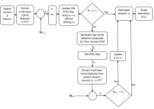
and normalized gradient magnitude features for generating high-score detection proposals which are filtered using the GM-PHD filter to re-acquire the target in case of tracking failures. The flowchart of our method is given in Fig. 1 and the outline of our proposed algorithm is given in Algorithm 1.

Figure 1: The flowchart of the proposed algorithm. It consists of three main parts: translation estimation, re-detection and scale estimation. Given a search window, we extract multi-layer hybrid features (in the frequency domain) and then estimate target position (xk) using a translation correlation filter (wt). This estimated position (xk)

is used as a measurement (zk) for updating the GM-PHD filter without refiningxk,

just to update its weight for later use during re-detection. Re-detection is activated if the maximum of the response map (Rm) becomes below the pre-defined threshold

(Trd). Then, we generate high score detection proposals (Zk)which are filtered by the

GM-PHD filter to estimate the detection with maximum weight as target position (xrk) removing the others as clutter. If the response map aroundxrk(Rmd) is greater

thanTrd, the target position xk is updated by the re-detected positionxrk. Finally,

we estimate the scale of the target by constructing a target pyramid at the estimated position and use the scale correlation filter (ws) to find the scale at which the maximum

response map is obtained. Note that in frame 1, we only train correlation filters and the SVM classifier using the initialized target; no detection is performed.

4. Proposed Algorithm

210

This section describes our proposed tracking algorithm which has four distinct functional parts: a) correlation filters formulated for multi-layer hybrid features, b) an online SVM detector developed for generating high score detection pro-posals, c) a GM-PHD filter for finding the detection proposal with maximum weight to re-initialize the tracker in case of tracking failures by removing the 215

other detection proposals as clutter, and d) a scale estimation method for es-timating the scale of a target by constructing image pyramid at the estimated target position.

4.1. Correlation Filters for Multi-layer Features

To track a target using correlation filters, the appearance of the target should be 220

modeled using a correlation filterw which can be trained on feature vectorxof sizeM×N×Dextracted from an image patch where M, N, and D indicates the width, height and number of channels, respectively. This feature vectorxcan be extracted from multiple layers, for example in the case of CNN features and/or traditional hand-crafted features, therefore, we denote it as x(l) _{to designate}

225

from which layerlit is extracted. All the circular shifts ofx(l)_{along theM and}

N dimensions are considered as training examples where each circularly shifted samplex(l)m,n, m∈ {0,1, ..., M−1}, n∈ {0,1, ..., N−1}has a Gaussian function

labely(l)(m, n) given by

y(l)(m, n) =e−(m

−M/2)2 +(n−N/2)2

2σ2 _{, (1)}

whereσis the kernel width. Hence,y(l)_{(m, n) is a soft label rather than a binary}

230

label. To learn the correlation filterw(l)_{for layer l with the same size as x}(l)_,

we extend a ridge regression [48][49], developed for a single-layer feature vector, to be used for multi-layer hybrid features with layerlas

min w(l)

X

m,n

where Φ denotes the mapping to a kernel space andλ is a regularization pa-rameter (λ≥0). The solutionw(l) can be expressed as

235

w(l)=X

m,n

a(l)(m, n)Φ(x(l)_m,n), (3)

This alternative representation makes the dual space a(l) _{the variable under}

optimization instead of the primal spacew(l)_.

Training phase: The training phase is performed in the Fourier domain using

the fast Fourier transform (FFT) to compute the coefficientA(l) as

A(l)=F(a(l)) = F(y

(l)₎ F Φ(x(l)_).Φ(x(l)₎

+λ, (4)

whereF denotes the FFT operator. 240

Detection phase: The detection phase is performed on the new frame given

an image patch (search window) which is used as a temporal context i.e. the search window is larger than the target to provide some context. If feature vectorz(l)_{of sizeM ×N×D is extracted from this image patch, the response}

map (r(l)) is computed as

r(l)=F−1 A˜(l) F(Φ(z(l)).Φ(˜x(l))), (5)

where ˜A(l) _{and ˜x}(l) _=F−1_{( ˜X}(l)_{) denote the learned target appearance model}

for layerl, operatoris the Hadamard (element-wise) product, andF−1is the inverse FFT. Now, the response maps of all layers are summed according to their weightγ(l) element-wise as

r(m, n) =X

l

γ(l)r(l)(m, n), (6)

The new target position is estimated by finding the maximum value ofr(m, n) as

( ˆm,nˆ) = argmax

m,n

r(m, n), (7)

Model update: The model is updated by training a new model at the new

245

space coefficients A(l)_k and the base data template X(l)_k = F(x(l)_k ) with those from the previous frame to make the tracker more adaptive to target appearance variations.

˜

X(l)_k = (1−η) ˜X(l)_k−1+ηX(l)_k , (8a)

˜

A(l)_k = (1−η) ˜A(l)_k−1+ηA(l)_k , (8b)

wherekis the index of the current frame, andη is the learning rate. 250

The mappings to the kernel space (Φ) used in Eq. (4) and Eq. (5) can be ex-pressed using a kernel function asK(x(l)_i ,x(l)_j ) = Φ(x(l)_i ).Φ(x(l)_j ) = Φ(x(l)_i )TΦ(x(l)_j ). If the computation is performed in the frequency domain, the normal transpose should be replaced by the Hermitian transpose i.e. Φ(X(l)_i )H _{= (Φ(X}(l)

i )∗) T

where the star (∗) denotes the complex conjugate. 255

Thus, for a linear kernel,

K(x(l)_i ,x(l)_j ) = (x(l)_i )Tx(l)_j =F−1(X

d

(X(l)_i,d)∗X(l)_j,d), (9)

whereX(l)_i =F(x(l)_i ). and for a Gaussian kernel,

K(x(l)_i ,x(l)_j ) = Φ(x(l)_i )T_Φ(x(l) j ) = exp − |x(_il)−x(_jl)|2 σ2 = exp − 1 σ2 kx (l) i k2+kx (l) j k2− F−1( P d(X (l) i,d) ∗_X(l) j,d) , (10)

This formulation is generic for multiple channel features from multiple layers as in the case of our multi-layer hybrid features, i.e. whereX(l)_i,d, d∈ {1, ..., D}, l∈ {1, ..., L}. This is an extended version of the one given in [28] that takes into account features from multiple layers. The linearity of the FFT allows us to 260

simply sum the individual dot-products for each channeld∈ {1, ..., D} in each layerl∈ {1, ..., L}.

4.2. Online Detector

We include a re-detection module,Dr, to generate high score detection

propos-als in case of tracking failures due to long-term occlusions. Instead of using a 265

correlation filter to scan across the entire frame which is computationally expen-sive and less efficient, we learn an incremental (online) SVM [50] by generating a set of samples in the search window around the estimated target position from the most confident frames, and scan through the window when the re-detection is activated to generate high-score detection proposals. These most confident 270

frames are determined by the maximum translation correlation response in the current frame i.e. if the maximum correlation response of an image patch is above the trained detector threshold (Ttd), we generate samples around this

image patch and train the detector. This detector is activated to generate high score detection proposals if the maximum of the correlation response becomes 275

below the activated re-detection threshold (Trd). We use HOG (particularly

Felzenszwalb’s variant [44]), LUV color and normalized gradient magnitude fea-tures to train this online SVM classifier. We use different visual feafea-tures for computational feasibility from the ones we use for learning the translation cor-relation filter since we can select the feature representation for each module 280

independently [29, 39].

We want to update a weight vector w of the SVM provided a set of samples with associated labels,{(´xi,y´i)}, obtained from the current results. The label

´

yi of a new example ´xi is given by

´ yi=      +1, ifIOU(´xi,x¨t)≥δp −1, ifIOU(´xi,x¨t)< δn (11)

where IOU(.) is the intersection over union (overlap ratio) of a new example 285

´

xi and the estimated target bounding box in the current most confident frame

¨

xt. The samples with the bounding box overlap ratios between the thresholds

δn andδp are excluded from the training set for avoiding the drift problem.

SVM classifiers of the form f(x) = w.Φ(x) +b are learned from the data

{(xi,yi)∈ <m× {−1,+1}∀i∈ {1, ..., N}}by minimizing 290 min w,b,ξ 1 2||w|| 2_+C N X i=1 ξp_i (12)

forp∈ {1,2} subject to the constraints

yi(w.Φ(xi) +b)≥1−ξi, ξi≥0∀i∈ {1, ..., N}. (13)

Hinge loss (p= 1) is preferred due to its improved robustness to outliers over the quadratic loss (p= 2). Thus, the offline SVM learns a weight vectorw = (w1, w2, ...., wN)T by solving this quadratic convex optimization problem (QP)

which can be expressed in its dual form as

min 0≤ai≤C W = 1 2 N X i,j=1 aiQijaj− N X i=1 ai+b N X i=1 yiai, (14)

where {ai} are Lagrange multipliers, b is bias, C is regularization parameter,

295

andQij =yiyjK(xi,xj). The kernel function K(xi,xj) = Φ(xi).Φ(xj) is used to implicitly map into a higher dimensional feature space and compute the dot product. It is not straightforward for conventional QP solvers to handle the optimization problem in Eq. (14) for online tracking tasks as the training data are provided sequentially, not at once. Incremental SVM [50] is tailored 300

for such cases which retains Karush-Kuhn-Tucker (KKT) conditions on all the existing examples while updating the model with a new example so that the exact solution at each increment of dataset can be guaranteed. KKT conditions are the first-order necessary conditions for the optimal unique solution of dual parameters{a, b} which minimizes Eq. (14) and are given by

305 ∂W ∂ai = N X j=1 Qijaj+yib−1            >0,ifai= 0 = 0,if 0≤ai≤C <0,ifai=C, (15) ∂W ∂b = N X j=1 yjaj= 0, (16)

Based on the partial derivativemi = ∂W_∂a

i which is related to the margin of the i-th example, each training example can be categorized into three: S1 support

(mi <0), and the remaining Rreserve vectors (non-support vectors). During

incremental learning, new examples withmi≤0 eventually become margin (S1)

310

or error (S2) support vectors. However, the remaining new training examples

become reserve vectors as they do not enter the solution so that the Lagrangian multipliers (ai) are estimated while retaining the KKT conditions. Given the

updated Lagrangian multipliers, the weight vectorw is given by

w= X

i∈S1∪S2

aiyiΦ(xi), (17)

It is important to keep only a fixed number of support vectors with the smallest 315

margins for efficiency during online tracking.

Thus, using the trained incremental SVM, we generate high score detections as detection proposals during the re-detection stage. These are filtered using the GM-PHD filter to find the best possible detection that can re-initialize the tracker.

320

4.3. Temporal Filtering using the GM-PHD Filter

Once we generate high score detection proposals using the learned online SVM classifier during the re-detection stage, we need to find the most probable de-tection proposal for the target state (position) estimate by finding the dede-tection proposal with the maximum weight using the GM-PHD filter [8]. Though the 325

GM-PHD filter is designed for multi-target filtering with the assumptions of a linear Gaussian system, in our problem (re-detecting a target in cluttered scene), it is used for removing clutter that comes from background scene and other targets not of interest as it is equipped with such a capability. Besides, it provides motion information for the tracking algorithm. More importantly, 330

using the GM-PHD filter to find the detection with the maximum weight from the generated high score detection proposals is more robust than relying only on the maximum score of the classifier.

The detected position of the target in each frame is filtered using the GM-PHD filter, but without re-fining the position states until the re-detection module is 335

activated. This updates the weight of the GM-PHD filter corresponding to a target of interest giving sufficient prior information to be picked up during the detection stage among candidate high score detection proposals. If the re-detection module is activated (correlation response of the target becomes below a pre-defined threshold), we generate high score detection proposals (in this case 340

5) from the trained SVM classifier which are then filtered using the GM-PHD filter. The Gaussian component with the maximum weight is selected as the position estimate, and if the correlation response of this estimated position is greater than the pre-defined threshold, the estimated position of the target is re-fined.

345

The GM-PHD filter has two steps: prediction and update. Before stating these two steps, certain assumptions are needed: 1) each target follows a linear Gaus-sian model:

y_k|k−1(x|ζ) =N(x;Fk−1ζ, Qk−1) (18)

fk(z|x) =N(z;Hkx, Rk) (19)

where N(.;m, P) denotes a Gaussian density with mean m and covarianceP; Fk−1 and Hk are the state transition and measurement matrices, respectively.

350

Qk−1 and Rk are the covariance matrices of the process and the measurement

noises, respectively. 2) A current measurement driven birth intensity inspired by but not identical to [51] is introduced at each time step, removing the need for the prior knowledge (specification of birth intensities) or a random model, with a non-informative zero initial velocity. The intensity of the spontaneous 355

birth RFS is a Gaussian mixture of the form

γk(x) = Vγ,k X

v=1

w(v)_γ,kN(x;m(v)_γ,k, P_γ,k(v)) (20)

where Vγ,k is the number of birth Gaussian components, w (v)

γ,k is the weight

and zero initial velocity used as mean, andP_γ,k(v)is birth covariance for Gaussian componentv. In our case,Vγ,k equals to 1 unless in re-detection stage at which

360

it becomes 5 as we generate 5 high score detection proposals to be filtered. 3) The survival and detection probabilities are independent of the target state: ps,k(xk) =ps,kandpD,k(xk) =pD,k.

Prediction: It is assumed that the posterior intensity at timek−1 is a Gaussian

mixture of the form 365 Dk−1(x) = Vk−1 X v=1 w_k−1(v) N(x;m(v)_k−1, P_k−1(v)), (21)

whereVk−1 is the number of Gaussian components ofDk−1(x) and it equals to

the number of Gaussian components after pruning and merging at the previous iteration. Under these assumptions, the predicted intensity at time kis given by Dk|k−1(x) =DS,k|k(x) +γk(x), (22) where 370 DS,k|k−1(x) = ps,kP Vk−1 v=1 w (v) k−1N(x;m (v) S,k|k−1, P (v) S,k|k−1), m(v)_S,k|k−1=Fk−1m(v)_k−1, P_S,k|k−1(v) =Qk−1+Fk−1Pk−1(v)F T k−1,

whereγk(x) is given by Eq. (20).

SinceDS,k|k−1(x) andγk(x) are Gaussian mixtures,Dk|k−1(x) can be expressed

as a Gaussian mixture of the form

Dk|k−1(x) = Vk|k−1

X

v=1

where w(v)_k|k−1 is the weight accompanying the predicted Gaussian component v, and V_k|k−1 is the number of predicted Gaussian components and it equals 375

to the number of born targets (1 unless in case of re-detection at which it is 5) and the number of persistent components which are actually the number of Gaussian components after pruning and merging at the previous iteration.

Update: The posterior intensity (updated PHD) at timek is also a Gaussian

mixture and is given by

Dk|k(x) = (1−pD,k)Dk|k−1(x) + X z∈Zk DD,k(x;z), ₍₂₄₎ where DD,k(x;z) = Vk|k−1 X v=1 w_k(v)(z)N(x;m(v)_k|k(z), P_k|k(v)), w(v)_k (z) = pD,kw (v) k|k−1q (v) k (z) csk(z) +pD,k PVk|k−1 l=1 w (l) k|k−1q (l) k (z) , q_k(v)(z) =N(z;Hkm (v) k|k−1, Rk+HkP (v) k|k−1H T k), m(v)_k|k(z) =m(v)_k|k−1+K_k(v)(z−Hkm (v) k|k−1), P_k|k(v)= [I−K_k(v)Hk]P (v) k|k−1, K_k(v)=P_k|k−1(v) H_kT[HkP (v) k|k−1H T k +Rk]−1,

The clutter intensity due to the scene,csk(z), in Eq. (24) is given by

wherec(.) is the uniform density over the surveillance region A, andλc is the

average number of clutter returns per unit volume i.e. λt =λcA. We set the

380

clutter rate or false positive per image (fppi)λt= 4 in our experiment.

After update, weak Gaussian components with weight w(v)_k < T = 10−5 _are

pruned, and Gaussian components with Mahalanobis distance less thanU = 4 pixels from each other are merged. These pruned and merged Gaussian com-ponents are predicted as existing targets in the next iteration. Finally, the 385

Gaussian component of the posterior intensity with mean corresponding to the maximum weight is selected as a target state (position) estimate when the re-detection module is activated.

4.4. Scale Estimation

At the new estimated target position (or re-fined target position after re-detection 390

in case of tracking failure), we construct an image pyramid for estimating its scale. Given a target size ofP×Qin a test frame, we generateSnumber of scale levels at the new estimated position i.e. for eachn∈ {b−S−1₂ c,b−S−3₂ c, ...,bS−1₂ c}, we extract an image patchIs of size sP ×sQ centered at the new estimated

target position, where scales=an andais the scale factor between the gener-395

ated image pyramids. We uniformly resize all the generated image pyramids to P×Qagain unlike [29], and extracted HOG features particularly Felzenszwalb’s variant [44] to construct the scale feature pyramid. Then, the optimal scale ˆs of a target at the estimated new position can be obtained by computing the correlation response maps ˆrsof the scale correlation filterwstoIsand find the

400

scale at which the maximum response map can be obtained as

ˆ s= argmax s ˆ rs , (26)

The scale correlation filter is updated using the new training sample at the estimated scaleIsˆby Eq. (8).

Algorithm 1Proposed tracking algorithm

1: Input: ImageIk, previous target positionxk−1and scalesk−1, previous correlation filters

w(_t,kl)₋₁andws,k−1, previous SVM detectorDr

2: Output: Estimated target positionxk= (xk, yk) and scalesk, updated correlation filters w_t,k(l) andws,k, updated SVM detectorDr

3: repeat

4: Crop out the searching window in frame k according to (xk−1, yk−1) andsk−1, and then

extract multi-layer hybrid features and resize them to a fixed size; // Translation estimation

5: for eachlayer ldo

6: compute response mapr(l)_usingw(l)

t,k−1and Eq. (5);

7: end for

8: Sum up the response maps of all layers element-wise according to their weightγ(l) to get

r(m, n) using Eq. (6);

9: Estimate the new target position (xk, yk) by finding the maximum response ofr(m, n)

using Eq. (7);

// Apply GM-PHD filter

10: Update GM-PHD filter using the estimated target position (xk, yk) as measurement but

without re-fining it, just to update weight of GM-PHD filter for later use; // Target re-detection

11: ifmax r(m, n)

< Trdthen

12: Use the detectorDrto generate detection proposalsZkfrom high scores of incremental

SVM;

// Filtering using GM-PHD filter

13: Filter the generated candidate detectionsZkusing GM-PHD filter and select the

detection with maximum weight as a re-detected target position (xrk, yrk). Then crop

out the searching window at this re-detected position and compute its response map using Eq. (5) and Eq. (6), and call itrrd(m, n);

14: ifmax rrd(m, n)

> Trdthen

15: (xk, yk) = (xrk, yrk) i.e. re-fine by the re-detected position;

16: end if 17: end if

// Scale estimation

18: Construct target image pyramid around (xk, yk) and extract HOG features (resized to same

size), and then compute the response maps ˆrsusingws,k−1and Eq. (5), and then estimate

its scaleskusing Eq. (26);

// Translation correlation model update

19: Crop out new patch centered at (xk, yk) and extract multi-layer hybrid features and resize

them to a fixed size; 20: for eachlayer ldo

21: Update translation correlation filterw(_t,kl) using Eq. (8); 22: end for

// Scale correlation model update

23: Crop out new patch centered at (xk, yk) with estimated scaleskand extract HOG features

and then update correlation filterws,kusing Eq. (8);

// Detector update

24: ifmax r(m, n)

≥Ttdthen

25: Generate positive and negative samples around (xk, yk) and then extract HOG, LUV

5. Implementation Details

The main steps of our proposed algorithm are presented in Algorithm 1. More 405

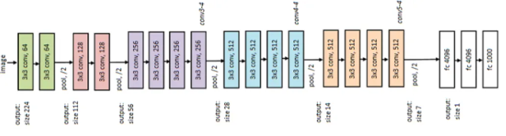
implementation details with parameter settings are given as follows. For learning the translation correlation filter, we extract features from VGG-Net [4], shown in Fig. 2, trained on a large amount of object recognition data set (ImageNet) [52] by first removing fully-connected layers. Particularly, we use outputs ofconv 3-4,conv4-4 and conv5-4 convolutional layers as features (l ∈ {1,2,3} and d∈

410

{1, ..., D}), i.e. the outputs of rectilinear units (inputs of pooling) layers must be used to keep more spatial resolution. Hence, the CNN features we use has 3 layers (L = 3) and multiple channels (D = 512) for conv5-4 and conv4-4 layers and (D = 256) for conv3-4 layer. For hand-crafted features, the HOG variant with 31 dimensions and color-naming with 11 dimensions are integrated 415

to make 42 dimensional features which make a 4th layer in our hybrid multi-layer features. Given an image frame with a search window size of ˜M×N˜ which is about 2.8 times the target size to provide some context, we resize the multi-layer hybrid features to a fixed spatial size ofM×NwhereM =M₄˜ andN = N₄˜. These hybrid features from each layer are weighted by a cosine window [28] to 420

remove the boundary discontinuities, and then combined later on in Eq. (6) for which we set γ as 1, 0.4, 0.02 and 0.1 for the conv5-4, conv4-4, conv3-4 and hand-crafted features, respectively. We set the regularization parameter of the ridge regression in Eq. (2) toλ= 10−4, and a kernel bandwidth of the Gaussian function label in Eq. (1) to σ = 0.1. The learning rate for model update in 425

Eq. (8) is set toη= 0.01.

For learning the scale correlation filter, we use the same parameter settings as above with some exceptions as follows. In this case we use HOG features [44] with 31 bins i.e. it is treated as a single layer (L= 1) but with multiple channels (D = 31). The number of scale spaces is set to S = 31 and the scale factor is 430

set toa= 1.04. We use a linear kernel Eq. (9) for learning both translation and scale correlation filters.

an incremental (online) SVM classifier for the re-detection module. For the objective function given in Eq. (14), we use a Gaussian kernel, particularly for 435

Qij =yiyjK(xi,xj), and the regularization parameterCis set to 2. Empirically, we set the activated re-detection threshold toTrd= 0.15 and the trained

detec-tor threshold toTtd= 0.40. The parameters in Eq. (11) are set asδp= 0.9 and

δn = 0.3. For negative samples, we randomly sampled 3 times the number of

positive samples satisfyingδn= 0.3 within the maximum search area of 4 times

440

the target size. In the re-detection phase, we generated 5 high-score detection proposals from the trained online SVM around the estimated position within the maximum search area of 6 times the target size which were filtered using the GM-PHD filter to find the detection with the maximum weight removing the others as clutter. The implementation parameters are summarized in Table 1. 445

Ps λ σ η C Trd Ttd δp δn S a λt U T

Vs 10−4 0.1 0.01 2 0.15 0.40 0.9 0.3 31 1.04 4 4 10−5

Table 1: Implementation parameters, Ps for parameters and Vs for values.

Figure 2:VGG-Net 19 [4].

6. Experimental Results

We evaluate our proposed tracking algorithm on both a large-scale online object tracking benchmark (OOTB) [22] and crowded scenes (medium and dense PETS

2009 data sets1), and compared its performance with state-of-the-art trackers using the same parameter values for all the sequences. We quantitatively evalu-450

ate the robustness of the trackers using two metrics, precision and success rate based on center location error and bounding box overlap ratio, respectively, us-ing one-pass evaluation (OPE) settus-ing, runnus-ing the trackers throughout a test sequence with initialization from the ground truth position in the first frame. The center location error computes the average Euclidean distance between the 455

center locations of the tracked targets and the manually labeled ground truth positions of all the frames whereas bounding box overlap ratio computes the intersection over union of the tracked target and ground truth bounding boxes. Our proposed tracking algorithm is implemented in MATLAB on a 3.0 GHz Intel Xeon CPU E5-1607 with 16 GB RAM. We also use the MatConvNet tool-460

box [53] for CNN feature extraction where its forward propagation computation is transferred to a NVIDIA Quadro K5000, and our tracker runs at 5 fps on this setting. The re-detection step and forward propagation for feature extraction step are the main computational load steps of our tracking algorithm. We ana-lyze our algorithm and then compare it with the state-of-the-art trackers both 465

quantitatively and qualitatively on OOTB and PETS 2009 data sets separately as follows.

6.1. Evaluation on OOTB

OOTB [22] contains 50 fully annotated videos with substantial variations such as scale, occlusion, illumination, etc and is currently a popular tracking benchmark 470

available in the computer vision community. In this experiment, we compare our proposed tracking algorithm with 6 state-of-the-art trackers including CF2 [36], LCT [39], MEEM [21], DLT [5], KCF [28] and SAMF [47], as well as 4 more top trackers included in the Benchmark [22], particularly SCM [26], ASLA [14], TLD [18] and Struck [20] both quantitatively and qualitatively.

475

Quantitative Evaluation: We evaluate our proposed tracking algorithm

titatively and compare with other algorithms as summarized in Fig. 3 using precision plots (left) and success plots (right) based on center location error and bounding box overlap ratio, respectively. Our proposed tracking algorithm, denoted by LCMHT, outperforms the state-of-the-art trackers in both precision 480

and success measures by rankings given in the legends using a distance precision of threshold scores at 20 pixels and overlap success of area-under-curve (AUC) score for each tracker, respectively. This is because a hybrid of multi-layer CNN, HOG and color-naming features is more effective to represent the target than their individual features separately i.e. our proposed tracking algorithm inte-485

grates a hybrid of multi-layer CNN and traditional (HOG and color-naming) features for learning a translation correlation filter, and uses the GM-PHD fil-ter for temporally filfil-tering generated high score detection proposals during a re-detection phase for removing clutter so that it can re-detect the target even in a cluttered environment.

490

Figure 3: Distance precision (left) and overlap success (right) plots on OOTB using one-pass evaluation (OPE). The legend for distance precision contains threshold scores at 20 pixels while the legend for overlap success contains the AUC score of each tracker; the larger, the better.

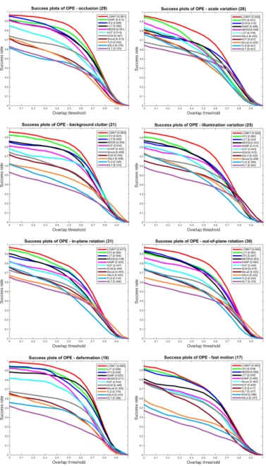
Attribute-based Evaluation: For the detailed performance analysis of each

OOTB [22] such as occlusion, scale variation, illumination variation, etc. As shown in Fig. 4, our proposed tracker outperforms the state-of-the-art trackers in almost all challenge attributes. In particular, our proposed tracker (LCMHT) 495

performs significantly better than all trackers on the occlusion attribute since it includes a re-detection module which can re-acquire the target in case the tracker fails even in cluttered environments by removing clutter using GM-PHD filter. Similarly, our tracker also outperforms other trackers on the scale variation at-tribute since our tracker elegantly estimates the scale of the tracker at the newly 500

estimated target positions. The LCT algorithm includes both re-detection and scale estimation modules, however, our proposed tracker still outperforms the LCT algorithm by a large margin as shown in Fig. 4 since our tracker uses bet-ter visual features for translation estimation and re-detection. Furthermore, our proposed algorithm applies scale estimation after translation and re-detection 505

steps (if activated) rather than only after the translation estimation step as in the LCT algorithm, though both methods use similar visual features (HOG) to learn the scale correlation filter.

Qualitative Evaluation: We compare our proposed tracking algorithm (LCMHT)

with four other state-of-the-art trackers namely CF2 [36], MEEM [21], LCT [39] 510

and KCF [28] on some challenging sequences of OOTB qualitatively as shown in Fig. 5. CF2 uses hierarchical CNN features but is not as effective as our tracker which combines hierarchical CNN features with HOG and color-naming traditional features as can be observed on the sequenceFleetface (first column on Fig. 5). LCT and KCF also use correlation filters using traditional features 515

but still they are not as accurate as our tracker. MEEM uses many classifiers together to re-initialize the tracker in case of tracking failures but it can not re-detect the target on this sequence. Similarly, it can not re-detect the target on sequencesSinger1 (second column),Freeman4 (third column) andWalking2 (forth column) as well. LCT includes re-detection and scale estimation com-520

ponents, however, it can not handle large scale changes as in sequenceSinger1 (second column), and it can not re-initialize the tracker as in sequenceWalking2 (forth column). More importantly, the sequenceFreeman4 undergoes not only

Figure 4: Success plots on OOTB using one-pass evaluation (OPE) for 8 challenge attributes: occlusion, scale variation, background clutter, illumination variation, in-plane rotation, out-of-in-plane rotation, deformation, and fast motion. The legend con-tains the AUC score of each tracker; the larger, the better.

heavy occlusion in a cluttered environment but also scale variation, in-plane and out-of-plane rotations. The LCT algorithm which is equipped with both 525

re-detection and scale estimation modules is not effective on this sequence like the other algorithms. However, only our proposed tracker tracks the target till the end of the sequence not only handling the scale change but also re-detecting the target when it fails. This sequence is a typical example which is related to our next evaluation on PETS 2009 data sets on which our proposed algorithm 530

outperforms the other trackers by a large margin.

6.2. Evaluation on PETS 2009 Data Sets

We label the upper part (head + neck) of representative targets in both medium and dense PETS 2009 data sets to analyze our proposed tracking algorithm. In this experiment, our goal is to analyze our proposed tracking algorithm and 535

other available state-of-the-art tracking algorithms to see whether they can suc-cessfully be applied for tracking a target of interest in occluded and cluttered environments. Accordingly, we compare our proposed tracking algorithm with 6 state-of-the-art trackers including CF2 [36], LCT [39], MEEM [21], DSST [29], KCF [28] and SAMF [47], as well as 4 more top trackers included in the Bench-540

mark [22], particularly SCM [26], ASLA [14], CSK [27] and IVT [15] both quan-titatively and qualitatively.

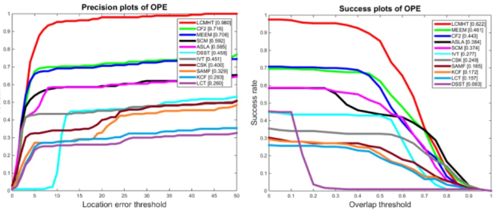
Quantitative Evaluation: The evaluation results of precision plots (left) and

success plots (right) based on center location error and bounding box overlap ratio, respectively, are shown in Fig. 6. Our proposed tracking algorithm, de-545

noted by LCMHT, outperforms the state-of-the-art trackers by a large margin on PETS 2009 data sets in both precision and success rate measures. The rank-ings are given in distance precision of threshold scores at 20 pixels and overlap success of AUC score for each tracker as given in the legends.

The second and third ranked trackers are CF2 [36] and MEEM [21] for precision 550

plots, respectively, and viceversa for success plots on PETS 2009 data sets. However, on OOTB, CF2 outperforms MEEM significantly being second to our proposed tracking algorithm. The most important thing to give attention is on

Figure 5:Qualitative results of our proposed LCMHT algorithm, CF2 [36], MEEM [21], LCT [39] and KCF [28] on some challenging sequences of OOTB (Fleetface, Singer1, Freeman4, and Walking2 from left column to right column, respectively).

the performance of LCT [39]. This algorithm is ranked third on the OOTB as shown in Fig. 3, however, it performs least well on the precision plots and second 555

from last on success plots on PETS 2009 data sets. Surprisingly, this algorithm was developed by learning three different discriminative correlation filters and even included a re-detection module for long-term tracking problems. Though it performs reasonably on the OOTB, its performance on occluded and cluttered

Figure 6:Distance precision (left) and overlap success (right) plots on PETS data sets using one-pass evaluation (OPE). The legend for distance precision contains threshold scores at 20 pixels while the legend for overlap success contains the AUC score of each tracker.

environments such as PETS 2009 data sets is poor due to using less robust 560

visual features in such environments. Even CF2 which uses CNN features has low performance compared to our proposed algorithm on the PETS 2009 data sets. Since our proposed tracking algorithm integrates a hybrid of multi-layer CNN and traditional features for learning the translation correlation filter and GM-PHD filter for temporally filtering generated high score detection proposals 565

during a re-detection phase for removing clutter, it outperforms all the available trackers significantly. This closes the model-free tracking research gap between sparse and crowded environments.

Qualitative Evaluation: Fig. 7 presents the performance of our proposed

tracker qualitatively compared to the state-of-the-art trackers. In this case, we 570

show the comparison of four representative trackers to our proposed algorithm: CF2 [36], MEEM [21], LCT [39], and KCF [28] as shown in Fig 7. On the medium density PETS 2009 data set (left column), LCT and KCF lose the target even on the first 16 frames. Though, the CF2 and MEEM trackers track the target well, they could not re-detect the target after the occlusion i.e. only 575

by re-initializing the tracker after the occlusion. We show the cropped and enlarged re-detection just after occlusion in Fig. 8. On the dense PETS data set (right column), all trackers track the target on the first 20 frames but LCT and KCF lose the target before 73 frames. Similar to the medium density PETS 580

data set, the CF2 and MEEM trackers track the target before they lose it due to occlusion. Only our proposed tracking algorithm, LCMHT, re-detects the target and tracks it till the end of the sequence in such dense environments due to two reasons. First, it incorporates both lower and higher CNN layers in combination with traditional features (HOG and color-naming) in a multi-layer to learn the 585

translation correlation filter that is robust to appearance variations of targets. Second, it includes a re-detection module which generates high score detection proposals during a re-detection phase and then filter them using GM-PHD filter to remove clutter due to background and other uninterested targets so that it can re-detect the target in such cluttered and dense environment. These make 590

our proposed tracking algorithm outperform the other state-of-the-art trackers.

7. Conclusions

We have developed a novel long-term visual tracking algorithm by learning dis-criminative correlation filters and an incremental SVM classifier that can be applied for tracking of a target of interest in sparse as well as in crowded envi-595

ronments. We learn two different discriminative correlation filters: translation and scale correlation filters. For the translation correlation filter, we combine a hybrid of multi-layer CNN features trained on a large amount of object recog-nition data set (ImageNet) and traditional (HOG and color-naming) features in proper proportion. For the CNN part, we combine the advantages of both lower 600

and higher convolutional layers to capture spatial details for precise localiza-tion and semantic informalocaliza-tion for handling appearance varialocaliza-tions, respectively. We also include a re-detection module using HOG, LUV color and normalized gradient magnitude features for re-initializing the tracker in case of tracking failures due to long-term occlusions by training an incremental SVM from the 605

Figure 7:Qualitative results of our proposed algorithm LCMHT, CF2 [36], MEEM [21], LCT [39] and KCF [28] on PETS 2009 medium density (left column) and dense (right column) data sets.

Figure 8:Qualitative results of our proposed LCMHT algorithm, CF2 [36], MEEM [21], LCT [39] and KCF [28] on PETS 2009 medium density (left, frame 78) and dense (right, frame 85) data sets, just after occlusion by cropping and enlarging.

most confident frames. The re-detection module generates high score detection proposals which are temporally filtered using a GM-PHD filter for removing clutter. The Gaussian component with maximum weight is selected as a state estimate which re-fines the object location when a re-detection module is ac-tivated. For the scale correlation filter, we use HOG features to construct a 610

target pyramid around the estimated or re-detected position for estimating the scale of the target. Extensive experiments on both OOTB and PETS 2009 data sets show that our proposed algorithm significantly outperforms state-of-the-art trackers by 3.48% in distance precision and 7.77% in overlap success on sparse (OOTB) data sets, and by 36.87% in distance precision and 34.92% in overlap 615

success on dense (PETS 2009) data sets. We conclude that learning correlation filters using an appropriate combination of CNN and traditional features as well as including a re-detection module using incremental SVM and GM-PHD filter can give better results than many existing approaches.

Acknowledgment

620

We would like to acknowledge the support of the Engineering and Physical Sciences Research Council (EPSRC), grant references EP/K009931 and a James Watt Scholarship.

References

[1] A. W. M. Smeulders, D. M. Chu, R. Cucchiara, S. Calderara, A. Dehghan, 625

M. Shah, Visual tracking: An experimental survey, IEEE Transactions on Pattern Analysis and Machine Intelligence 36 (7) (2014) 1442–1468.

[2] H. Yang, L. Shao, F. Zheng, L. Wang, Z. Song, Recent advances and trends in visual tracking: A review, Neurocomputing 74 (18) (2011) 3823 – 3831.

[3] R. Girshick, J. Donahue, T. Darrell, J. Malik, Rich feature hierarchies for 630

accurate object detection and semantic segmentation, in: Computer Vision and Pattern Recognition, 2014.

[4] K. Simonyan, A. Zisserman, Very deep convolutional networks for large-scale image recognition, ICLR.

[5] N. Wang, D.-Y. Yeung, Learning a deep compact image representation for 635

visual tracking, in: C. J. C. Burges, L. Bottou, M. Welling, Z. Ghahramani, K. Q. Weinberger (Eds.), Advances in Neural Information Processing Sys-tems 26, 2013, pp. 809–817.

[6] S. Hong, T. You, S. Kwak, B. Han, Online tracking by learning discrimina-tive saliency map with convolutional neural network, in: Proceedings of the 640

32nd International Conference on Machine Learning, 2015, Lille, France, 6-11 July 2015, 2015.

[7] Z. Chen, Z. Hong, D. Tao, An experimental survey on correlation filter-based tracking, CoRR abs/1509.05520.

[8] B.-N. Vo, W.-K. Ma, The Gaussian mixture probability hypothesis density 645

filter, Signal Processing, IEEE Transactions on 54 (11) (2006) 4091–4104.

[9] N. L. Baisa, A. Wallace, Multiple Target, Multiple Type Filtering in RFS Framework, ArXiv e-printsarXiv:1705.04757.

[10] N. L. Baisa, A. Wallace, Multiple target, multiple type visual tracking using a Tri-GM-PHD Filter, in: Proceedings of the 12th International Conference 650

on Computer Vision Theory and Applications (VISAPP), VISIGRAPP, 2017.

[11] N. L. Baisa, D. Bhowmik, A. Wallace, Long-term correlation tracking using multi-layer hybrid features in dense environments, in: Proceedings of the 12th International Conference on Computer Vision Theory and Applica-655

tions (VISAPP), VISIGRAPP, 2017.

[12] B. Han, D. Comaniciu, Y. Zhu, L. S. Davis, Sequential kernel density ap-proximation and its application to real-time visual tracking, IEEE Trans-actions on Pattern Analysis and Machine Intelligence 30 (7) (2008) 1186– 1197.

660

[13] T. Zhang, B. Ghanem, S. Liu, N. Ahuja, Robust visual tracking via multi-task sparse learning, in: Computer Vision and Pattern Recognition (CVPR), 2012 IEEE Conference on, 2012, pp. 2042–2049.

[14] X. Jia, H. Lu, M. H. Yang, Visual tracking via adaptive structural local sparse appearance model, in: Computer Vision and Pattern Recognition 665

(CVPR), 2012 IEEE Conference on, 2012, pp. 1822–1829.

[15] D. A. Ross, J. Lim, R.-S. Lin, M.-H. Yang, Incremental learning for robust visual tracking, International Journal of Computer Vision 77 (1) (2008) 125–141.

[16] H. Grabner, C. Leistner, H. Bischof, Semi-supervised on-line boosting for 670

robust tracking, in: Proceedings of the 10th European Conference on Com-puter Vision: Part I, ECCV ’08, 2008, pp. 234–247.

[17] B. Babenko, M. H. Yang, S. Belongie, Robust object tracking with online multiple instance learning, IEEE Transactions on Pattern Analysis and Machine Intelligence 33 (8) (2011) 1619–1632.

675

[18] Z. Kalal, K. Mikolajczyk, J. Matas, Tracking-learning-detection, IEEE Transactions on Pattern Analysis and Machine Intelligence 34 (7) (2012) 1409–1422.

[19] J. Gao, H. Ling, W. Hu, J. Xing, Transfer learning based visual tracking with gaussian processes regression, in: Computer Vision - ECCV, 2014, pp. 680

188–203.

[20] S. Hare, A. Saffari, P. H. S. Torr, Struck: Structured output tracking with kernels, in: 2011 International Conference on Computer Vision, 2011, pp. 263–270.

[21] J. Zhang, S. Ma, S. Sclaroff, MEEM: robust tracking via multiple experts 685

using entropy minimization, in: Proc. of the European Conference on Com-puter Vision (ECCV), 2014.

[22] Y. Wu, J. Lim, M. H. Yang, Online object tracking: A benchmark, in: Computer Vision and Pattern Recognition (CVPR), 2013 IEEE Conference on, 2013, pp. 2411–2418.

690

[23] Y. Wu, J. Lim, M. H. Yang, Object tracking benchmark, IEEE Transactions on Pattern Analysis and Machine Intelligence 37 (9) (2015) 1834–1848.

[24] T. Minka, Discriminative models, not discriminative training, Tech. rep. (October 2005).

[25] T. B. Dinh, Q. Yu, G. Medioni, Co-trained generative and discrimina-695

tive trackers with cascade particle filter, Comput. Vis. Image Underst. 119 (2014) 41–56.

[26] W. Zhong, H. Lu, M. H. Yang, Robust object tracking via sparsity-based collaborative model, in: Computer Vision and Pattern Recognition (CVPR), 2012 IEEE Conference on, 2012, pp. 1838–1845.

700

[27] J. a. F. Henriques, R. Caseiro, P. Martins, J. Batista, Exploiting the cir-culant structure of tracking-by-detection with kernels, in: Proceedings of the 12th European Conference on Computer Vision - Volume Part IV, ECCV’12, 2012, pp. 702–715.

[28] J. F. Henriques, R. Caseiro, P. Martins, J. Batista, High-speed tracking 705

with kernelized correlation filters, Pattern Analysis and Machine Intelli-gence, IEEE Transactions on.

[29] M. Danelljan, G. Hager, F. Shahbaz Khan, M. Felsberg, Accurate scale es-timation for robust visual tracking, in: Proceedings of the British Machine Vision Conference, BMVA Press, 2014.

710

[30] Q. Wang, A. Alfalou, C. Brosseau, New perspectives in face correlation research: a tutorial, Adv. Opt. Photon. 9 (1) (2017) 1–78.

[31] A. Alfalou, C. Brosseau, Chapter two - recent advances in optical image processing, Vol. 60 of Progress in Optics, Elsevier, 2015, pp. 119 – 262.

[32] F. Bouzidi, M. Elbouz, A. Alfalou, C. Brosseau, A. Fakhfakh, Optimization 715

of the performances of correlation filters by pre-processing the input plane, Optics Communications 358 (Complete) (2016) 132–139.

[33] D. Benarab, T. Napolon, A. Alfalou, A. Verney, P. Hellard, Optimized swimmer tracking system based on a novel multi-related-targets approach, Optics and Lasers in Engineering 89 (2017) 195 – 202, 3DIM-DS 2015: 720

Optical Image Processing in the context of 3D Imaging, Metrology, and Data Security.

[34] T. Napolon, A. Alfalou, Pose invariant face recognition: 3D model from sin-gle photo, Optics and Lasers in Engineering 89 (2017) 150 – 161, 3DIM-DS 2015: Optical Image Processing in the context of 3D Imaging, Metrology, 725

and Data Security.

[35] Y. Ouerhani, A. Alfalou, M. Desthieux, C. Brosseau, Advanced driver as-sistance system: Road sign identification using VIAPIX system and a cor-relation technique, Optics and Lasers in Engineering 89 (2017) 184 – 194, 3DIM-DS 2015: Optical Image Processing in the context of 3D Imaging, 730

[36] C. Ma, J. B. Huang, X. Yang, M. H. Yang, Hierarchical convolutional features for visual tracking, in: 2015 IEEE International Conference on Computer Vision (ICCV), 2015, pp. 3074–3082.

[37] K. Zhang, L. Zhang, Q. Liu, D. Zhang, M. Yang, Fast visual tracking via 735

dense spatio-temporal context learning, in: Computer Vision - ECCV 2014 - 13th European Conference, Zurich, Switzerland, September 6-12, 2014, Proceedings, Part V, 2014, pp. 127–141.

[38] L. Wang, W. Ouyang, X. Wang, H. Lu, Visual tracking with fully convo-lutional networks, in: 2015 IEEE International Conference on Computer 740

Vision (ICCV), 2015, pp. 3119–3127.

[39] C. Ma, X. Yang, C. Zhang, M. H. Yang, Long-term correlation tracking, in: 2015 IEEE Conference on Computer Vision and Pattern Recognition (CVPR), 2015, pp. 5388–5396.

[40] H. Nam, B. Han, Learning multi-domain convolutional neural networks for 745

visual tracking, CoRR abs/1510.07945.

[41] M. Rodriguez, J. Sivic, I. Laptev, J.-Y. Audibert, Density-aware person detection and tracking in crowds.

[42] L. Kratz, K. Nishino, Tracking pedestrians using local spatio-temporal mo-tion patterns in extremely crowded scenes, IEEE Transacmo-tions on Pattern 750

Analysis and Machine Intelligence 34 (5) (2012) 987–1002.

[43] H. Idrees, N. Warner, M. Shah, Tracking in dense crowds using prominence and neighborhood motion concurrence, Image and Vision Computing 32 (1) 14.

[44] P. F. Felzenszwalb, R. B. Girshick, D. McAllester, D. Ramanan, Object de-755

tection with discriminatively trained part based models, IEEE Transactions on Pattern Analysis and Machine Intelligence 32 (9) (2010) 1627–1645.

[45] J. van de Weijer, C. Schmid, J. Verbeek, D. Larlus, Learning color names for real-world applications, Trans. Img. Proc. 18 (7) (2009) 1512–1523.

[46] F. S. Khan, R. M. Anwer, J. van de Weijer, A. D. Bagdanov, M. Vanrell, 760

A. M. L´opez, Color attributes for object detection, in: IEEE Conference on Computer Vision and Pattern Recognition, Providence, RI, USA, June 16-21, 2012, pp. 3306–3313.

[47] Y. Li, J. Zhu, A Scale Adaptive Kernel Correlation Filter Tracker with Feature Integration, Springer International Publishing, Cham, 2015, Ch. 765

Computer Vision - ECCV 2014 Workshops: Zurich, Switzerland, Septem-ber 6-7 and 12, 2014, Proceedings, Part II, pp. 254–265.

[48] R. Rifkin, G. Yeo, T. Poggio, Regularized least-squares classification, Nato Science Series Sub Series III Computer and Systems Sciences 190 (2003) 131–154.

770

[49] K. P. Murphy, Machine Learning: A Probabilistic Perspective, The MIT Press, 2012.

[50] C. P. Diehl, G. Cauwenberghs, SVM incremental learning, adaptation and optimization, in: Neural Networks, 2003. Proceedings of the International Joint Conference on, Vol. 4, 2003, pp. 2685–2690 vol.4.

775

[51] B. Ristic, D. E. Clark, B.-N. Vo, B.-T. Vo, Adaptive target birth intensity for PHD and CPHD filters, IEEE Transactions on Aerospace and Electronic Systems 48 (2) (2012) 1656–1668.

[52] J. Deng, W. Dong, R. Socher, L. J. Li, K. Li, L. Fei-Fei, ImageNet: A large-scale hierarchical image database, in: Computer Vision and Pattern 780

Recognition, 2009. CVPR 2009. IEEE Conference on, 2009, pp. 248–255.

[53] A. Vedaldi, K. Lenc, MatConvNet – convolutional neural networks for mat-lab, in: Proceedings of the 25th annual ACM international conference on Multimedia, 2015.