Ecological Modelling

(1)

Contents lists available atScienceDirect

Ecological Modelling

j o u r n a l h o m e p a g e :w w w . e l s e v i e r . c o m / l o c a t e / e c o l m o d e l

Using social network analysis tools in ecology: Markov process transition models

applied to the seasonal trophic network dynamics of the Chesapeake Bay

Jeffrey C. Johnson

a

_{, Joseph J. Luczkovich}

b,∗

_{, Stephen P. Borgatti}

c

_{, Tom A.B. Snijders}

d,e a_{Sociology Department and Institute for Coastal Science and Policy, East Carolina University, Greenville, NC 27858, USA}

b_{Biology Department and Institute for Coastal Science and Policy, East Carolina University, 383 Flanagan, Greenville, NC 27858, USA} c_{Department of Management, University of Kentucky, Lexington, KY, USA}

d_{Department of Statistics, University of Oxford, United Kingdom}

e_{ICS, Department of Sociology, University of Groningen, Grote Rozenstraat 31, 9712 TG Groningen, The Netherlands}

a r t i c l e i n f o

Article history:

Available online 24 August 2009

Keywords:

Estuary Ascendency

Continuous-time Markov model Dynamics

Statistical network analysis Network visualization

a b s t r a c t

Ecosystem components interact in complex ways and change over time due to a variety of both inter-nal and exterinter-nal influences (climate change, season cycles, human impacts). Such processes need to be modeled dynamically using appropriate statistical methods for assessing change in network structure. Here we use visualizations and statistical models of network dynamics to understand seasonal changes in the trophic network model described by Baird and Ulanowicz [Baird, D., Ulanowicz, R.E., 1989. Seasonal dynamics of the Chesapeake Bay ecosystem. Ecol. Monogr. 501 (59), 329–364] for the Chesapeake Bay (USA). Visualizations of carbon flow networks were created for each season by using a network graphic analysis tool (NETDRAW). The structural relations of the pelagic and benthic compartments (nodes) in each seasonal network were displayed in a two-dimensional space using spring-embedder analyses with nodes color-coded for habitat associations (benthic or pelagic). The most complex network was summer, when pelagic species such as sea nettles, larval fishes, and carnivorous fishes immigrate into Chesapeake Bay and consume prey largely from the plankton and to some extent the benthos. Winter was the sim-plest of the seasonal networks, and exhibited the highest ascendency, with fewest nodes present and with most of the flows shifting to the benthic bacteria and sediment POC compartments. This shift in system complexity corresponds with a shift from a pelagic- to benthic-dominated system over the seasonal cycle, suggesting that winter is a mostly closed system, relying on internal cycling rather than external input. Network visualization tools are useful in assessing temporal and spatial changes in food web networks, which can be explored for patterns that can be tested using statistical approaches. A simulation-based continuous-time Markov Chain model called SIENA was used to determine the dynamic structural changes in the trophic network across phases of the annual cycle in a statistical as opposed to a visual assessment. There was a significant decrease in outdegree (prey nodes with reduced link density) and an increase in the number of transitive triples (a triad in whichichoosesjandh, andjalso choosesh, mostly connected via the non-living detritus nodes in positioni), suggesting the Chesapeake Bay is a simpler, but structurally more efficient, ecosystem in the winter than in the summer. As in the visual analysis, this shift in system complexity corresponds with a shift from a pelagic to a more benthic-dominated system from summer to winter. Both the SIENA model and the visualization in NETDRAW support the conclusions of Baird and Ulanowicz [Baird, D., Ulanowicz, R.E., 1989. Seasonal dynamics of the Chesapeake Bay ecosystem. Ecol. Monogr. 501 (59), 329–364] that there was an increase in the Chesapeake Bay ecosystem’s ascendancy in the winter. We explain such reduced complexity in winter as a system response to lowered temperature and decreased solar energy input, which causes a decline in the production of new carbon, forcing nodes to go extinct; this causes a change in the structure of the system, making it simpler and more efficient than in summer. It appears that the seasonal dynamics of the trophic structure of Chesapeake Bay can be modeled effectively using the SIENA statistical model for network change.

∗ _{Corresponding author. Tel.: +1 252 328 9402; fax: +1 252 328 4178.}

E-mail addresses:[email protected](J.J. Luczkovich),[email protected] (S.P. Borgatti).

1. Introduction

Ecosystem components interact in complex ways and change over time due to a variety of both endogenous and exogenous inﬂuences (e.g., season cycles, human impacts). Past work on food

(2)

webs has been mostly descriptive and deterministic (Polis and Winemiller, 1996). Models of empirical food webs were largely static, based on data collected at a single point in time, or more typ-ically, based on averaged data taken on a seasonal or annual basis. Such static models are not appropriate for understanding dynamic processes over time.

The use of dynamic modeling approaches for analyzing food webs has been described in two recent books (de Ruiter et al., 2005; Belgrano et al., 2005; Pascual and Dunne, 2006). These dynamic models are based on simulated populations of species and their potential trophic interactions, in which populations grow or shrink over time depending upon the structure of the network (represented as a matrix indicating the species each other species consumes). Various parameters determine popula-tion growth, predapopula-tion rates, interacpopula-tion strengths, and predator switching behaviors. The models attempt to recreate and match empirically derived structural characteristics of ecological net-works [e.g., the cascade model (Cohen and Newman, 1985), the generalized niche model (Williams and Martinez, 2000), the phy-logenetic constraint model (Cattin et al., 2004) and the minimum potential niche model (Allesina et al., 2008)]. These models or their variants have been used to examine the system stability in the face of changes in the removal and addition of species (for a review of the complexity–stability debate, seeDunne et al., 2005; McCann et al., 2005). Many of these dynamic simulations are unrealistic. For example, some fail to include detritus. And in many cases, the models cannot be used to assess whether changes in the structure of observed trophic networks over time are statistically signiﬁcant. An alternative approach is based on modeling changes in observed network properties over time using empirically measured trophic networks. In a trophic network, or food web, the nodes are species or groups of species (compartments), and a tie from one node to another denotes a carbon ﬂow, or a predator–prey relation. Empirical data on certain food webs are collected over time, pro-viding temporal data sets for examination of food web dynamics, and these are typically analyzed using ecological network analy-sis software (e.g., Ecopath, Netwrk). The resulting measures are then presented as a series of whole ecosystem measures like ascen-dency (Baird and Ulanowicz, 1989; Baird et al., 1998; Baird and Heymans, 1996; Ulanowicz and Robert, 2001; Scharler and Baird, 2005; Heymans et al., 2007). These models are based on “snapshots” of actually observed (as opposed to potential) species interactions in ecosystems and describe how the properties of the networks change over time, and thus offer a basis for realistic description of ecosystem network dynamics. Because these models are based on real ecosystem measurements, they have great potential to yield insight for whole system behavior and ecosystem management.

However, time series analyses of high-level network measures do not model the patterns of species–species interactions at a fun-damental level. As a result, they cannot answer basic questions that we would like to pose. For example, when is a food web observed at one time period signiﬁcantly different than one observed at a later time? What attributes (habitat occupied, reproductive or juvenile life stage, defensive chemicals, morphology, behavior, body size, etc.) of each species are associated with these ecosystem changes? When an external perturbation has occurred (like the construction of a dam, harvest, introduction or removal of species, or a seasonal or climate change), does the food web network shift signiﬁcantly to a new topology or structure afterward?

Analogous problems have been approached in the social sci-ences in the analysis of social networks. Social scientists have examined dynamically changing social networks as people enter and leave groups and form and dissolve relationships. One impor-tant approach (Snijders, 2001; Huisman and Snijders, 2003), based on a continuous-time Markov chain model, conceptualizes pair-wise interactions among nodes in a network as a function of a set

of parameters corresponding to tendencies to form certain micro-structural conﬁgurations or motifs. Given longitudinal data, the parameters and their standard errors can be estimated, enabling statistical tests of differences in parameters across networks or over time. We suggest that this social science methodology can be effective in ecological settings as well, provided care is taken in the selection of parameters and interpretation of results

1.1. Previous use of Markov approaches in ecology

Markov chains are stochastic models of the possible paths that the states of any system can follow. Given a current state of the system, transitional probabilities are estimated that govern the like-lihood of transitioning to another state. A deﬁning characteristic of Markov models is that the probability of entering a given state at timetis solely a function of the current state. A simple example is a random walk Markov model in which the states of a system are represented as nodes in a graph, and the next state is chosen at ran-dom from the set of neighbors of the current node. No information is needed about the history of the walk.

Markov approaches have been used previously in population and community ecology to model species’ population growth and interactions. One instance, called the Leslie matrix, is an age-based population model in which the number of individuals in multiple age classes is used to model the transition probabilities of individu-als surviving to the next age class in each time step (e.g.,Mollet and Cailliet, 2002). Markov models have been used to study competitive networks of species (Buss and Jackson, 1979), diversity–stability relationships in ecosystems (Li and Charnov, 2001), and to model transition probabilities of species surviving in rocky intertidal com-munities (Wootton, 2001). There has not been an attempt to use the continuous-time Markov chain approach to study food web net-work dynamics (de Ruiter et al., 2005). Most of these approaches are discrete-time Markov models in which they assume equilibrium or steady-state conditions (e.g., the transition probabilities do not change over time). In a continuous-time Markov model, the states occur in a time sequence and the transition probabilities can change continuously over time.

1.2. SIENA model

Snijders (2001)andHuisman and Snijders (2003)have recently introduced a family of continuous-time Markov chain models (CTMCM) for investigating the evolution of social networks known as the SIENA model. The model is implemented in a well-known computer program of the same name, SIENA (Simulation Investi-gation for Empirical Network Analysis)Snijders et al. (2007). The models speciﬁcally address both change in network structure (who has ties to whom) and changes in node attributes (such as behav-ior or body size). The basic principle underlying the SIENA model is that changes in directed network ties are made as a function of a node-level utility function – similar to those found in optimal foraging theory – whose parameters the model estimates. Thus, changes in the structure of the food web are modeled in terms of changes in individual nodes’ behaviors as they maximize their utility functions. The idea is that because predators consume prey preferentially and exhibit prey switching behavior, this process cre-ates a new network structure of trophic interactions at each time period. The observed changes in the network are then used to esti-mate the parameters of the process theorized to underlie these changes.

At a larger level, the model conceptualizes change in terms of transitions between states in a state space that consists of all possi-ble combinations of network conﬁgurations (and, optionally, node attributes). Because of the complexity and magnitude of possible transitions under these conditions, the model makes three

(3)

sim-plifying assumptions. First, as in any Markov process, transition probabilities depend solely on the current state, rather than on a past trajectory over time. Second, there is a micro-step restric-tion that network nodes can only make changes in one network tie or behavior at a time. This means that all changes in the network are sequential, and are not allowed to be simultaneous. This is a restriction which makes modeling simpler because it breaks down changes in the smallest possible steps. Finally, nodes make choices independent of other node’s choices, conditional on the current state of the system as a whole.

Applied to trophic networks, the SIENA model takes as input a set of binary matrices of species interactions at each time period. The probability of transitioning from one predator- and prey-relation state to another is modeled for all species across all time periods. The structure of the food web evolves as the constituent species make changes in response to their local situations, such as changing prey abundance.

Implicit in the model is the notion that species choose their prey non-randomly (see, for example,Dell et al., 2005), reflect-ing tendencies toward this or that micro-configuration. Models are specified in SIENA by selecting these micro-structures or motifs – known as effects – that reflect structural characteristics of theoreti-cal interest in modeling network dynamics. For example, in human networks, there is a strong tendency for positive ties such as friend-ship to be reciprocated: ifinamesjas a friend, there is an increased likelihood thatjnamesias a friend. In food webs, we expect the opposite effect: if speciesipreys on speciesj, it is unusual (but not impossible) forjto prey oni. To apply SIENA in a given research project, it is important to select theoretically meaningful param-eters that are relevant to the setting (e.g., food webs) and to the theoretical questions. For example, one effect available in SIENA is “outdegree” which reflects the tendency of a node to have ties to many other nodes. Thus, outdegree represents prey diversity and is strongly related to network connectance. Another relevant objec-tive function is the number of transiobjec-tive triples (in which species

ieatsj, speciesjeats speciesk, and species ieats speciesk). A tendency toward transitive triples indicates omnivory—feeding at multiple trophic levels.

The output of the SIENA model consists of a set of estimates of the parameters, along with their standard errors. This allows us to statistically test effects that are hypothesized to be among the driving forces of dynamics of networks over time. The idea is that because predators consume prey preferentially, exhibit prey switching behavior, and choose different prey over time, this pro-cess creates a new network of trophic interactions at each time period. As a null model, the CTCMC approach simulates the evo-lution of the structure of networks by creating many such random trophic networks, allowing predators to change a single new prey link randomly at each time period. These simulations of random network evolution then serve as a null model to test the observed distribution of trophic links in an actual ecosystem. By doing this, we can compare ecological measures of the resulting networks (e.g., organizational metrics like ascendency, connectance, link den-sity, cycling, indirect relations, preferential attachment of predators during network evolution, similarity of node attributes of interact-ing species, etc.) against the null distribution of random networks, allowing for a statistical tests of network structural properties over time.

1.3. Example: Chesapeake Bay ecological network data

We illustrate the SIENA methodology by applying it to the Chesa-peake Bay carbon ﬂow network ofBaird and Ulanowicz (1989). A series of seasonal food webs of the Chesapeake Bay, originally described byBaird and Ulanowicz (1989), were modeled using the carbon ﬂow in a 36-compartment food web of the Chesapeake Bay

Table 1

A list of the living and non-living compartments in the Chesapeake Bay network model used byBaird and Ulanowicz (1989)and their numerical identiﬁers. Living compartments

1 Phytoplankton

2 Bacteria in suspended particulate organic carbon (suspPOC) 3 Bacteria in sediment particulate organic carbon (sedPOC) 4 Benthic diatoms

5 Free bacteria

6 Heterotrophic microﬂagellates 7 Ciliates

8 Zooplankton

9 CtenophoresMnemiopsis leidyi 10 Sea NettleChrysaora quinquercirrha 11 Other suspension feeders 12 ClamMya arenaria 13 OystersCrassostrea virginica 14 Other polychaetes 15 PolychaeteNereissp. 16 ClamMacomaspp. 17 Meiofauna

18 Crustacean deposit feeder 19 Blue crabCallinectes sapidus 20 Fish larvae

21 Alewife and Blue HerringAlosa pseudoharengusandA. aestivalis 22 Bay AnchovyAnchoa mitchilli

23 MenhadenBrevoortia tyrannus 24 American ShadAlosa sapidissima 25 Atlantic CroakerMicropogonias undulates 26 HogchokerTrinectes maculates 27 SpotLeiostomus xanthurus 28 White PerchMorone americana 29 Hardhead CatfishArias felis 30 BluefishPomatomus saltatrix 31 WeakfishCynoscion regalis

32 Summer FlounderParalichthys dentatus 33 Striped BassMorone saxatilis Non-living compartments

34 Dissolved organic carbon (DOC)

35 Suspended particulate organic matter (SusPOM) 36 Sediment particulate organic matter (SedPOM)

(Table 1). The model was originally constructed from published data to reflect the measured seasonal changes in carbon flow among the compartments. Due to migrations and seasonal fluctuations in abundance, the model had 33 compartments in spring, 36 in summer, 32 in fall, and 28 in winter. Species diversity increased from the spring to summer, reaching the maximum then as sev-eral new species developed or migrated into the system. Diversity was lowest in the winter. In the summer, the system was a pelagic-fish- and plankton-dominated system, with gelatinous zooplankton becoming the dominant group. In the winter, the system was dom-inated by flows within the detritus and benthos compartments.

Baird and Ulanowicz (1989)concluded that the Chesapeake’s sys-tem throughput and respiration was greatest in summer and lowest in winter, but that system organization as measured by ascendency (average mutual information in the system normalized by through-put) was greatest in winter, least in summer. They wrote: “These quantitative results recapitulate the intuitive notion that carbon ﬂow dynamics in the Chesapeake Bay during the summer are both dissipa-tive and less organized than those during the less acdissipa-tive, cooler seasons” (Baird and Ulanowicz, 1989, p. 355).

To illustrate the method, we have simpliﬁed the Baird and Ulanowicz dataset by dichotomizing and transposing the carbon ﬂow matrix to create a binary diet matrix Xin which Xij= 1 if

compartment i feeds on compartment j, and Xij= 0 otherwise.

Dichotomizing the data simpliﬁes the interpretation of the model, but of course results in reduced realism. Even so, the analysis should reveal the major organizational and structural changes in the sea-sonal shifts in the ecosystem, and allow us to test the structural implications of the theoretical assertions advanced by Baird and

(4)

Ulanowicz, such as increasing ascendency. It is also important to note that the SIENA method can, in principle, also be applied to networks with weighted links (e.g., representing carbon ﬂows), although there are some conceptual complexities with this that lie outside the scope of this paper.

1.4. Objectives

We will conduct a dynamic statistical analysis of the process of seasonal change in network structure of the Chesapeake Bay as it changes seasonally, with particular reference to the changes in sys-tem organization that occurred across seasons (e.g., the increased ascendency in winter) that were observed byBaird and Ulanowicz (1989). In doing this statistical analysis of seasonal change in system organization, we will also address the following questions: (1) does the ecosystem trophic network change over time? (2) What are the network structural characteristics of ecological interest, and how do they change across seasons? (3) How does system complexity change over time? (4) What happens when species are added or leave the system (seasonal migration of some species of transient ﬁshes and invertebrates)?

2. Methods

We use a combination of graphical (visualization of the network with NETDRAW, with species or compartments as nodes and arrows showing carbon ﬂows) and quantitative methods (SIENA model of binary relations) to explore the Chesapeake Bay seasonal data.

2.1. Visualizations

Network drawing software such as NETDRAW (Borgatti, 2002) enables us to visualize changes in networks in a holistic, qualita-tive manner. We advocate visualization as an aid to interpreting and checking the SIENA model output. Here we used NETDRAW’s spring-embedding algorithmEades (1984). The algorithm concep-tualizes the network as objects interconnected by springs which require energy to pull apart but also push back if nodes get too close. The algorithm begins by arranging the nodes randomly in space, and then begins moving them in such a way as to minimize energy (Gajer and Kobourov, 2002). In general, this algorithm results in a layout in which nodes with the greatest link density are at the center of the plot and nodes that are more isolated are on the periphery.

For the sake of these visualizations and to be in keeping with the original network analysis, carbon ﬂow in mg C m−2_yr−1 _for

each season was imported from the Network program ofBaird and Ulanowicz (1989). An attribute file was created that listed for each node whether it was found in the pelagic realm or the ben-thic habitats of Chesapeake Bay. These nodes and their carbon flow links were graphed using the spring-embedder algorithm of NET-DRAW to arrange the nodes. Nodes were color-coded for habitat associations (pelagic or benthic). The line thickness was set to be proportional to carbon flow with arrows pointing from the carbon producing node (prey) to the consumer of the carbon.

2.2. SIENA analysis

We used Version 3.17s of the SIENA program, which forms part of a larger suite of software for analyzing social networks called StocNet, available on the web.1

The speciﬁcation of the model is as follows:

1_{http://stat.gamma.rug.nl/siena.html.}

(1)A continuous-time parameter. Time series overMobserved times

t1<. . .<tm<. . . tM Although modeled in continuous-time, it

is observed in discrete units tm, m= 1, . . ., M. Here seasons:

spring–summer (t1−t2), summer–fall (t2−t3), fall–winter

(t3−t4).

(2)A set of nodes(compartments)I={1,. . .,n}.

(3)Outcome space of possible networks of relations among nodes (compartments), X. The networks are time-dependent n×n

adjacency matrices.

(4)Node (compartment)-dependent attributes V and pair-dependent (dyadic) attributes W. Attributes can be constant or can vary across time.

The model examines two simultaneous dimensions, the rate of change and the direction of change. The model assumes that links in the food web change in steps where a single link may be changed. The submodel for such a step is that one predatoriis randomly chosen, and either creates a new outgoing link (i.e., chooses one additional prey), terminates one existing link (i.e., stops consum-ing one current prey), or keeps the current situation. Thus, given the choice of the predatori, there aren possibilities, composed ofn−1 changes and one non-change. The step should therefore be regarded as an opportunity for change rather than certainty of a change. The probability of each of thesen possibilities is pro-portional to exp(fi(x)) wherexis the network that would obtain

after this change (or non-change) andfi(x) is the so-called objective

function. Thus the objective function may be regarded as a utility function of the system that the predators try to maximize, with ran-dom perturbations, so that the change is not deterministic but has a probabilistic tendency to move into a direction of higher objec-tive functions. This, however, yields a rather complex model that prohibits direct calculations. Therefore, the model is implemented using a simulation approach whereby parameter estimates are pro-duced through an iterative Monte Carlo procedure based on method of moments estimation (Snijders, 2001). The objective function is represented as a weighted sum,

k

ˇksik(x) (1)

wheresik(x) are statistics driving the prey selection, andˇkare

sta-tistical weights to be estimated from the data. The parametersˇk

are non-standardized coefﬁcients. The choice of statistics for mod-eling the food web dynamics was made as follows, in accordance with basic notions in network modeling.

1.Outdegree: the outdegree of predator i, i.e., number of prey species eaten byi.

si1(x)=

j

xij (2)

2.Indegree popularity: the sum of indegrees of all the prey of preda-tori, i.e., the total number of other predators who also are preying on the prey ofi. si2(x)=

j xij

h xhj (3)

An increase in this effect indicates a stronger tendency to prey on those compartments that already have a high number of preda-tors; the weight for this effect will reﬂect level and tendency of indegree variance of the food web.

3.Transitive triplets: the number of transitive triplets with predator

(5)

such thatieatsjandhbut alsojeatsh. si3(x)=

j

h xijxjhXih (4)

This reﬂects a measure of network closure or clustering. Ecolog-ically, this will reﬂect tendencies toward omnivory.

Weights for several other statistics were estimated in an explo-rative stage, but these were not signiﬁcant and led to over-ﬁtting for this relatively small data set, as evidenced by high standard errors. The other statistics explored included a tendency to avoid reciprocity (whereieatsjbut alsojeatsi); a tendency of those compartments that prey on many other compartments (‘high out-degree’ after transposition) to continue preying on many, or even more compartments; and differential preferences between benthic and pelagic species.

2.3. Model estimation using a Monte Carlo procedure

The mathematical details of the estimation procedure can be found inSnijders (2001). The system of equations for the parame-ter estimates cannot be solved analytically or numerically. Thus, a stochastic approximation is used based on an approximation of moment estimates through a simulation of random adjacency matrices depending on provisional values of the parametersˇk. The

parameter estimates are iteratively updated in repeated simula-tions of the adjacency matrices. To allow for differentiation between the ecosystem dynamics across the seasons, the model was esti-mated for each of the three transitions spring to summer, summer to fall, and fall to winter. Parameters can be tested by Wald tests, i.e., testing the ratio of parameter estimate to standard deviation in the standard normal distribution.

In all analyses, we have restricted the outdegree (or consump-tion) relations of producers [phytoplankton (node 1) and benthic diatoms (4)] ﬁxing these as 0s (structural zeros). In this way, they are constrained to be non-feeding nodes. Such an analysis mim-ics ecological realities of producers in that they can be chosen as

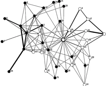
Fig. 1.Carbon ﬂow network of Chesapeake Bay in summer (arrow thickness pro-portional to ﬂux in mg C m−2_yr−1_{) from}_{Baird and Ulanowicz (1989), with black} nodes indicating pelagic compartments and white nodes indicating benthic com-partments. SeeTable 1for compartment codes.

prey, but do not choose other nodes to consume. We assumed that the non-living compartments [dissolved organic carbon (34), sus-pended particulate organic carbon (35) and sediment particulate organic carbon (36)] all could function as a kind of predator, in that they receive carbon in this model, just a as a predator would.

3. Results

3.1. Spring-embedder visualizations

We visualize the networks in their original form as described byBaird and Ulanowicz (1989). There was greatest diversity (36 compartments) and system complexity during the summer in

Fig. 2.Carbon ﬂow network of Chesapeake Bay in winter (arrow thickness proportional to ﬂux in mg C m−2_yr−1_{) fromBaird and Ulanowicz (1989), with black nodes indicating} pelagic compartments and white nodes indicating benthic compartments. SeeTable 1for compartment codes.

(6)

Table 2

Descriptive statistics for food web transitions in Chesapeake Bay.

Spring Summer Fall Winter

Mean degree 2.86 3.03 2.83 2.42

Number of new links created in next season

13 6 6 −

Number of new links terminated in next season 7 13 21 − Reciprocal links (mutualisms) 4 4 5 6 Indegree variance 6.0 7.0 6.4 6.8 Transitivity index 0.27 0.30 0.31 0.40

Chesapeake Bay and this is reflected in the visual display (Fig. 1). In this diagram, black nodes represent the plankton and pelagic species, and the white nodes show benthic groups. Most of the car-bon is flowing through the plankton and pelagic nodes at the left side of the plot (node 35 is suspended POC, which is linked directly to node 1 phytoplankton and node 7 ciliates, which themselves are linked because ciliates eat the phytoplankton, indirectly linked to node 6, flagellates). Lesser amounts of carbon are flowing in the benthos (node 36 is sediment POC), but there is a concentration of nodes and outdegree on these nodes is large. These are the two major nodes through which most carbon passes in the summer, the most active and connected one in the water column. Sediment POC (36) is detritus, and many arrows point there, tracing the flow of carbon as they die, hence the central position in spring-embedder. The increased organization of the system is evident when com-paring the summer plot (Fig. 1) with the winter spring-embedder (Fig. 2). There are fewer nodes [28 nodes, eight species are absent in winter, as shown in the upper right ofFig. 2, the unconnected nodes: (10) sea nettle, (20) fish larvae, (24) American shad, (27) spot, (30) bluefish, (31) weakfish, (32) summer flounder, and (33) striped bass], which have migrated from the system or died. Most of their carbon has flowed to the benthos, and most of these were pelagic during the summer (black nodes)]. The system in winter appears to be less complex and more focused around the detritus node (36) which is linked directly to the sediment bacteria (3) and other benthic predators.

3.2. SIENA continuous-time Markov chain model results

Table 2gives descriptive statistics of the food web network of Chesapeake Bay for each season. The mean degree was highest in summer (2.83 links per node), and lowest in winter (2.42 links per node). During the transition from spring to summer, more links were created than deleted (13 new links were created in summer, and 7 links were lost), while the converse was true for the transi-tions from summer to fall (6 links were created in fall, and 13 were lost) and fall to winter (6 links created in winter, but with 21 links lost). Together, these results suggest that the network became most complex in the summer and simpliﬁed in the winter. The total num-ber of reciprocal links varied from 4 to 6, and these are normally important in social networks, for example friendship. However, in

ecological systems, these represent mutualisms, and in Chesapeake Bay there are mutual connections between the non-living sedi-ment POC and some species like blue crabs, ciliates and zooplankton (detritivory).

The variance of indegrees (number of predators for each com-partment) was between 6 and 7, clearly higher than the mean degree (which would be expected for a Poisson distribution, implied by a random network). The transitivity index is deﬁned as the observed number of transitive triplets (ordered triplesi,j,hwhere

ieatsj,jeatsh, andieatsh) divided by possible number of transi-tive triplets (ordered triplesi,j,hwhereieatsjandjeatsh). The transitivity index increases from 0.27 for spring to 0.31 for fall and then increases sharply to 0.40 for winter.

Results of parameter estimation are shown inTable 3. The SIENA model was run separately for each seasonal transition (spring to summer, summer to fall, and fall to winter) and for all four seasons together (all seasons). Convergence of the model algorithm was excellent for all models. The rate parameter is the expected num-ber of opportunities for changes per predator compartment, and is a necessary ingredient of the model but less important for inter-pretation. The outdegree (prey link density) parameter is required to ﬁt the balance between the number of created and deleted links. The parameters are on the log-odds scale: an outdegree parameter of 0 would mean (if all other weight parameters likewise were 0) that, when comparing two pairs (i,j) where there is no tie fromito

j(idoes not prey onj) and (h,k) where there is a tie fromhtok(h

does prey onk), the probability of creating a new tie fromitojis just as large as the probability of terminating the tie fromhtok. Given that each species has only a limited number of other species that it preys upon, i.e., there are many more non-ties than ties, this would mean a sharp increase in the number of ties, which is unrealistic. In line with this, the estimated outdegree parameters are nega-tive, indicating that predators are in fact selective. The outdegree parameters also become more strongly negative over the seasons, reﬂecting that whereas more ties are created than terminated when going from spring to summer, relatively more and more ties are terminated when going toward Fall and especially Winter. In two of the transitions [spring–summer (−2.1805,z=−3.795,p< 0.001) and summer–fall (₋2.8713,z=₋3.632,p< 0.001)] and over all sea-sons (−3.264,z=−5.607,p< 0.001), the predators show signiﬁcantly negative outdegree parameter weights.

The weight of indegree popularity, the tendency for predator compartments to prey on those compartments that already have many predators, was signiﬁcantly positive in the spring–summer transition (ˇk= 0.1816, z= 1.914, p< 0.05), but not for the

summer–fall transition (ˇk= 0.1104, z= 0.865, p> 0.10) or the

fall–winter transition (ˇk= 0.6027, z= 0.982, p> 0.10). However,

the indegree popularity weightˇk= 0.1888 is signiﬁcantly positive

when compared across all seasons (z= 2.198,p< 0.05,Table 3). Thus over all seasons, and especially in the spring–summer transition, there is a tendency for prey that are already highly popular with predators to be selected by predators.

Finally, the transitive triples effect is an indication of how many clusters of three-compartments are interacting in the ecosystem. This effect measures the closure of a network, because when

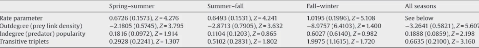
Table 3

SIENA Model parameter and effect estimates and standard errors (in parentheses) for each period of seasonal change. AZ-score is obtained by dividing the effect estimates by the standard error.

Spring–summer Summer–fall Fall–winter All seasons

Rate parameter 0.6726 (0.1573),Z= 4.276 0.6493 (0.1531),Z= 4.241 1.0195 (0.1996),Z= 5.108 See below

Outdegree (prey link density) −2.1805 (0.5745),Z= 3.795 −2.8713 (0.7905),Z= 3.632 −8.9757 (6.4103),Z= 1.400 −3.2641 (0.5821),Z= 5.607 Indegree (predator) popularity 0.1816 (0.0972),Z= 1.914 0.1104 (0.1203),Z= 0.865 0.6027 (0.6140),Z= 0.982 0.1888 (0.0859),Z= 2.198 Transitive triplets 0.2928 (0.2241),Z= 1.307 0.5102 (0.2831),Z= 1.802 1.9975 (1.1615),Z= 1.720 0.6635 (0.2100),Z= 3.160 Rate parameters in all seasons analysis: rate parameter spring–summer 0.6906 (0.1520). Rate parameter summer–fall 0.6472 (0.1457). Rate parameter fall–winter 0.9767 (0.1935).

(7)

predator iis feeding fromjand h, andjis also feeding onh, it suggests a closed interaction around these nodes. It is associated with omnivory in lower trophic levels. Low weights for transitive triples would be found in linear chain-like relations in the food web network; high weights are associated with clusters of nodes that are heavily interconnected. As the number of observed tran-sitive triples increases relative to the number that are possible (transitivity index), the network can be thought of as becom-ing more closed, or dependent on internal cyclbecom-ing of carbon. An increase in transitive triplets would be indicated by a positive weight associated with a significantp-value. In the Chesapeake Bay data, the weight of transitive triplets is positive but non-significant for the spring–summer (_ˇ_k= 0.2928,z= 1.307,p< 0.10). However, the transitive triples weight is increased and significant for the summer–fall transition (ˇk= 0.5102,z= 1.802,p< 0.05) and much greater in the fall–winter transition, which is also signif-icant in spite of the higher standard error (ˇk= 1.9975, z= 1.72, p< 0.05). When computed over all seasons, this effect was highly significant (ˇk= 0.6635,z= 3.160,p< 0.001). Taken together, these results on transitive triples suggest that the network was rela-tively open in spring through summer transition, because it was expanding as new species immigrated or re-appeared from win-ter hibernation, but became more closed from summer through winter as primary production of organic carbon decreased and compartments out-migrated, went into hibernation or locally extinct.

4. Discussion

We visualized the Chesapeake Bay trophic network using the published carbon flow data (Baird and Ulanowicz, 1989) and observed a dramatic change in the network’s structure as well as shifts in the carbon flows. Based on visual inspection of the network diagrams, the carbon flows during summer were dom-inant in the pelagic zone and interconnected with benthic sinks (sediment POC), while during the winter dominant flows were asso-ciated with the benthos. We used a statistical method devised for social network analysis to assess seasonal changes in trophic net-work structure (SIENA continuous-time Markov chain model). This method allowed a mathematically precise way to look at the struc-tural dynamics of the system, by comparing the observed structure at each season with Monte-Carlo simulations of the network struc-ture during transitions between seasons and across all four seasons. Network topology changed significantly during the transition from spring to summer, becoming more complex initially, then increas-ingly less complex during the transitions from summer to fall, and fall to winter. There was a net increase in the number of new links from spring to summer, but a net decrease in subsequent seasons. Network density and mean degree (links per node) declined from summer to winter along with the number of nodes. The transitivity index (a measure of network closure) increased from summer to winter.

These changes in network structure were largely in agreement with the observations ofBaird and Ulanowicz (1989)that the sys-tem was becoming more organized (ascendent) in the winter, with a lower system throughput. However, we do not agree with the conclusion of Baird and Ulanowicz (1989)that the Chesapeake ecosystem “. . .maintains essentially the same topological struc-ture throughout the cycle of seasons”. In fact, we conclude just the opposite, that the structure of the ecosystem network changes signiﬁcantly during the summer to winter transition, becoming signiﬁcantly more closed (as indicated by the increasingly posi-tive transiposi-tive triples), less chain-like and more interconnected. We conclude that this seasonal trend toward network closure is sta-tistically non-random, and that the Chesapeake ecosystem shows signs of increased organization around fewer nodes and increased

Table 4

A comparison of the normalized ascendency (Baird and Ulanowicz, 1989) and the transitivity index (number of transitive triples divided by the number of possible transitive triples) of the four seasonal networks in Chesapeake Bay.

Ascendency Transitivity index

Spring 0.626 0.27

Summer 0.615 0.30

Fall 0.646 0.31

Winter 0.666 0.40

efﬁciency as energy available from primary production declines in the winter.

The statistical analysis of the Chesapeake’s structural data also found changes that would reflect aspects of ascendency, in that the network structure became more clustered and closed from sum-mer to winter, which is another way of saying that it became more organized. Ascendency is a concept based on energy throughput and average mutual information (AMI flow diversity) and is asso-ciated with system organization and development (Ulanowicz and Robert, 2001). Our structural measures that best correlated with the normalized ascendency (corrected for throughput differences in the different seasons) patterns described by Ulanowicz and Baird (1989) are the transitive triples effect and the transitivity index (the number of transitive triples scaled as a fraction of the poten-tial number of transitive triples). Transitivity increased in winter, just as did normalized ascendency (correlation between transitivity index and ascendency = 0.85;Table 4). The increase in the transi-tivity index from summer through winter suggests that the food web trophic levels should be more compressed in the winter than the summer, because the transitive triples mostly involve the detri-tal compartments (Fig. 2).Baird and Ulanowicz (1989)also noted that the Chesapeake Bay’s trophic transfer efficiency declined at the highest trophic levels in winter. In fact, the ciliates and blue crabs, which are involved in the transfer of energy to the highest trophic levels the network, are responsible for more of the pro-duction reaching the fifth trophic level in the summer, whereas in winter little production reaches that level. In winter the greatest level reached is trophic level four. This decreased production that reached the fifth trophic level in the winter was correlated with the high transitivity index and large weight of transitive triplets. Both of these transitivity measures increased in the winter, whichBaird and Ulanowicz (1989)observed was responsible for the compres-sion of the trophic levels in that season, due to changes in structure and carbon flow as ciliates and blue crabs became more dependent on sediment POC and less on primary production from the plankton in the winter.

It should be noted that we did not assume any particular niche from which to draw prey at random or constrain the diet for any species, other than specifying that producers could not have prey. Therefore, in our simulations, consumer groups were allowed to feed on any of the other species at random. This decision to preda-tors to consume any prey is a bit broad; e.g., striped bass can potentially consume phytoplankton in some of the null models used for statistical comparison. However, it is important to realize that the SIENA model permits speciﬁcation of “structural zeros”, which forbid particular ordered pairs of nodes from interacting, as well as “structural ones”, which require particular pairs to interact. In this introductory analysis, we used these options only in a lim-ited way, namely to forbid primary producer compartments from having prey. In future simulations, we could use this model fea-ture to specify which links must always occur or could never occur. Clearly, this approach differs from the niche model (Williams and Martinez, 2000), the cascade model (Cohen and Newman, 1985) and the phylogenetic constraint (Cattin et al., 2004) model, which impose additional constraints on which nodes can be connected in dynamic simulations using ecological niche axes, trophic levels, or

(8)

phylogenies. We feel the SIENA approach is an important contri-bution in that it does not assume any kind of a niche axis or other constraint when nodes are allowed to change their link distribu-tion over time, although, clearly, some restricdistribu-tions must be made for producers.

Like other dynamic models, the continuous-time Markov chain model in SIENA is based on a binary matrix of node interactions, and not carbon or energy flow. There is a need to explore the appli-cation of this approach for both carbon flows and predator/prey data, including the ability to handle valued data of different forms (e.g., carbon, percent of diet). The developers of SIENA are currently working on extensions of the model to valued data. However, the issue is more complex than binary versus valued data. An important consideration is the fit between the different types of ecological net-work and food web data and the assumptions of the SIENA model with respect to nodes making choices that create or delete network links. Flows and predation reflect different aspects of the ability of network actors (e.g., compartments in a food web) to initiate choices. BothPatten (1981, 1982)andFath (2004)have discussed how both the receivers and generators of transactions in ecological networks have dual roles, in that both have control and influence over the maintenance of the configuration of an ecosystem’s overall flow storage. These controls, both up and down the system, need to be considered more closely in future applications and alterations of the model.

An important advantage of the SIENA modeling approach we have presented here is that it not only provides indications of the amount of change in a network, but provides a formal way to specify the kinds of structural changes that have occurred. This is accom-plished via the speciﬁcation of various types of subgraphs or motifs that the model parameterizes. Further, the application of a statis-tical model allows (a) the measurement of change parameters for each kind of micro-structure, such as transitivity, while simulta-neously controlling for other changes, and (b) permits signiﬁcance tests on food web statistics. The most recent versions of the model also permit using multiple relations (such as non-trophic interac-tions) as covariates, in addition to taking account of both constant and variable attributes of network nodes.

In the future, the model can be made even more useful by iden-tifying and incorporating structural effects that are more central to ecological network theory and analysis, particularly those that are important for understanding ecosystem dynamics. This is a promis-ing area of research, particularly as longitudinal ecological network data sets become more available. We end by suggesting that this approach could help in answering some of the vexing questions relevant to recent interests in complexity and adaptive food web architecture.

4.1. A concluding observation on economic and ecological networks

Given that we have used a model developed in the social sci-ences to illuminate ecological data, it is interesting to speculate on the similarity of the seasonal changes in the Chesapeake’s trophic network and the current condition of US and global economic net-works. Summer in Chesapeake Bay is like the US economy during the period of 1990–2008; energy, credit and capital were unlim-ited or at least being produced much faster than they were being consumed. However, the US’s, and indeed the world’s, economic network is now entering the economic equivalent of the Chesa-peake Bay’s winter: a slow-down of available energy (declines in productivity of oil, associated with the Iraq war or simply the “End of Oil” phenomenon), loss of credit and capital, and the resulting loss of the economic nodes (bankrupting of businesses, increased unemployment, downsizing of work staff, including jobs being lost at our own university). These changes, however, can lead to

increased energy efficiency and improve organizational structure of the ecosystem and the economy, especially as the ecological or economic network shrivels and simplifies. Natural selection will preserve the most energetically or metabolically efficient nodes after the period of reduced resources at the producer level. Whether or not the global economy will recover as the Chesapeake’s trophic network does each new spring remains to be observed.

References

Allesina, S., Alonso, D., Pascual, M., 2008. A general model for food web structure. Science 320 (5876), 658–661.

Baird, D., Ulanowicz, R.E., 1989. Seasonal dynamics of the Chesapeake Bay ecosystem. Ecol. Monogr. 59, 329–364.

Baird, D., Heymans, J.J., 1996. Assessment of the ecosystem changes in response to freshwater inﬂow of the Kromme River Estuary, St. Francis Bay, South Africa: a network analysis approach. Water SA 22, 207–318.

Baird, D., Luczkovich, J., Christian, R.R., 1998. Assessment of spatial and temporal variability in ecosystem attributes of the St. Marks National Wildlife Refuge, Apalachee Bay, Florida. Estuar. Coast. Shelf Sci. 47, 329–349.

Belgrano, A., Scharler, U.M., Dunne, J., Ulanowicz, R.E., 2005. Aquatic Food Webs: An Ecosystem Approach. Oxford University Press, Oxford, UK, p. 262.

Borgatti, S.P., 2002. NetDraw: Graph Visualization Software. Analytic Technologies, Harvard.

Buss, L.W., Jackson, J.B.C., 1979. Competitive networks: nontransitive competitive relationships in cryptic coral reef environments. Am. Nat. 113, 2–223. Cattin, M.F., Bersier, L.F., Banasek-Richter, C., Baltensperger, R., Gabriel, J.P., 2004.

Phylogenetic constraints and adaptation explain food-web structure. Nature 427 (6977), 835–839.

Cohen, J.E., Newman, C.M., 1985. A stochastic theory of community food webs. I. Models and aggregated data. Proc. R. Soc. Lond. Ser. B 224, 421–448. de Ruiter, P., Wolters, V., Moore, J. (Eds.), 2005. Dynamic Food Webs: Multispecies

Assemblages, Ecosystem Development and Environmental Change. Elsevier, Amsterdam, The Netherlands, p. 590.

Dell, A.I., Kokkoris, G.D., Banasek-Richter, C., Bersier, L., Dunne, J.A., Kondoh, M., Romanuk, T.N., Martinez, N.D., 2005. How do complex food webs persist in nature? In: de Ruiter, P., Wolters, V., Moore, J. (Eds.), Dynamic Food Webs: Multispecies Assemblages, Ecosystem Development and Environmental Change. Elsevier, Amsterdam, The Netherlands, p. 590.

Dunne, J., Brose, U., Williams, R.J., Martinez, N.D., 2005. Modeling food-web dynam-ics: complexity–stability implications. In: Belgrano, A., Scharler, U.M., Dunne, J., Ulanowicz, R.E. (Eds.), Aquatic Food Webs: An Ecosystem Approach. Oxford University Press, Oxford, UK, pp. 117–128.

Eades, P., 1984. A heuristic for graph drawing. Congressus Numerantium 42, 149–160. Fath, B.D., 2004. Distributed control in ecological networks. Ecol. Model. 179,

235–245.

Gajer, P., Kobourov, S.G., 2002. GRIP: Graph drawing with intelligent placement. J. Graph Algorithms Appl. 6 (3), 203–224.

Heymans, J.J., Christensen, V., Guénette, S., Christensen, V., 2007. Evaluating network analysis indicators of ecosystem status in the Gulf of Alaska. Ecosystems 10 (3), 488–502.

Huisman, M., Snijders, T.A.B., 2003. Statistical analysis of longitudinal network data with changing composition. Sociol. Methods Res. 32, 253–287.

Li, B., Charnov, E.L., 2001. Diversity–stability relationships revisited: scaling rules for biological communities near equilibrium. Ecol. Model. 140, 247–254. McCann, K., Rasnussen, J., Umbanhowar, J., Humphries, M., 2005. The role of space

time and variability in food web dynamics. In: de Ruiter, P., Wolters, V., Moore, J. (Eds.), Dynamic Food Webs: Multispecies Assemblages, Ecosystem Development and Environmental Change. Elsevier, Amsterdam, The Netherlands, pp. 56–70. Mollet, H.F., Cailliet, G.M., 2002. Comparative population demography of

elasmo-branchs using life history tables, Leslie matrices and stage-based matrix models. Mar. Freshwater Res. 53, 503–515.

Pascual, M., Dunne, J.A. (Eds.), 2006. Ecological Networks: Linking Structure to Dynamics in Food Webs. Oxford University Press, New York.

Patten, B.C., 1981. Environs: the superniches of ecosystems. Am. Zool. 21, 845–852. Patten, B.C., 1982. Environs: relativistic elementary particles or ecology. Am. Nat.

119, 179–219.

Polis, G.A., Winemiller, K.O. (Eds.), 1996. Food Webs: Integration of Patterns and Dynamics. Chapman and Hall, New York.

Scharler, U.M., Baird, D., 2005. A comparison of selected ecosystem attributes of three South African estuaries with different freshwater inﬂow regimes, using network analysis. J. Marine Syst. 56 (3–4), 283–308.

Snijders, T.A.B., 2001. The statistical evaluation of social network dynamics. In: Sobel, M.E., Becker, M.P. (Eds.), Sociological Methodology-2001. Basil Blackwell, Boston and London, pp. 361–395.

Snijders, T.A.B., Steglich, C.E.G., Schweinberger, M., Huisman, M., 2007. Manual for SIENA Version 3. University of Groningen, ICS/University of Oxford, Department of Statistics, Groningen/Oxford, http://stat.gamma.rug.nl/stocnet.

Ulanowicz, Robert, E., 2001. Information Theory in Ecology. Comput. Chem. 25, 393–399.

Williams, R.J., Martinez, N.D., 2000. Simple rules yield complex food webs. Nature 404, 180–183.

Wootton, J.T., 2001. Prediction in complex communities: analysis of empirically derived Markov models. Ecology 82 (2), 580–598.