Process Scheduling in DSC and the Large Sparse Linear Systems Challenge*

Process Scheduling in DSC and the Large

Sparse Linear Systems Challenge*

A. Diaz, M. Hitz, E. Kaltofen, A. Lobo and T. Valente**

Troy, NY 12189-3590, USA

Internet: diaza, hitzm, kaltofen, [email protected]; [email protected]

Abstract. _{New features of our DSC system for distributing a symbolic} com-putation task over a network of processors are described. A new scheduler sends parallel subtasks to those compute nodes that are best suited in han-dling the added load of CPU usage and memory. Furthermore, a subtask can communicate back to the process that spawned it by a co-routine style calling mechanism. Two large experiments are described in this improved setting. We have implemented an algorithm that can prove a number of more than 1,000 decimal digits prime in about 2 months elapsed time on some 20 com-puters. A parallel version of a sparse linear system solver is used to compute the solution of sparse linear systems over finite fields. We are able to find the solution of a 100,000 by 100,000 linear system with about 10.3 million non-zero entries over the Galois field with 2 elements using 3 computers in about 54 hours CPU time.

1 Introduction

In Diaz et al. (1991) we introduced our DSC system for distributing large scale symbolic computations over a network of UNIX computers. There we discuss in detail the following features:

— The distribution of so-called parallel subtasks is performed in the applica-tion program by a DSC user library call. A daemon process, which has established IP/TCP/UDP connections to equivalent daemon processes on the participating compute nodes, handles the call and sends the subtask to one of them. Similarly, the control flow of the application program is syn-chronized by library calls that wait for the completion of one or all subtasks. — DSC distributes not only remote procedure calls to precompiled programs, but also programs that are first compiled on the machine serving the sub-task. This enables the distribution of dynamically generated “black-box” *This material is based on work supported in part by the National Science Foun-dation under Grant No. CCR-90-06077, 91-21465, and under Grant No. CDA-88-05910.

**Valente’s current address is Department of Mathematics and Computer Science, Colby College, Waterville, Maine 04901.

functions (cf. Kaltofen and Trager 1990) and easy use of computers of dif-ferent architecture.

— DSC can be invoked from both Common Lisp and C programs. It can distribute within a local area network (LAN) and across the Internet. — The interface to the application program consists of seven library functions.

Processor allocation and interprocess communication is completely hidden from the user.

— The progress of a distributed computation can be monitored by an inde-pendently run controller program. This controller also initializes the DSC environment by establishing server daemons on the participating computers. — We document experiments with DSC on a parallel version of the Can-tor/Zassenhaus polynomial factorization algorithm and the Goldwasser-Kilian/Atkin (GKA) integer primality test.

New experiments with the GKA primality test that run on so-called “ti-tanic” integers, i.e., integers with more than 1000 decimal digits, and experi-ments with a parallel sparse linear system solver, namely, Coppersmith’s block Wiedemann algorithm (Coppersmith 1992), have lead to several key modifica-tions to DSC. In this article we describe these changes, as well as the results obtained by applying the improved environment to both titanic primality test-ing and sparse linear system solvtest-ing.

Unlike on a massively parallel computer, where each processor has the same computing power and internal memory, a network of workstations and machines is a diverse computing environment. At the time the application program dis-tributes a subtask, the DSC server has to determine which machine will receive this subtask. Our original design used a round-robin schedule, which resulted in quite bad subtask-to-processor allocation. The new scheduler continuously receives the CPU load and memory usage of all participating machines, which are probed by resident daemon processes at 10 minute intervals. In addition, the application program supplies an estimate of the amount of memory and a rough measure of CPU usage. The scheduler then makes a sophisticated selection of which processor is to handle the subtask. If certain threshold values are not met, the subtask gets queued for later distribution under hopefully better load con-ditions on the network. The details of the scheduling algorithm are described in

§2.1. Without this very fine tuned distribution scheduler, neither the primality tester nor the sparse linear system solver could have been run on as large inputs as the ones we had. Note that DSC’s ability to account for the heterogeneity of the compute nodes is one distinguishing mark to other parallel computer algebra systems such as Maple/Linda (Char 1990), PARSAC-2 (Collins et al. 1990), the distributed SAC-2 of Seitz (1992), or PACLIB (Hong and Schreiner 1993).

DSC supports a very coarse grain parallelism. This was quite successful for the primality tester, where each parallel subtask is extremely compute intensive but uses a moderate amount of memory. However, the Wiedemann sparse linear system solver can be implemented by slicing the coefficient matrix and storing each slice on a different processor. These slices will repeatedly be multiplied by

a sequence of vectors. We have implemented a mechanism whereby the subtasks remain loaded in memory (or swap space) on first return, and can be continued at the point following the previous return with different data supplied by the calling program, much like co-routines (see _§2.3). This introduces a finer grain parallelism and allows two-way communication between the subtask and the parent process. This co-routine mechanism tends to make use of the distributed memory more than the parallel compute power.

DSC has also been modified internally in two important ways. First, the environment can now be initialized on a user supplied UDP port number. Sev-eral users can thus set up individual DSC servers without interfering with one another. We note that the inter-process communication does not take place on the system level, where a single port number could have been reserved for DSC. Hence no system modifications are necessary to run DSC, which is often desired when linking to off-site computers. Nonetheless, the port number is public and servers could be started, perhaps maliciously, to communicate with an existing environment. We guard against such mishap by tagging each message with a key set by the individual user. More details on these enhancements are found in

§2.2.

Our first test problem has been the GKA primality test applied to numbers with more the 1000 decimal digits. We are successful in proving the primality of a 1111 digit number on a LAN of some 20 computers in about 2 months turnaround time. The details and observations of this experiment are described in _§2.4. Our second test problem is a distributed version of the Coppersmith block Wiedemann algorithm. This algorithm for solving unstructured sparse lin-ear systems has very coarse grain size, unlike classical methods such as conjugate gradient, which makes it very suitable for the DSC environment. We have imple-mented two variants, one for entries being from prime finite fields whose elements fit into 16 bits, and one for entries from GF(2), the field with two elements. In the latter case, we not only realize Coppersmith’s processor internal parallelism by performing the bit operations simultaneously on 32 elements stored in a sin-gle computer word, but we further “doubly” block the method and distribute across the network. The details of our experiments are described in _§3; we are successful in speeding up the solution of 100,000_×100,000 linear systems with 10.3 million entries over GF(2) by factors of 3 and more. Such large runs would very likely not have completed using our old round-robin scheduling, since only the selection of compute nodes with large memory makes our programs feasible.

2. New DSC Features

2.1 The DSC Scheduler

The goal of process scheduling in DSC is to locate available resources in the network and to distribute subtasks without creating peak loads on any node. Selection of a suitable computer is based on three factors:

Load on nodes Rating of resources Requirements for subtask – Long term – MIPS of processors – crude estimates by user – Most recent – Installed memory

The hardware resources are defined in three fields of the node list: the core memory size in MByte, the CPU power in MIPS and the number of processors. In the application program the user has to specify an estimate for the expected memory needs in MByte and a “fuzzy” value (LOW, MEDIUM, HIGH) for CPU usage.

In order to provide the scheduler with information about the current and the expected load at each compute node, a method of data collection had to be developed. The ideal load-meter would provide exact data in real time with some corrections derived from trend predictions. This would require the monitoring program being tied to the operating system on a low level. Unfortunately this would place excessive burden on the user (request for higher privileges) and it would make the system less portable. However, most of the time it is not desirable to have measurements with high resolution. The readings should reflect trends for longer time periods rather than being just snapshots. As a first solution the UNIXpscommand was chosen to measure CPU and memory usage about 8 to 10 times an hour. Due to the latency (up to one minute) involved with ps, and for better modularity, a separate process “DSC_ps” was added in the current version of DSC.

Once a DSC server is running, it spawns off the DSC_ps process for its node. DSC_ps maintains a table of statistics, which is saved to disk after each update.

At the end of the hour, the mean of CPU and memory usage is averaged with the previous value for this hour of the day. At the end of the day (or week) the values for this day of the week (or week of the year) are adjusted by the latest readings. From all four levels (current reading, hour, day and week) a weighted average is computed to include long term effects. The resulting two values (CPU, memory) are sent to the local DSC server which in turn will communicate the update to all other servers on the network. The backup file allows the initialization of load parameters according to anticipated patterns of usage. DSC_ps will then adapt

those guessed values with respect to the new readings.

The scheduler in the DSC server uses the values received from DSC_ps, the ratings from the node database, and the estimated needs of the next task to select the target machine. For this purpose a sorted list of compute nodes which satisfy a minimum requirement of available memory is maintained. Based on the memory estimate of the application, all nodes which would stay above a certain threshold (allowing for some moderate paging) are preselected. Among them the one with the lowest CPU usage is finally chosen for distribution. If none of the nodes can satisfy the requirements, the job is put back into a queue until the load on one of the computers decreases to a sufficient level.

After distributing the new task the server adjusts for the expected change in the load parameters of the selected node. Because of the long latency period, it cannot wait for the next readings of the actual load when it has to distribute many tasks in a short period of time. In time it can replace the estimates by the actual values whenever new load readings are received from the other server. This has the convenient side effect that the distributing server does not have to rely on transient measurements resulting from the startup phase of the new task

(which can involve compilation of source code). Most of the time it will receive the steady-state readings because the server of the selected compute nodes will send the update of the load parameters with low priority.

2.2 Interprocess Communication and Message Validation

DSC uses the User Datagram Protocol (UDP) for most of its communication and Transmission Control Protocol (TCP) stream sockets for file transfer. For the sake of portability, all inter-process communication adheres to the DARPA Inter-net standard TCP/IP/UDP as implemented in UNIX 4.2/4.3bsd (see Diaz 1992). This low level approach avoids the high latency present in the UNIX rsh and

ftp commands, and it provides real time information on subtasks and compute

nodes for possible control actions such as subtask rescheduling. Before a user starts an application program that distributes parallel subtasks over the network, the DSC server daemons must be started. These daemon programs execute in the background and monitor a single UDP datagram address for new external stimuli from other DSC servers, the DSC controller program, the resource and work load monitor daemon program DSC_ps, and application programs. In or-der for a client process to contact a DSC server, the client must have a way of identifying the DSC server it wants. This can be accomplished by knowing the 32-bit Internet address of the host on which the server resides and the 16-bit port number which identifies the destination of the datagram on the host ma-chine. Each DSC server must be using the same UDP port number in order to communicate with the others. UDP port numbers are not reserved and can be allocated by any process. The run time port number allocation option allows the user to automatically poll the machines in the configured DSC network to find a suitable port number for the initiation of a set of DSC servers. This is done via the DSC control program and consequently all DSC servers can be started using the determined available port number for their UDP communication.

If the control program could not establish a connection to a DSC server via the port number specified in the configuration file, the control program will assume that no active DSC server is monitoring this port. Consequently, the control program searches for an available port number which is not used on any machines in the “farm” of compute nodes in the DSC network. Optionally, the user may specify its own port number thereby bypassing the runtime port number allocation mechanism.

Once a port number has been determined the control program will start up the remote DSC servers via a rsh command supplying the executable and the port number to the remote or local compute node. Once all DSC servers are active communication takes place only via the IP/TCP/UDP protocols.

The primary function of the DSC server daemon program is to monitor a single UDP datagram address for incoming messages. Each message is a request for the DSC server to perform some action. However, in order to act only on messages received from the user that started the server, all messages contain a message validation tag which is specified by the user. If for any reason the message validation tag received by the DSC server does not match the server’s message validation tag, the message is ignored and the invalid action request

is logged. This avoids the inadvertent message passing that could occur when multiple DSC systems execute concurrently in the same open network computing environment using the same datagram port number.

2.3 Co-Routines

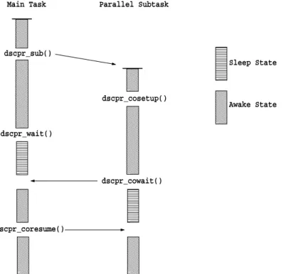
The C and Lisp DSC application programmer can take advantage of the re-sources found in the DSC network by utilizing 5 base functions callable from a user’s program. The function dscpr_sub is used for the activation of paral-lel subtasks and designating their respective resource usage specifications. The calls todscpr_wait,dscpr_next, anddscpr_killare used to wait on a specific parallel subtask or on the completion of all parallel subtasks, to wait for the next completed parallel subtask and to kill a specific parallel subtask, respectively. Finally, the function dscdbg_start can be used to track a task and is useful when one wishes to debug tasks using interactive debuggers such as Unix’sdbx.

Main Task dscpr_sub() dscpr_wait() dscpr_coresume() Parallel Subtask dscpr_cosetup() dscpr_cowait() Sleep State Awake State

Figure 1: Co-routine flow of control.

In order to meet the sparse linear system challenge (see_§4), where there is a need to maintain large amounts of data within parallel subtasks, the C User Li-brary has been extended to allow the user to implement co-routines (Kogge 1991,

§9.6.3). The functiondscpr_cosetupmust be called at the beginning of any par-allel subtask that is to be treated as a co-routine. This initialization is necessary so that the wake up signal received by a parallel subtask from the DSC server can be interpreted as a command to resume execution of the subproblem. Specif-ically, thedscpr_cosetupfunction specifies how the subtask process will handle an asynchronous software interrupt by providing the address of an internal DSC function that wakes the process from a sleep state when the corresponding in-terrupt signal is detected. When the subtask calls the dscpr_cowait function,

it enters a sleep state and optionally transmits a data file back to its parent. Once a co-routine parallel subtask or a set of co-routine parallel subtasks has been spawned by a call to dscpr_sub, the returned indices have been recorded, and a successful wait has completed, the parent task can send a wake up call to a sleeping parallel subtask via the dscpr_coresume function. Arguments to this function are an integer which uniquely identifies a parallel subtask (returned from the spawning call to dscpr_sub) and a string which identifies which input file if any should be sent to the co-routine before the parallel subtask is to be resumed. This call essentially generates the software interrupt needed for the waking of the sleeping parallel subtask. Figure 1 denotes the relationship that could exist between DSC utility function calls in a main task and its co-routine parallel subtask child.

2.4 The GKA Primality Test

In this section, we describe new experimental results with our distributed implementation of the Goldwasser-Kilian/Atkin (GKA) primality test, which uses elliptic curves to prove an integer p prime; for earlier results, see Kaltofen et al. 1989, Diaz et al. 1991. In particular, we discuss here our success in proving “titanic” integers, i.e., integers with more than 1000 decimal digits, prime (see also Valente 1992, Morain 1991).

Let us briefly summarize the algorithm. The test has two phases: in the first phase, a sequence _{pi} of probable primes is constructed, such that p =

p0 > p1 > p2 > · · · > pn. Each pi+1 is obtained from pi by first finding

a discriminant d such that pi splits as ππ in the ring of integers of the field

Q(√d). If (1₋π)(1₋π) is divisible by a sufficiently large (probable) prime q, we setpi+1 toq, thus “descending” frompi topi+1. We then repeat the process, seeking a descent from pi+1. The first phase terminates with pn having fewer

than 10 digits. In the second phase, it is necessary to construct, for eachpi from

the first phase, an appropriate elliptic curve over GF(pi) which is used to prove

pi prime, provided pi+1 is prime. This results in a chain of implications

pn prime =⇒pn−1 prime =⇒ · · ·=⇒p0 =p prime.

In our experiment, we started with a probable prime number of 1111 deci-mal digits. Our code is written in the C programming language calling the Pari library functions (Batut et al. 1991) for arbitrary precision integer arithmetic. Each time a descent is required in the first phase, a list of nearly 10,000 dis-criminants is examined. In fact, we chose to search all d with _|d_{| ≤} 100,000, where Q(√d) has class number _≤ 50. Unfortunately, when p is titanic, few if any of these discriminants will induce a descent. For our prime of 1111 digits, we distributed the search for a descent from pi to pi+1 to 24 subtasks, each of which is given approximately 400 discriminants to examine. The first subtask to find a descent reports it to the main task which then redistributes in order to find a descent from pi+1. We required 204 descents before a prime of 10 digits was obtained. Our first phase run with the 1111 digit number as input began on January 12, 1992, and ended on February 13, 1992. The total elapsed time for

0 200 400 600 800 1000 1200 0 100 200 300 400 500 600 DIGITS REMAINING

ELAPSED TIME (HOURS)

Figure 2: Graph of progress of GKA first phase.

the run was measured at about 569 hours, or approximately 31₂ weeks. Figure 2 depicts the progress of this run during this period.

Notice that after 135 elapsed hours, the 1111 digit number is “reduced” to a number having 1044 digits. After an additional 43 hours, it appears that we regress, because the number shown now has 1045 digits! In fact, what has happened is that our program failed to find a descent from the 1044 digit number, and was forced to backtrack to a larger prime and find an alternate descent. Slow but steady progress is evident, until the last day, when the 322 digit number rapidly shrinks, and the first phase suddenly ends. Interestingly, it appears that about half of the total elapsed time of this run is spent merely reducing the original number to subtitanic size.

For our second phase run with 1111 digit inputs, there are a total of 204 descents to process. Typically, each of the 20 or so workstations is given about 10 descents. For each descent, the subtask must construct a class equation for the class field over Q(√d), find a root of the class equation, then use this root to construct an elliptic curve over the appropriate prime field GF(p). Once this curve is found, verification proceeds by finding a point on the curve which serves as a witness to the primality of p. Difficulties arise when the root-finder must handle class equations of degree 30 or more. Since the second phase is so sensitive to the degree of the class equation, it is critical that in the first phase we do whatever is possible to insure that only discriminants of relatively low class numbers are passed on to the second phase. Because of these factors, our phase two run for this titanic input takes approximately three weeks elapsed time. In a situation like this where a distributed subtask has a long running

time it is much more difficult to schedule the task on a processor with expected low load, thus insuring high performance.

3 Distributed Sparse Linear System Solving

3.1 Introduction and Background Theory

We now discuss our experience with DSC in the solution of homogeneous systems of sparse linear equations. The problem is to find a non-zerowsuch thatBw = 0, where B is a matrix of very large order N. The classical method of Gaussian elimination is not well suited for this task as the memory and time complexity are bounded by functions that are quadratic and cubic, respectively, inN.

Wiedemann (1986) gives a Las Vegas randomized algorithm with time com-plexity governed by O(N) applications ofB to a vector plus O(N2) arithmetic operations in the field of entries. The algorithm does not alter the sparsity of the coefficient matrix and requires only a linear amount of extra storage. The al-gorithm yields a non-zero solution with high probability. Wiedemann also gives a similar method for non-singular systems, although one could easily transform the non-singular to the homogeneous case by the addition of an extra column.

Coppersmith (1992) presents a generalization of Wiedemann’s algorithm which can be implemented in a distributed setting. For the purposes of this paper we shall now give a brief description of it, which is outlined in Figure 3.

(0) Select random x, z such that xtr_{Bz has full rank;} y_←Bz;

comment: x, y, z are N _×n block vectors with random entries from the ground field. (1) L_{← b}2N/n_c+ 5;

for i= 0,1, . . . , L do

a(i)_{= (x}tr_Bi_y)tr_;

comment: the m_×n matrices a(i) _{are coefficients} of a polynomialA(λ) of degree L.

(2) Λ_← find_recurrence(A);

comment: Λ(λ) is obtained by the generalized, block Berlekamp/Massey algorithm.

(3) for l= 1, . . . , n do

wl← evaluate(Λ, B, z, l);

comment: This steps yields wl such that Bwl= 0

and hopefully wl6= 0.

Figure 3: Outline of the block Wiedemann algorithm.

In the initializing step (0), one generates block vectorsx andz with dimen-sions N _×m and N _×n whose entries are randomly chosen from the ground

field. The vectors meet the conditions that xtr_{Bz has full rank. In subsequent} discussions we shall take m = n and refer to n as the blocking factor of the algorithm.

Next, step (1) is the computation of L = _b2N/n_c+ 5 terms of a sequence whoseith term isa(i)_{= (x}tr_Bi_y)tr _{wherey =Bz. It is clear that the individual}

columns of a(i) _{can be computed independently and in parallel. To do this we} distribute the vectorx and theνth column ofyalong withB and collect theνth columns of a(i)_{. Each of the parallel subtasks involves no more than b2N/nc+} 5 multiplications of B by vectors (Kaltofen 1993). The original Wiedemann algorithm requires 2N such applications.

Step (2) is to find a polynomial Λ(λ) representing a linear recurrence that generates the sequence. In the original Wiedemann Algorithm, thea(i) _{are field} elements and their recurrence is obtained by the Berlekamp/Massey Algorithm. In the present context, the a(i) _{are n×n matrices and we have to use} Copper-smith’s generalization. The individual a(i) _{are treated as the coefficients of the} polynomialA(λ) =PL

j=0a(

j)_λj_{. We iteratively compute the matrix polynomial}

Fj(λ) = · Λj(λ) Ψj(λ) ¸ .

During each iteration 1 _≤ j _≤ L we also compute a discrepancy matrix ∆j,

which is the coefficient of λj _{in F}

j(λ)A(λ).

The firstnrows ofFj are analogous to a bank of “current” shift registers and

the lastnrows represent a “previous” bank, as in the original Berlekamp/Massey algorithm. The task at hand is to compute a non-singular linear transformation Tj that will zero out the first nrows of ∆j. Initially, the rows of Fare assigned

nominal degrees and in determining Tj, one selects a pivot row in ∆j

corre-sponding to a row of lowest nominal degree in Fj and uses it to zero out the

appropriate columns of ∆j. Completing the iterative step, Fj is updated by

set-ting Fj+1 = DTjFj, where D = diag[1, . . . ,1, λ, . . . , λ] increments the nominal

degrees of the last n rows by 1. Overall, the whole step requires O(nN2) field operations. At present this step is done sequentially.

In step (3) one obtains a vectorwl which is non-zero with high probability,

and which satisfies Bwl = 0. It involves a Horner-type evaluation at B of

a polynomial derived from Λ with coefficients that are N-dimensional vectors and, additionally,O(N2_{) arithmetic operations. This step requires no more than} N/n+ 2 multiplications of B by vectors. There are n options of finding vectors in the kernel of B, one for each 1_≤l _≤n. With high probability the solutions found are nontrivial, at least, if the field of entries is sufficiently large. For GF(2), hopefully, some of the solutions will be nontrivial. That these different solutions sample the entire null space can so far only be argued heuristically. For the details the reader is referred to (Coppersmith 1992 and Kaltofen 1993). Our implementation is in the C programming language on computers run-ning UNIX. The programs are written generically, mearun-ning that the underlying field of entries can be changed with very little difficulty. We have successfully used DSC to distribute the task outlined in step (1). The DSC scheduler was

given a list of approximately 30 machines of diverse processing power and mem-ory capacity and the processing and storage requirements of the subtasks. From this information it selected suitable target hosts.

3.2 The Generic Arithmetic Package

In our implementation we sought the ability to program the arithmetic oper-ations generically. This was accomplished by writing all the field arithmetic operations as macros and implementing the macros in a way specific to the un-derlying field. At the moment, arithmetic can be done in the fields GF(2k_{) and}

GF(p) where k can be from 1 to 31 and p is a prime requiring at most 15 bits for its binary representation. These restrictions come from the maximum size of a word in the target machines. The macro implementations and corresponding basic datatypes are selected by setting a single software switch at compile time. The actual programs require no changes.

For the GF(2k_{) case the binary operations are implemented using the bit}

operations ofexclusive-or,and, andshift available in the C language. Field divi-sion is done by computing the inverse of an element with the extended Euclidean algorithm inside of which division is done using bit operations. In GF(2), a single bit is sufficient to represent an element and hence the operations of addition and multiplication are exactly the bit-operations exclusive-or and and, respectively. In Coppersmith’s implementation, 32 bit vectors are packed into a single vector of machine words. Thus, on a single processor, 32 vectors can simultaneously be multiplied into a matrix with bit entries. We have used the same approach in a special implementation for GF(2). In addition, we do “double blocking” in step (1), where we distribute several packed vectors to different compute nodes. For the field GF(p) the binary operations are implemented with built-in in-teger arithmetic operations. The limit of 15 bits keeps any intermediate product of two members of the field from overflowing the bounds of an unsigned 31-bit integer. The maximum permitted value ofp is thus 215_{−19 = 32749.}

3.3 Experimental Results and Observations

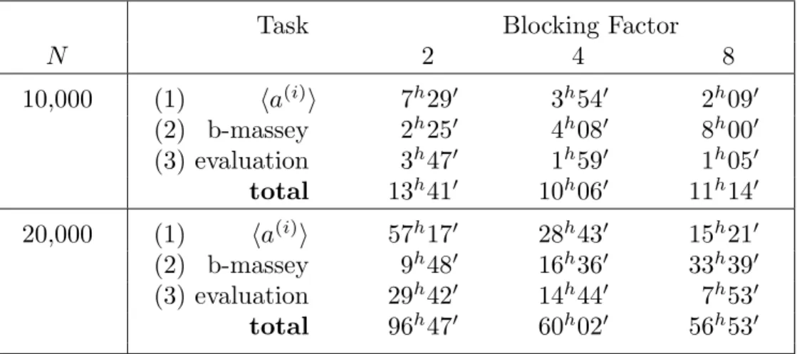
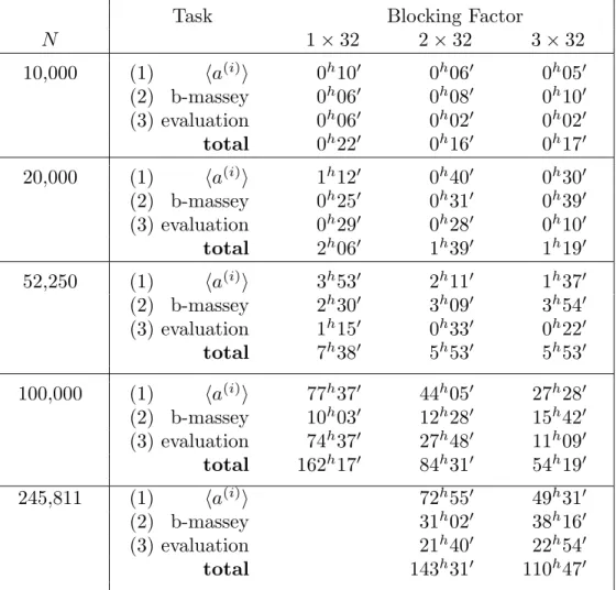
We conducted tests in the field GF(32749) using sparse square matrices with row dimensions of 10,000 and 20,000, and in the field GF(2) with dimensions 10,000, 20,000, 52,250, and 100,000 respectively. In the case of dimension 10,000 there are between 23 and 47 non-zero elements per row and approximately 350,000 non-zero entries in total; in the case of dimension 20,000, 57 to 73 non-zero ele-ments per row and 1.3 million non-zero entries in total. In the case of dimension 52,250 there are between 9 and 34 non-zero elements per row and altogether 1.1 million non-zero entries. The largest matrix contained 89 to 117 entries per row and a total of 10.3 million entries. The matrix of dimension 52,250, aris-ing from integer factoraris-ing by the MPQS method, was supplied to us by A. M. Odlyzko, while the other matrices were generated with randomly placed random non-zero entries. The tests were done with blocking factors of 2, 4, and 8 in the GF(32749) case and 32, 64, and 96 in GF(2). The calculation of the sequence

ha(i)_{i was done in a distributed fashion using DSC. Pointers to the matrix and} the vectorsx and yν were sent out to separate machines and the corresponding

components of A were returned. The computation of the generator polynomial and the evaluation of the solution were done on a single SUN-4 machine rated at 28.5 MIPS. Compilation was done with the optimizer flag activated. Figures 4 and 5 below give the actual CPU time taken for each task. The evaluation time is the time to find the first non-zero solution.

Task Blocking Factor

N 2 4 8 10,000 (1) _ha(i)_{i 7}h₂₉0 ₃h₅₄0 ₂h₀₉0 (2) b-massey 2h₂₅0 ₄h₀₈0 ₈h₀₀0 (3) evaluation 3h₄₇0 ₁h₅₉0 ₁h₀₅0 total 13h₄₁0 ₁₀h₀₆0 ₁₁h₁₄0 20,000 (1) _ha(i)_{i 57}h₁₇0 ₂₈h₄₃0 ₁₅h₂₁0 (2) b-massey 9h₄₈0 ₁₆h₃₆0 ₃₃h₃₉0 (3) evaluation 29h₄₂0 ₁₄h₄₄0 ₇h₅₃0 total 96h₄₇0 ₆₀h₀₂0 ₅₆h₅₃0

Figure 4: CPU Time (hoursh_minutes0_{) for different blocking factors}

with all arithmetic in GF(32749). Each processor is rated at 28.5 MIPS.

It can be seen in both tables that the time for computing the sequence_ha(i)_i decreases as the blocking factor increases. In the field GF(32749), the cost drops approximately in half each time the blocking factor doubles. This is as expected because the length of the sequence and hence the number of Bi_{y computations}

is O(N/n). In the GF(2) case the overall trend is still visible but the rate of decrease is less because more work has to be done in unpacking the doubly blocked bit-vectors x and yν. We note that it took us about 114 hours CPU

time to solve the system with N = 52,250 by the original Wiedemann method (blocking factor = 1_×1). The memory requirement per task is the quantity needed to store B plus O(nN) field elements for the vectors and intermediate results.

For the computation of the linear recurrence in step (2), the complexity is O(nN2_{) and we thus expect the CPU time to increase with blocking factor.} This is borne out very well by the results in the table. The memory requirement of this step is O(nN). It is also clear that step (2) dominates when n is large and this is a potential bottleneck. In the evaluation step we report only the time taken to find the first non-zero solution. As stated above, other non-zero solutions may be derived at a similar cost. Note that in Figure 5 the time of 28 minutes includes the time of computing one additional solution that was zero. As a final note, we observed that the scheduler met the minimum desired goal of sending one subtask at a time to a target machine. It could also recognize when a host had surplus capacity and in such a case would send more than one task there if conditions permitted. It distinguished and eliminated from the

Task Blocking Factor N 1_×32 2_×32 3_×32 10,000 (1) _ha(i)_{i 0}h₁₀0 ₀h₀₆0 ₀h₀₅0 (2) b-massey 0h₀₆0 ₀h₀₈0 ₀h₁₀0 (3) evaluation 0h₀₆0 ₀h₀₂0 ₀h₀₂0 total 0h₂₂0 ₀h₁₆0 ₀h₁₇0 20,000 (1) _ha(i)_{i 1}h₁₂0 ₀h₄₀0 ₀h₃₀0 (2) b-massey 0h₂₅0 ₀h₃₁0 ₀h₃₉0 (3) evaluation 0h₂₉0 ₀h₂₈0 ₀h₁₀0 total 2h₀₆0 ₁h₃₉0 ₁h₁₉0 52,250 (1) _ha(i)_{i 3}h₅₃0 ₂h₁₁0 ₁h₃₇0 (2) b-massey 2h₃₀0 ₃h₀₉0 ₃h₅₄0 (3) evaluation 1h₁₅0 ₀h₃₃0 ₀h₂₂0 total 7h₃₈0 ₅h₅₃0 ₅h₅₃0 100,000 (1) _ha(i)_{i 77}h₃₇0 ₄₄h₀₅0 ₂₇h₂₈0 (2) b-massey 10h₀₃0 ₁₂h₂₈0 ₁₅h₄₂0 (3) evaluation 74h₃₇0 ₂₇h₄₈0 ₁₁h₀₉0 total 162h₁₇0 ₈₄h₃₁0 ₅₄h₁₉0 245,811 (1) _ha(i)_{i 72}h₅₅0 ₄₉h₃₁0 (2) b-massey 31h₀₂0 ₃₈h₁₆0 (3) evaluation 21h₄₀0 ₂₂h₅₄0 total 143h₃₁0 ₁₁₀h₄₇0

Figure 5: CPU Time (hoursh_minutes0_{) for different blocking factors}

with all arithmetic in GF(2). Each processor is rated at 28.5 MIPS.

schedule machines with high power and memory capacity that were under high load conditions at the time of distribution. We experienced an exceptional case in which two nodes were rendered inoperative by external causes. The scheduler diagnosed the condition, identified the subtasks and successfully restarted them on two other active machines.

4 Conclusions

Using intelligently scheduled parallel subtasks in DSC we have been able to prove titanic integers prime. We have also been able to solve sparse linear systems with over 10.3 million entries over finite fields. Both tasks have been accomplished on a network of common computers. We have solved linear systems with over 100,000 equations, over 100,000 unknowns, and over 10 million non-zero entries over GF(2). The challenge we propose is to solve such systems over GF(p) for word-sized primesp, and ultimately over the rational numbers. In order to meet our challenge, we will explore several improvements to our current approach, by

which we hope to overcome certain algorithmic bottlenecks in the block Wiede-mann algorithm. As Figure 4 shows, higher parallelization of step (1) slows step (2). One way to speed step (2) with high blocking factor is to use a blocked Toeplitz linear system solver (Gohberg et al. 1986) instead of the generalized Berlekamp/Massey algorithm. The latter method can be further improved to carry out step (2) inO(n2_N(logN)2_{loglogN) arithmetic operations using} FFT-based polynomial arithmetic and doubling (see Bitmead and Anderson (1980), Morf (1980), and a May 1993 addendum to Kaltofen (1993)).

Another way to speed step (2) is to set up a pipeline between the subtasks that generate the components ofa(i) _{and the program that computes the linear} recurrence. Each subtask would compute a segment of M _≤ 2N/n sequence elements at a time, and pass it on to the Berlekamp-Massey program which could begin working on these terms of A. Meanwhile the subtasks would compute the next M terms of the sequence. We plan to use co-routines to implement this pipeline.

Literature Cited

Batut, C., Bernardi, D., Cohen, H., and Olivier, M., “User’s Guide to PARI-GP,” Manual, February 1991.

Bitmead, R. R. and Anderson, B. D. O., “Asymtotically fast solution of Toeplitz and re-lated systems of linear equations,”Linear Algebra Applic.34_{, pp. 103–116 (1980).} Char, B. W., “Progress report on a system for general-purpose parallel symbolic alge-braic computation,” inProc. 1990 Internat. Symp. Symbolic Algebraic Comput., edited by S. Watanabe and M. Nagata; ACM Press, pp. 96–103, 1990.

Collins, G. E., Johnson, J. R., and K¨uchlin, W., “PARSAC-2: A multi-threaded sys-tem for symbolic and algebraic computation,”Tech. ReportTR38_{, Comput. and} Information Sci. Research Center, Ohio State University, December 1990.

Coppersmith, D., “Solving linear equations over GF(2) via block Wiedemann algo-rithm,” Math. Comput., to appear (1992).

Diaz, A., “DSC,” Users Manual (2nd ed.), Dept. Comput. Sci., Rensselaer Polytech. Inst., Troy, New York, 1992.

Diaz, A., Kaltofen, E., Schmitz, K., and Valente, T., “DSC A System for Distributed Symbolic Computation,” inProc. 1991 Internat. Symp. Symbolic Algebraic Com-put., edited by S. M. Watt; ACM Press, pp. 323-332, 1991.

Gohberg, I., Kailath, T., and Koltracht, I., “Efficient solution of linear systems of equations with recursive structure,”Linear Algebra Applic.80_{, pp. 81–113 (1986).} Hong, H. and Schreiner, W., “A new library for parallel algebraic computation,” in Sixth SIAM Conference on Parallel Processing for Scientific Computing, vol. 2, edited by Sincovec, R. F., et al.; SIAM, Philadelphia, PA, pp. 776–783, 1993. Kaltofen, E., “Analysis of Coppersmith’s block Wiedemann algorithm for the

paral-lel solution of sparse linear systems,” in Proc. AAECC-10, Springer Lect. Notes Comput. Sci. 673_{, edited by G. Cohen, T. Mora, and O. Moreno; pp. 195–212,} 1993.

Kaltofen, E. and Trager, B., “Computing with polynomials given by black boxes for their evaluations: Greatest common divisors, factorization, separation of numera-tors and denominanumera-tors,”J. Symbolic Comput.9_{/3, pp. 301–320 (1990).}

Kaltofen, E., Valente, T., and Yui, N., “An improved Las Vegas primality test,”Proc. ACM-SIGSAM 1989 Internat. Symp. Symbolic Algebraic Comput., pp. 26–33 (1989).

Kogge, P. M.,The Architecture of Symbolic Computers; McGraw-Hill, Inc., New York, N.Y., 1991.

Morain, F., “Distributed primality proving and the primality of (23539 + 1)/3,” in Advances in Cryptology—EUROCRYPT ’90, Springer Lect. Notes Comput. Sci. 473_{, edited by I. B. Damg˚ard; pp. 110–123, 1991.}

Morf, M., “Doubling algorithms for Toeplitz and related equations,” in Proc. 1980 IEEE Internat. Conf. Acoust. Speech Signal Process.; IEEE, pp. 954–959, 1980. Seitz, S., “Algebraic computing on a local net,” inComputer Algebra and Parallelism,

Springer Lect. Notes Math. 584_{; Springer Verlag, New York, N. Y., pp. 19–31,} 1992.

Valente, T., “A distributed approach to proving large numbers prime,” Ph.D. Thesis, Dept. Comput. Sci., Rensselaer Polytech. Instit., Troy, New York, December 1992. Wiedemann, D., “Solving sparse linear equations over finite fields,” IEEE Trans. Inf.