Procedia Computer Science 57 ( 2015 ) 1131 – 1139
1877-0509 © 2015 The Authors. Published by Elsevier B.V. This is an open access article under the CC BY-NC-ND license (http://creativecommons.org/licenses/by-nc-nd/4.0/).
Peer-review under responsibility of organizing committee of the 3rd International Conference on Recent Trends in Computing 2015 (ICRTC-2015) doi: 10.1016/j.procs.2015.07.402
ScienceDirect
3rd International Conference on Recent Trends in Computing 2015 (ICRTC-2015)
Discharge Curve Backo
ff
Sleep Protocol for Energy E
ffi
cient
Coverage in Wireless Sensor Networks
Avinash More
a,∗, Vijay Raisinghani
baSchool of Technology Management and Engineering, NMIMS University, Mumbai, 400056, India
bDepartment of Information Technology, School of Technology Management and Engineering, NMIMS University, Mumbai, 400056, India
Abstract
In energy constrained wireless sensor networks, maximizing network coverage lifetime while ensuring optimized coverage is important. The challenge is to determine an appropriate duty cycle for the nodes while maintaining sufficient count of active nodes for optimal network coverage. Most of the existing work, for coverage optimization based on duty cycle, does not consider the residual energy of the active nodes. This can result in suboptimal wake-up of sleeping nodes. RBSP considers the residual energy but ignores theactivenodes’ battery discharge rate. In this paper, we propose DCBSP (Discharge Curve BackoffSleep Protocol), which considers the battery discharge curve of the active nodes to determine the duty cycle of the inactive nodes. Thus in DCBSP, inactive nodes wake-up close to death of the active nodes which leads to lesser energy consumption and increased network lifetime. NS-2 simulations show the energy consumption of DCBSP is lesser than that of PEAS by 39% and lesser by 25% and 15% as compared to RBSP and PECAS respectively. Further, the coverage ratio of DCBSP is higher than PEAS by 32% and higher by 17% and 6% as compared to RBSP, PECAS respectively. Hence, DCBSP is effective in ensuring higher coverage while extending the network lifetime.
c
2014 The Authors. Published by Elsevier B.V.
Peer-review under responsibility of organizing committee of the 3rd International Conference on Recent Trends in Computing 2015 (ICRTC-2015).
Keywords: Wireless sensor networks, coverage, energy efficiency, battery discharge curve, backofftime;
1. Introduction
A typical Wireless Sensor Network (WSN)1,2is an adhoc network composed of small sensor nodes which
coop-eratively monitor some physical environment. Each sensor node has a sensing range or sensing coverage range3,4,5 which is the region or area that a node can observe or monitor. Sensing coverage for a WSN could be interpreted as the collective coverage of all the sensors in the WSN. Sensing coverage ensures proper monitoring and radio coverage ensures proper data transmission within the WSN. Sensing coverage3,4,5is important for ensuring that the coverage
of the region is adequate while radio coverage3,4,5is important, for data transmission towards the sink. To maximize
the network lifetime it is essential to minimize the number of active nodes, while still achieving maximum possible
∗Corresponding author. Tel.:+91-022-423-34000; Extn: 4750; fax:+91-022-267-17779.
E-mail address:[email protected]
© 2015 The Authors. Published by Elsevier B.V. This is an open access article under the CC BY-NC-ND license (http://creativecommons.org/licenses/by-nc-nd/4.0/).
Peer-review under responsibility of organizing committee of the 3rd International Conference on Recent Trends in Computing 2015 (ICRTC-2015)
sensing and radio coverage. The aim here is to ensure that sufficient number of nodes are available for the longest possible time while ensuring proper functioning of the WSN.
A sensor node has limited energy, usually supplied by a battery. In view of the limited battery life, it is essential to make these nodes energy efficient. Energy saving is important for applications that need to operate for a longer time on battery. However, in sensor networks if multiple sensor nodes are monitoring the same coverage area, then there could be a possibility of redundancy in coverage which would result in energy wastage. Hence, it is important to determine the optimal count of active nodes.
There are many techniques for ensuring optimal count of active nodes. For example, the aim of Probing Envi-ronment and Adaptive Sleeping(PEAS)6is to maximize network coverage and connectivity by waking up minimum number of nodes. In PEAS, the wake-up rate is randomized and spread over time based on anexponential function6.
However this causes unnecessary waking up of nodes, due to which energy consumption increases and hence the network lifetime decreases. Probing Environment and Collaborating Adaptive Sleeping(PECAS)7is an extension to PEAS. PECAS has better energy efficiency. However, PECAS has higher message exchange overhead as compared to PEAS because of the number of probes that need to be broadcast. Random BackoffSleep Protocol(RBSP)8, a probe
based protocol, uses a dynamicsleeping windowfor the neighbor nodes, based on the amount of residual energy at anactivenode. In RBSP, the neighboring nodes wake-up very frequently when the residual energy of the current active node is very less. In order to avoid this random and unnecessary frequent wake-ups of sleeping nodes, at lower residual energy of active nodes, we proposeDischarge Curve BackoffSleep Protocol(DCBSP).
DCBSP uses the active node’s battery discharge curve, to decide the appropriate duty cycle of neighboring sensor nodes. DCBSP is an energy efficient coverage protocol based on battery discharge curve9, in order to schedule sensor
nodes to alternate betweenactiveandsleepstate. DCBSP obtains optimalBackoffSleep Timeusing battery discharge curve. The battery discharge curve is based on data sheet9. Due to this, DCBSP avoids random and unnecessary frequent wake-ups of sleeping nodes. Sleeping nodes wake-up only close to the death of an active nodes. This leads to less energy consumption and increased network lifetime.
Our major contributions are, designing of an energy efficient coverage protocol based on battery discharge curve. DCBSP avoids random and unnecessary frequent wake-ups of sleeping nodes as compared to other protocols. Due to this, neighbor sleeping nodes wake-up only at the required instant of time which leads to less energy consumption and increased network lifetime as compared to other protocols. DCBSP uses a probing mechanism which allows sufficient count of sensor nodes to remain in active state, due to which coverage redundancy is minimized.
The rest of the paper is organized as follows: In section II, we review some coverage optimization protocols used in wireless sensor networks. We describe the details of our proposed protocol (DCBSP), including state transition model, flow diagram and working mechanism in section III. Section IV describes performance evaluation using simulations. Finally, we present our concluding remarks and future work in section V.
2. Related Work
In this section, we discuss some of the energy efficient coverage optimization techniques used in wireless sensor networks. The coverage optimization techniques are broadly classified aslocation awareandlocation unaware. The coverage optimization techniques such as Probing Environment and Adaptive Sleeping(PEAS)6, Probing
Environ-ment and Collaborating Adaptive Sleeping(PECAS)7and Random BackoffSleep Protocol(RBSP)8are location
un-aware. In contrast, the coverage optimization techniques such as Coverage Configuration Protocol(CCP)10, Enhanced
Configuration Control Protocol(ECCP)11, Optimal Geographical Density Control(OGDC)12, and Probabilistic Cov-erage Protocol(PCP)13are location aware. In this section, first we discuss location unaware techniques and then we
focus on location aware techniques.
Many research efforts have been made to exploit the inherent coverage redundancy to extend the lifetime of wire-less sensor networks. Ye et al.6present Probing Environment and Adaptive Sleeping(PEAS) which is a distributed
protocol, based on probing to extend network lifetime by turning on minimum number of active nodes. PEAS is a location independent protocol. PEAS is useful for a network where the node density is high. If the node density is not high enough then some of the probing nodes may enter the active state which would lead to a reduction in the network and node lifetime. PEAS does not provide a guarantee for sensing coverage. Gui et al.7proposed Probing
nodes to operate continuously till energy depletion. However, if theworking timeduration of active nodes is small then the nodes in the network may frequently switch their states betweenactiveandsleep. This frequent switching could lead to wastage of energy.
More et al. have implemented Random BackoffSleep Protocol(RBSP)8, which is location unaware protocol that
uses the information about the residual energy of active nodes. Each active node sends a computedBackoffSleep Timeto each of its neighboring nodes. ThisBackoffSleep Timecomputed randomly from a sleeping window which is proportional to residual energy of current active node. The major limitation of RBSP is the randomness inBackoff Sleep Timederived form sleeping window. Secondly, the neighboring nodes wake-up very frequently and randomly when the residual energy of the current active node is very less.
Xing et al.10present Coverage Configuration Protocol(CCP) which is a decentralized protocol. In CCP, each node
needs to maintain a neighborhood table, so that it can determine the coverage overlap to check “turn-off” eligibility. CCP is location aware protocol. CCP requires lesser number of active nodes but is unable to avoid sensing void. Enhanced Configuration Control Protocol(ECCP)11proposed by Zhang et al. provides a mechanism to avoid sensing voids in a network but, it requries more number of active sensor nodes. ECCP is a location aware protocol which ensures full coverage of the target area. One of the major limitations of ECCP is that the number of active nodes is more than CCP because of additional node turn offconditions.
Optimal Geographic Density Control(OGDC)12presented by Zhang et al. is one more location aware protocol. The
energy consumption of OGDC is controlled by the density of active nodes. In OGDC overlap of sensing area is used as a parameter for switching offnodes for energy conservation. OGDC has 50% improvement with respect to number of working nodes as compared to PEAS. Probabilistic Coverage Protocol(PCP)13is location aware distributed coverage
protocol. PCP activates sets of nodes to form hexagonal structures in the field which is to be monitored. PCP controls the density of activated nodes by turning on only the required active nodes, due to which PCP increases network lifetime.
The coverage protocols10,11,12,13 require suitable hardware like GPS module, directional antenna etc. However,
adding a GPS module on the sensor node is not always feasible due to power consumption of the GPS module, which would reduce the battery life of the sensor node and this in turn would reduce the network lifetime. Also the size of the GPS module may be large as compared to the size of the node. This could create deployment problems where the size of the node is crucial. Hence, we focus on location unaware protocols such as PECAS, RBSP and PEAS.
Jayshree et al.14have developed a novel energy efficient battery aware MAC protocol (BAMAC(k)) for minimal
power consumption and longer life for the nodes of ad hoc wireless network. (BAMAC(k)) considers the state of nodes’ batteries in its design for transmission of k packets. However, the energy efficient coverage is not addressed in reference14; Kijun et al.15have proposed MAC protocol which is based on a backoffalgorithm for wireless sensor
networks. It uses dynamic contention period based on residual energy at each node. In both references, the node battery is considered only for medium access and not for planning the coverage. In the next section, we discuss details about our protocol DCBSP.
3. Discharge Curve BackoffSleep Protocol(DCBSP)
We state our assumptions before describing the DCBSP protocol. The communication range is same as the sensing range. The sensing coverage and radio coverage of a sensor node are assumed to be a“perfect disk”, which means that, if the sensing range of a node isRs, then the node can sense the target only if it is within a distance ofRsfrom the node. The sensor nodes does not have location information. If the sensor node is inactivestate then it can be transmit, receive or remain idle state. The internal resistance of the battery is assumed to be constant during its discharge cycle. The rate of battery discharge does not change with the change in amplitude of current or battery temperature (no Peukert effect). Further, the battery capacity is same for all the nodes and battery does not self-discharge.
3.1. Wake-up cycle of DCBSP
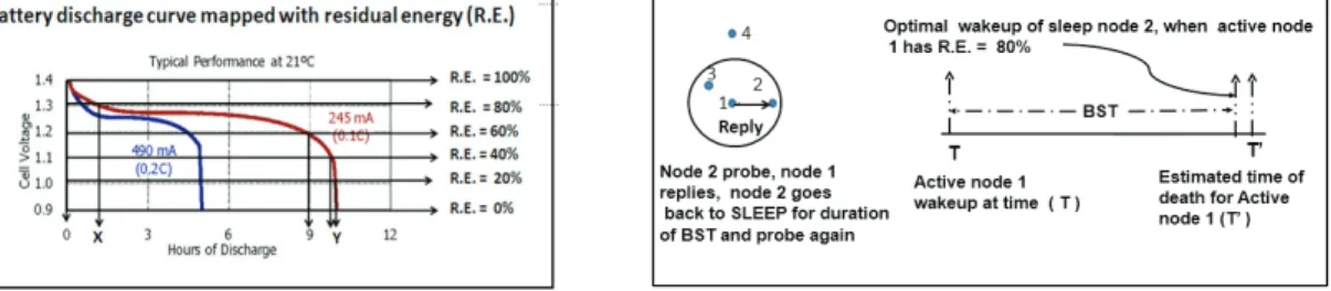
We proposeDCBSPprotocol for determining duty cycle of sensor nodes. In DCBSP the determination of duty cycle for sleeping nodes is based on optimalBackoffSleep Timederived from battery discharge curve. Fig.116shows
Fig. 1: Battery discharge curve16 Fig. 2: Optimal wakeup of DCBSP
discharge curve to determine the duty cycle for the neighboring sleeping nodes based on residual energy of an active node. For example, if residual energy of a current active node is 80%, which indicates that current active node has consumed 20% of its total energy. From figure 1, we observe that the time required for 20% of energy consumption is approximately ’X’=1.5 hrs we call this time asCurrent Consumption Time. Similarly, the time requires for active node to consume 100% of energy is approximately ’Y’=10 hrs from figure 1 we call this time asTotal Discharge Time. TheTotal Discharge Timeindicates that, after 10 hrs of operation, battery will be fully discharged. Hence, we derive theBackoffSleep Timeas
BackoffSleep Time=Total Discharge Time−Current Consumption Time (1)
The wake-up cycle for a sleeping node in DCBSP is explained with the help of an example. Figure 2 shows four deployed nodes where node 1 is active state and reaming nodes (2,3,4) are in the sleep state. The sleeping nodes (2,3) are within sensing range of active node 1. Node 1 has a residual energy of 80%. This means that its battery would discharge fully after approximately 8.5 hrs from figure 1 and equation 1. Node 2 is in the sensing range of node 1. Hence, node 1 replies to the probe of node 2. This reply contains theBackoffsleep time(BST)=8.5 hrs. Hence, node 2 goes into sleep state for the time duration ofBST. Thus, in DCBSP the sleeping nodes wake-up close to the death of the active nodes which ensures that energy is not wasted in unnecessary wake-ups. In the next subsection, we describe the probing mechanism with the help of state and flow transition diagrams of DCBSP.
3.2. State Transition and flow diagram of DCBSP
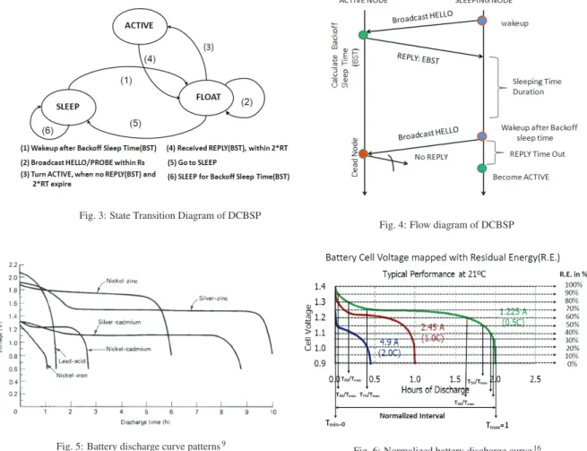
Each node in DCBSP has three operating states which are similar to RBSP8:SLEEP,FLOAT andACTIVE. The
state transition diagram for all three modes is shown in figure 3. In the SLEEP state, a node turns its radio offto conserve energy. Each node in FLOATING state broadcasts HELLO message within its sensing rangeRs, whereRs
is the maximum sensing range within which an event can be observed or detected. The ACTIVE node continuously senses the physical environment and communicates with other sensor nodes. The flow diagram of DCBSP is shown in fig. 4. Nodes are initially in sleeping state where each node sleeps for a backoffsleep time interval which is a small random time. After the node wakes up, it enters into a FLOATING state. The FLOATING node broadcasts HELLO message within its sensing rangeRs. If active node/nodes within the sensing range responds with a REPLY message which includes aBackoffSleep Time(BST), then its state changes to SLEEP mode. The FLOATING node waits for
Reply Time Out(RTO)which is the time interval between sending HELLO packet to receipt of REPLY message. The floating node estimated the RTO as 2∗ Rs
c, where c is the velocity of light. If the FLOATING node does not hear any REPLY in any RTO period, it enters into ACTIVE state and starts its timer to measure the current working time
Tcurrent. The current working timeTcurrentis define as the time elapsed from the instant the floating node turns active. In DCBSP, if floating node enters into the ACTIVE state, the node remains active until it consumes all of its energy. Thus, by using DCBSP each sleeping node determines itsACTIVEandSLEEPcycle based on the residual energy of current active node. In the next subsection, we describe how DCBSP computes BST at an active node, using battery discharge curve.
Fig. 3: State Transition Diagram of DCBSP
Fig. 4: Flow diagram of DCBSP
Fig. 5: Battery discharge curve patterns9
Fig. 6: Normalized battery discharge curve16
3.3. Estimation of BackoffSleep Time (BST)in DCBSP)
The battery discharge curve can accurately represent the behavior of many battery types as shown in figure 59,
provided the parameters are well determined. According to reference9, all the batteries including Zinc, Nickel-Cadmium, Silver-Nickel-Cadmium, Silver-Zinc and Lead Acid batteries follow the same pattern of discharge, even when current rating or load conditions are different. In figure 616there are three discharge curves, each having different
current rating such as 4.9A, 2.45A and 1.225A. In our protocol design, we have used the discharge curve for a constant current of 1.225A (0.5 C rate1), which indicates that after 2 hours of operation, battery will be fully discharged. This selection of battery discharge curve does not have an impact on our results, since the curve follows the same pattern of discharge even in case of different current rating. Similarly, for a constant current of 2.45A (1.0 C rate1), the battery will be fully discharged after 1 hour. This indicates that, the discharge time of a battery is dependent on the current rating or load conditions. However, to simplify the computation we create a battery discharge curve with a normalized time range of 0 to 1 as shown in figure 6. Here,Tmin is the minimum time and is set to 0 while,
Tmaxis the maximum time and is set to 1. Normalized curveis a generic battery curve used for computations. The normalized discharge curve is used to estimate the fraction of time remaining for battery discharge. Once the fraction ofNormalized Current Time(NCT) for particular energy level has been determined from the normalized discharge curve thende-normalizationis done to obtained actual full discharge time of battery. This actual full discharge time of battery value is used to calculate BST.
In our protocol, each node has10residual energy levels. The residual energy levels are mapped by using the battery discharge curve9as shown in figure 6. To compute the normalized time values, we first divide curve into 10 equals
parts across the y-axis. We note the y-axis values for each of the intercepts of these 10 lines across the y axis. Let, each node initially start from residual energy leveli=10, where it’s residual energy is between 90%<R.E.≤100%. If an active node has 100% residual energy, theNormalized Current Time(NCT) for node isTT100max as shown in figure 6. When the active node consumes more than 10% of its residual energy, its residual energy level changes toi=9 where its residual energy is between 80%< R.E. ≤ 90%. Therefore, theNCT for 90% of residual energy is TT90max. In this
way, when the node consumes more power, residual energy level becomes low and theNCT approaches unity (Tmax =1). According to the above mechanism, theNormalized Current Time(TT100
max, T90 Tmax, T80 Tmax... T10
Tmax) based on residual
energy levels is computed. We usedinterpolation17to compute intermediate values of theN
CT.
The residual energy fraction (Normalized Current Time) is known from the normalized battery curve using inter-polation. The actual current timeTcurrenthas been measured by the active node. Using the normalized discharge curve andTcurrent, in effect, we create a battery discharge curve for the prevailing load. Using these two values the actual full discharge time of the battery can be determined, we call thisde-normalizationof theNormalized Current Time (NCT). This is done using equation 2.
TDischarge=
Tcurrent
Normalized Current Time(NCT) (2)
Where,Tcurrent is the current working time of active node. TDischarge is actual full discharge time or de-normalized time and it indicates that afterTDischargehours of operation, the battery will be fully discharged. Therefore, theBackoff
Sleep Time (BST)is calculated by the active node as follows:
BackoffSleep Time(BST)=TDischarge−Tcurrent (3)
In this way, theBackoffSleep Time (BST)is derived by the active node based on battery discharge curve. In the next section, we evaluate the performance of DCBSP and compare it with PECAS, RBSP and PEAS.
4. Simulation results
We have implemented DCBSP in ns-218. The energy model, in this protocol, is similar to RBSP8, where Sleep:Idle
:Tx:Rx as 0.03mW:12mW:60mW:12mW. We assume that, the maximum sensing range is 5 meters and is equal to the transmission range for initial setup. The initial energy of each node is set at 2 Joule. We run the simulation for 300 sec. The packet size of HELLO and REPLY messages are 25 bytes each. We deployed 100 sensor nodes over 50×50m2network field. Nodes are randomly deployed in the field and remain stationary after deployment. We ran
each simulation 5 times and represent the average result of the 5 runs.
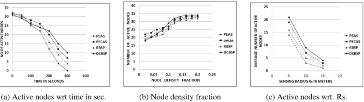
We have usedactive node countas one of the parameter for evaluating the performance of DCBSP. Theactive node countover time as a measure for the lifetime of coverage in the network. So, protocol with large number of active node for a longer duration is better for maintaining adequate coverage. We conduct simulations with varying node density and varying sensing range to evaluate the performance of DCBSP under varying conditions. We can see that even under varying conditions DCBSP gives better performance than PECAS, RBSP and PEAS. Figure 7(a) shows the total number of active nodes with respect to time. We can see that DCBSP has larger number of active nodes at the end of simulation at 300 seconds. DCBSP has 33%, 21% and 11% of active nodes as compared to PEAS, RBSP and PECAS respectively.
Thenode density fractionis an important parameter in wireless sensor networks. The node density fraction is the ratio of number of deployed nodes to the total area of the network field. Figure 7(b)shows the number of active nodes with varying node density. DCBSP and other protocols maintain adequate active nodes in order to monitor the intended network field. As compared to other protocols theactive node countin DCBSP increases with respect to node density. This shows that, DCBSP performance improves as the node density increases. DCBSP is able to scale and perform better even at higher node density.
DCBSP considers uniform circular sensing range. An event that occurs within the sensing range of node is assumed to be detected with probability of1while any event outside the range is assumed to be of0. Sensing range of a node in sensor network, effects the count of active nodes. As sensing range of node increases, the sensing area per node is also increases in proportion. Hence, the total number of nodes are required to monitor the entire network field will be less in such case. We varied the sensing range as 5, 10, 15 meters. Figure 7(c) shows the average number of active
(a) Active nodes wrt time in sec. (b) Node density fraction (c) Active nodes wrt. Rs.
Fig. 7: Performance of number of active nodes wrt time and Rs, node density fraction
(a) Average energy consumption (b) Coverage ratio wrt. time (c) Average coverage ratio wrt. Rs
Fig. 8: Performance of average energy consumption and coverage ratio
nodes with respect to sensing range(Rs). The number of active nodes in DCBSP are more than that of other protocols due to optimal wake-ups of sleeping nodes.
Figure 8(a) shows the average energy consumption of network with respect to time. The average energy consump-tion is the ratio of total energy consumpconsump-tion to total number of nodes in the network. The average energy consumpconsump-tion of DCBSP is lesser than that of PEAS by 39% and lesser by 25% and 15% as compared to RBSP and PECAS respec-tively. Hence, DCBSP is effective for extending the network lifetime.
Any coverage protocol for sensor networks needs to achieve adequate coverage of sensing region. Therefore, we need to keep sufficient number of nodes in active state. Hence, our aim is to keep sufficient number of nodes in active state while ensuring adequate coverage with minimum energy consumption. Therefore, we have considered coverage ratio as performance parameter in our simulation. For our scenario, it is worth noting that ratio of the entire sensing area to the maximum sensing area per node is about 50π∗∗(5)502 ≈ 31, which implies that at least 31 nodes are required to cover the entire area. We definedcoverage ratioas the number of active nodes in the sensing field to the minimum number of active nodes required to monitor entire region of networks. So the coverage ratio is given by
Active−Nodes−Count
31 . We have plotted the graph of coverage ratio by determining the count of active nodes at
100-200-300 seconds. Here, we have ignored the coverage area overlap of the active nodes in the networks. From figure 8(b), DCBSP protocol provides approximately 38% of coverage ratio while PECAS, RBSP and PEAS provide 20%, 16% andzerocoverage at the instant of 300 seconds. Beside the coverage ratio, Figure 8(c), shows the effect of sensing range on the average coverage ratio. We can see that DCBSP is able to maintain higher coverage even at higher sensing range. The performance improvement due to DCBSP is maintained at higher sensing range also.
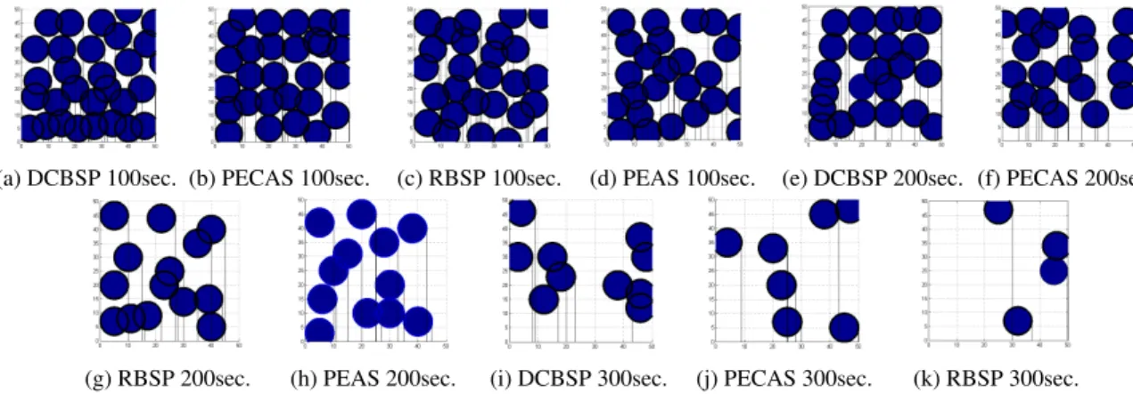
We also need to evaluate the actual area coverage based on the position of active nodes in the networks. We use the active node position to plot the node sensing region as dark circle and the image processing function in MATLAB to determine area coverage. This is shown in figure 9 (a to k). The circular shaded area indicates that node is active and monitors the field while white portion indicates no active nodes monitor the field i.e. region is uncovered. For example, in figure 9(i) the percentage of shaded area is 31.84% which indicate that, for DCBSP protocol, area coverage is 31.84% at the instant of 300 seconds. Similarly, the area coverage is 25.90%, 14.88%, zero coverage for PECAS, RBSP and PEAS for the same instant. The values for 100, 200 and 300 seconds for DCBSP and other protocols are
(a) DCBSP 100sec. (b) PECAS 100sec. (c) RBSP 100sec. (d) PEAS 100sec. (e) DCBSP 200sec. (f) PECAS 200sec.
(g) RBSP 200sec. (h) PEAS 200sec. (i) DCBSP 300sec. (j) PECAS 300sec. (k) RBSP 300sec.
Fig. 9: Area coverage at 100 seconds, 200 seconds and 300 seconds of DCBSP, PECAS, RBSP and PEAS
given in table 1 based on figure 9(a-to-k). From the above results, we can observe that DCBSP protocol gives better results as compared to PECAS, RBSP and PEAS due to its optimal wakeup cycle.
Table 1: Percentage of coverage area based on figure 9 Protocols DCBSP PECAS RBSP PEAS 100 seconds 82.87% 83.56% 75.74% 71.91% 200 seconds 73.45% 63.15% 47.17% 42.62% 300 seconds 31.84% 25.90% 14.88% 00%
5. Conclusions and future work
We have proposed a Discharge Curve BackoffSleep Protocol(DCBSP) which is a location unaware protocol that depends on BackoffSleep Time derived from the battery discharge curve. Based on optimalBackoffSleep Time, DCBSP avoids random and unnecessary frequent wake-ups of sleeping nodes. Due to this, sleeping nodes wake-up only at the required instant of time. This leads to less energy consumption and increased network lifetime. DCBSP allows the redundant sensor nodes to enter intosleepstate while it is possible to keep sufficient count of nodes in
active state in order to monitor the required network field.
The simulation result shows that DCBSP has sufficient count of active nodes in order to maintain adequate sensing coverage ratio. The area coverage ratio of DCBSP is 73.45% for the instant of 200 second while 63.14%, 47.17% and 42.62% for PECAS, RBSP and PEAS. The average energy consumption of DCBSP is lesser than that of PEAS by 39% and less by 25% and 15% as compared to RBSP and PECAS respectively. DCBSP maintains higher, longer coverage ratio and network lifetime as compared to other protocols. In future work, we plan to extend our protocol for providing K-coverage, in order to obtain 100% coverage ratio in an energy efficient manner. Further, we plan to extend DCBSP to handle varying sensing node ranges and other network challenges.
References
1. V. Raghavendra, R. Kulkarni, F. A., K. Ganesh Venayagamoorthy, Computational intelligence in wireless sensor network: A survey, IEEE Communication Surveys and Tutorials 13 (1) (2011) 68–96.
2. K. Akkaya, M. Younis, A survey on routing protocols for wireless sensor networks, Science Direct, Ad Hoc Networks 3 (2005) 325–349. 3. R. Mulligan, M. Ammari, Coverage in wireless sensor networks: A survey, Network Protocols and Algorithms 2 (2) (2010) 27–53. 4. I. Akyildiz, W. Su, Y. Sankarasubramaniam, E. Cayirici, Wireless sensor networks: A survey, Elsevier, Computer Networks 38 (4) (2002)
393–422.
5. A. Ghosh, S. Das, Coverage and connectivity issues in wireless sensor networks: A survey, Science Direct, Pervasive and Mobile Computing 4 (2008) 303–334.
6. F. Fan Ye, G. Zhong, J. Cheng, S. Lu, L. Zhang, Peas: A robust energy conserving protocol for long-lived sensor networks, 23rd International Conference on Distributed Computing Systems(DCS’ 02) (2002) 28–37.
7. C. Gui, P. Mohapatra, Power conservation and quality of surveillance in traget tracking sensor networks, in: Proceedings of 10th Annual International Conference on Mobile Computing and Networking (ACM MobiCom’ 04), Pennsylvania, USA, 2004, pp. 129–143.
8. A. More, V. Raisinghani, Random backoffsleep protocol for energy efficient coverage in wireless sensor networks., Smart Innovation, System and Technology, Springer, Varlag 28 (2) (2014) 323–331.
9. M. Crompton., Battery Reference Book, Reed eductaional and professional publishing ltd, Linacre House, Jordan Hill, Oxford OX2 8DP 225 Wildwood Avenue, Woburn, MA 01801-2041, 2000.
10. G. Xing, X. Wang, Y. Zhang, C. Lu, R. Pless, C. Gill, Integrated coverage and connectvity configuration for energy conservation in sensor networks, ACM Transactions on Sensor Networks 1 (1) (2005) 36–72.
11. S. Zhang, Y. Yuhen Liu, J. Pu, X. Zeng, Z. Xiong, An enhanced coverage control protocol for wireless sensor networks, 42nd Hawaii International Conference on System Sciences, HICSS’ 09 (2009) 1–7.
12. H. Zhang, J. Hou, Maintaining sensing coverage and connectivity in large sensor networks, Ad Hoc and Sensor Wireless Networks 1 (2005) 14–28.
13. M. Hefedda, H. Ahmadi, Energy-efficient protocol for deterministic and probabilistic coverage in sensor networks, IEEE Transactions on Parallel and Distributed Systems 21 (05) (2010) 579–593.
14. S. Jayashree, B. Manoj, S. Murthy, On using battery state for medium access control in ad hoc wireless networks, MobiCom04, Philadelphia, Pennsylvania, USA.
15. C. Chiwoo, P. Jinsuk, K. Jinnyun, L. Icksoo, H. Kijun, A random backoffalgorithm for wireless sensor networks., Next Generation Teletraffic and wired/wireless Advanced Networking, LNCS, Springer 4003 (5) (2006) 108–117.
16. EBC-7102I data sheet - energizer holdings inc.
17. L. Scott, Numerical Analysis, Princeton university press, 41 William Street, Princeton, New Jersey, USA, 08540-5237, 2011. 18. ns-2, Network Simulator,http://www.www.isi.edu/nsnam/ns, [Online; accessed 24-Dec-2014] (2013).