NBER WORKING PAPER SERIES
FEDERAL BUDGET RULES:
THE US EXPERIENCE
Alan J. Auerbach
Working Paper 14288
http://www.nber.org/papers/w14288
NATIONAL BUREAU OF ECONOMIC RESEARCH
1050 Massachusetts Avenue
Cambridge, MA 02138
August 2008
This paper was presented at a conference on Fiscal Rules and Institutions organized by the Economic
Council of Sweden, Stockholm, October 2007. I am grateful to my discussant, Torbjörn Becker, to
other conference participants, and to Dhammika Dharmapala, Bill Gale, Richard Kogan and Dan Shaviro
for comments on earlier drafts. The views expressed herein are those of the author(s) and do not necessarily
reflect the views of the National Bureau of Economic Research.
NBER working papers are circulated for discussion and comment purposes. They have not been
peer-reviewed or been subject to the review by the NBER Board of Directors that accompanies official
NBER publications.
© 2008 by Alan J. Auerbach. All rights reserved. Short sections of text, not to exceed two paragraphs,
may be quoted without explicit permission provided that full credit, including © notice, is given to
the source.
Federal Budget Rules: The US Experience
Alan J. Auerbach
NBER Working Paper No. 14288
August 2008
JEL No. D78,H62,J11
ABSTRACT
Like many other developed economies, the United States has imposed fiscal rules in attempting to
impose a degree of fiscal discipline on the political process of budget determination. The federal government
has operated under a series of budget control regimes that have been complex in nature and of debatable
impact. Much of the complexity of these federal budget regimes relates to the structure of the U.S.
federal government. The controversy over the impact of different regimes relates to the fact that the
rules have no constitutional standing, leading to the question of whether they do more than clarify
a government's intended policies.
In this paper, I review US federal budget rules and present some evidence on their possible effects.
From an analysis of how components of the federal budget behaved under the different budget regimes,
it appears that the rules did have some effects, rather than simply being statements of policy intentions.
The rules may also have had some success at deficit control, although such conclusions are highly
tentative given the many other factors at work during the different periods. Even less certain is the
extent to which the various rules achieved whatever objectives underlay their introduction.
Alan J. Auerbach
Department of Economics
508-1 Evans Hall, #3880
University of California, Berkeley
Berkeley, CA 94720-3880
and NBER
Like many other developed economies, the United States has imposed fiscal rules in attempting to impose a degree of fiscal discipline on the political process of budget
determination. But the U.S. experience has differed from that of the European Union under the Stability and Growth Pact, for example, in that U.S. budget rules operate at different levels of government. Relatively tight rules apply at the level of U.S. states, with virtually all states operating under some sort of annual balanced budget requirement, with the consequence that state fiscal responses to budget shocks tend to be rapid and sharp.1 At the national level, however, occasional attempts over the years to pass a balanced-budget amendment to the U.S. constitution have not succeeded, and the federal government has operated under a series of budget control regimes that have been complex in nature and of debatable impact.
Much of the complexity of these federal budget regimes relates to the structure of the U.S. federal government, with its constitutionally specified separation of powers between the legislative and executive branches and its bicameral legislature, which often has different operating rules and procedures in the House and the Senate. The controversy over the impact of different regimes relates to their temporal nature: as the rules are adopted by the
government to which they apply and have no constitutional standing, they can be (and have been) frequently modified over time, leading to the question of whether the rules do more than clarify a government’s intended policies.
In this paper, I review the federal budget rules that have been practiced in the United States in recent decades and present some evidence on the effects that these rules may have had on the fiscal policies of the federal government. Although the focus is primarily positive in nature – what the rules have accomplished – I will also touch on the normative question of how rules might be designed.
1
1. Budget Regimes
The modern period for U.S. budget policy is often viewed as dating from 1974, with the passage of the Congressional Budget Act (CBA). The CBA elevated the role of Congress in the budget process, establishing a Budget Committee in each house of Congress and creating the Congressional Budget Office (CBO) to provide budget projections needed to implement the legislation. Under the CBA, both houses of Congress pass a resolution laying out limits on revenues and spending for the coming year, and subsequent legislation is supposed to adhere to these limits.
The CBA provided a coordination mechanism for Congressional budget actions, and also introduced the practice of providing multi-year budget projections to Congress, a practice that eventually would play a role in the formulation of budget rules. However, the CBA did not restrict the size of government or the ability of government to increase spending or cut taxes. Indeed, historically large (as a share of GDP) peacetime deficits followed soon after, in the 1980s, as a consequence of the very large Reagan tax cuts in 1981 and two recessions, one very severe, early in the decade.2
In late 1985, Congress passed the Gramm-Rudman-Hollings (GRH) bill, which specified a series of annual deficits to be achieved, culminating in a balanced budget in fiscal year 1991. The legislation required that the budget the President submitted each year be consistent with that year’s deficit target, and that Congress pass legislation in accord with the deficit target. If legislated policy was projected to miss the deficit target, then an automatic “sequestration” process would ensue, cutting the budget according to a specified allocation rule in order to meet the deficit target. The sequestration procedures were modified in 1987 after the first version of GRH was found unconstitutional by the Supreme Court on the basis
2 Although there was also a large increase in defense spending during the period, there was also a cut in
non-defense spending, so that there was little overall trend in federal spending as a share of GDP during this period. See Figure 1 below and, for further discussion, Auerbach (2006a).
that Congress had assumed a role constitutionally reserved for the Executive branch; the 1987 legislation also relaxed the target deficit reduction path to one in which a zero deficit was to be achieved in 1993, rather than in 1991.
The sequestration process was avoided while GRH remained in force, but the
combination of declining target deficits and a recession that began in the summer of 1990 led to a budget crisis when policies producing very large deficit cuts would have been required to stay on the prescribed deficit path. In the fall of that year, as the culmination of a protracted “budget summit” meeting of President George H. W. Bush and leaders of Congress, GRH was scrapped and replaced with the Budget Enforcement Act (BEA).
The BEA eliminated annual deficit targets and instituted targets for discretionary spending, a category that excludes social insurance spending for health, Social Security (public retirement and disability pensions), unemployment and other “entitlement” programs. For the budget as a whole, BEA specified “pay-as-you-go” (PAYGO) restrictions on taxes and entitlement spending (other than Social Security), requiring that legislation on such items not increase the deficit, in the aggregate. Thus, except for discretionary spending, the budget rule now applied to legislated changes in policy, rather than to actual levels of spending or revenue. Changes in taxes or entitlement spending that resulted from economic growth, inflation, shifts in the income distribution or any other economic factors not directly
attributable to policy actions were ignored when determining if the budget rule were satisfied. Thus, any cyclical or trend movements in the deficit, revenues or expenditures, except those associated with discretionary spending, were left outside the process.
The BEA also introduced the use of a multi-year budget “window,” requiring initially that the PAYGO requirement be satisfied over a five-year period, based on CBO projections, rather than just for the immediate fiscal year in which legislation was enacted. The aim of including several years was to incorporate the future effects of policy actions and to reduce
the scope for using short-term timing changes to meet a one-year deficit target. The BEA originally applied through 1995, but it was extended to 1998 and then to 2002 by legislation in 1993 and 1997, respectively, before officially expiring in 2002.
For much of the period during which the BEA was in force with respect to Congressional legislation, the Senate followed additional rules with respect to its own operations.3 In 1993, the Senate adopted a 10-year PAYGO rule. In addition to imposing a longer horizon on budget policy, the Senate rule also effectively included a supermajority provision: a point of order could be raised in objection to legislation that violated the PAYGO rule, and 60 votes (of 100 in the Senate) are required to overrule a valid point of order.
Another restriction on Senate budget policy was included in the so-called Byrd rule (adopted in 1983), which made subject to a point of order certain proposals that would
increase the deficit beyond the budget window. The Byrd rule became quite relevant in 2001, when the tax cuts proposed by President George W. Bush were adopted for only a ten-year period. Because of the possibility that Republicans would be unable to muster 60 votes to override the point of order based on the Byrd rule, the tax cuts were enacted to apply only during the budget window. Although there have been subsequent modifications to some provisions of the 2001 legislation, current law still specifies that marginal income tax rates will rise in 2011 to their pre-2001 levels, and that the federal estate tax, having been fully phased out in 2010, will reappear in 2011 in its pre-2001 form.
Although the BEA was officially in place through 2002, it began to erode after 1998, the fiscal year in which the United States had its first budget surplus since the 1960s. At first, the erosion took the form of procedures used to get around the BEA’s restrictions. For example, 1999 saw a huge increase in “emergency” discretionary spending, a spending category not subject to the BEA’s discretionary spending caps (CBO 1999); much of this
3
spending had little to do with actual emergencies. Eventually, however, Congress simply changed the budget rules as it went, adjusting the discretionary spending caps to conform to actual spending and setting aside the PAYGO rules on a case-by-case basis, even before they expired. Thus, it was possible to adopt a large tax cut in 2001 with no offsetting revenue increases or entitlement spending reductions, even though BEA was still officially in force.
In the years since, Congress has acted essentially without budget rules of the type embodied in GRH or BEA, even though it has used the Congressional Budget Act and the annual budget plans it requires to impose limits on the budget effects of certain legislation, as in 2003, when a 10-year budget cost of $350 billion was imposed before the details of a tax cut were worked out. (This episode is discussed further below.) The 2007 change in the control of Congress that resulted from the November, 2006 elections has led to a renewal of interest in budget rules and the enactment by the House and Senate of 10-year PAYGO rules applicable to the consideration of legislation by these bodies, although this development comes after the sample period covered by the data analyzed below.
The repeal of GRH in 1990 and the collapse of BEA after 1998 both illustrate a characteristic of U.S. federal budget rules: the rules cease to operate once they deviate too far from consensus policy. In 1990, GRH called for deficit reduction far greater than Congress wished to enact. After 1998, adherence to BEA would have resulted in significant budget discipline for which Congress had little taste, given that the federal budget had moved into surplus and that CBO was projecting even larger surpluses for the years to come, assuming continued compliance with BEA’s discretionary spending caps and PAYGO rules.
That these rules should ultimately have failed is not surprising, given that they were adopted by majority vote and could be repealed by majority vote. Indeed, one might question whether they had any impact at all, given that they could be adjusted at will and indeed were frequently modified. That is, unlike a constitutional amendment which, once adopted, is very
difficult to repeal, U.S. federal budget rules have the same permanence as any other piece of legislation.
At the same time, it is possible that a change in the budget process, even if adopted by simple majority, can change budget outcomes, by altering each legislator’s incentives and ability to promote deficit-increasing legislation even while a majority continues to support the budget rule. For example4, suppose that each legislator prefers a low overall deficit to a higher one, but also wishes to promote his own spending priorities. Under this assumption, each legislator might prefer an equilibrium outcome of low spending and a low deficit to one with proportionally higher spending on all programs and a higher deficit. With no budget rule in place, however, there may be no commitment mechanism in place to facilitate cooperation on keeping spending low. Legislators may find it optimal to push their own spending
programs, knowing that other legislators will do the same; if any legislator failed to push his own program in this case, the deficit would still be high and he would lose out on the spending side. With an overall spending limit in place, however, the lobbying of individual members may cancel out, given that increasing spending for one program requires decreasing it for another. This could lead to an equilibrium outcome with proportionately lower spending and a low deficit, an outcome that legislators would prefer to the high-deficit-high-spending outcome with no budget rule. Thus, the outcome achieved under a budget rule might be consistent with the contemporaneous wishes of the majority, while at the same time representing a different outcome than would occur without the budget rule in place.
Even if budget rules shift the equilibrium with respect to the deficit and the level and composition of spending, there is a question of the extent to which the measured changes reflect real economic changes, as opposed to short-run timing or manipulations of accounting
4
rules. For instance, Reischauer (1990) estimates that half of the deficit reduction achieved during the GRH period fell into the “one-time savings” category including asset sales.
But there are more subtle types of timing and accounting manipulations than those that can be easily identified. In 1997, for example, Congress introduced a tax-favored saving scheme (the Roth Individual Retirement Account, or Roth IRA) that exempted returns from taxation, as an alternative to an existing scheme (the traditional IRA) that provided a tax deduction for contributions but then taxed all withdrawals of interest and principal. The legislation also offered tax incentives to switch funds from traditional IRAs to Roth IRAs. While the two schemes are economically similar (and equivalent when tax rates are constant over time), the timing of tax revenues differs between the two. The Roth IRA generates revenue losses of comparable present value as the traditional IRA, but these revenue losses occur later. Switches of funds from traditional IRAs into Roth IRAs actually increase short-run revenue by speeding up the payment of taxes on withdrawals from the traditional IRAs. Thus, the introduction of the Roth IRA was actually estimated to increase tax revenue over the budget window, even while representing a permanent reduction in the present value of tax revenue, because of the tax incentives provided for switching.5
As the preceding example illustrates, it difficult if not impossible to specify which budget changes are “real” and which are not, and this makes the task of measuring the effects of budget rules more difficult. So, too, does the absence of a counterfactual policy path, for determining whether policies followed under any particular budget rule would have occurred under a different budget regime.
With these obstacles in mind, it is helpful to consider many different types of evidence in trying to understand the potential impact of U.S. budget rules. Based on the discussion
5 The present value of tax revenue was also reduced by the fact that the overall limits to contributions to these
accounts are based on before-tax dollars, making the out-of-pocket contributions and hence the associated revenue loss smaller under the traditional IRA than under the Roth IRA.
above, one can distinguish up to five potentially distinct periods, depending on data
availability: (1) the era prior to the 1974 Congressional Budget Act, under which no explicit budget rules were in effect; (2) the CBA period, from the 1974 adoption of the CBA until the 1985 passage of the first Gramm-Rudman-Hollings Act, during which budget policy was coordinated but no exogenous restrictions on spending or taxes were imposed; (3) the GRH period, from late 1985 until the late-1990 adoption of the Budget Enforcement Act, during which explicit one-year deficit targets were specified; (4) the BEA period, from adoption of BEA until its effective demise around 1999, during which discretionary spending caps and PAYGO rules for taxes and entitlement spending were in force; and (5) the post-BEA period from 1999 to the present, during which limited budget rules have applied. To the extent that the rules of these different regimes were effective, one would expect the effects to be
different. We look for these differences in the analysis that follows
2. The Impact of Budget Rules
To provide a sense of how the U.S. budget evolved during the different policy regimes just described, I begin with some figures showing spending, revenues and the budget deficit over the past forty-five fiscal years.6
2.1. Overall Trends
Figure 1 shows total revenue and total non-interest spending at the federal level as a share of potential GDP, along with a breakdown of non-interest spending into three
components, entitlement spending, defense spending, and other discretionary spending. It is useful to break spending into these three components. Entitlement spending is less subject to year-to-year policy changes and also has a strong positive trend related to demographic shifts
6 All annual data are taken from the Congressional Budget Office web site, which when this paper was written
provided information for fiscal years 1962-2006. The U.S. fiscal year runs from October 1 of the previous calendar year through September 30 of the current calendar year.
and medical costs. Defense spending, even with the recent increase, has followed a
downward trend, with large temporary upward movements during the Vietnam War and the first part of the Reagan administration that were clearly not related to short-term budget conditions. Non-defense discretionary spending, on the other hand, shows no obvious trend as a share of potential GDP for the period as a whole, although there are minor trends during some of the budget regime sub-periods, including declines during the GRH and BEA periods and an increase in the most recent, post-BEA, period.
Total non-interest spending and revenue each average just over 18 percent of potential GDP for the period, again with no obvious trend for the period as a whole but sub-period trends, notably with spending falling and revenue rising during the BEA period and the reverse occurring in the post-BEA period.
Figure 2 presents the federal deficit as a share of potential GDP over the same period, simply the difference between total spending and revenues from Figure 1, plus debt service. The biggest trends here are the rise during the BEA period and the subsequent fall. The trends during these periods are reduced if one considers the full-employment surplus, and it is clear that the break in trend occurs not with the effective end of the BEA, dated here as after 1998, but with the transition from the Clinton administration to the Bush administrations. This distinction serves as a reminder that there were many changes in the policy environment occurring over the period, making it difficult to determine the particular impact of budget rules. It is therefore useful to focus on more subtle differences in revenue and spending patterns among the regimes, rather than simple trends in spending, revenue, and the budget deficit, which would be expected to vary with other important factors, such as the parties in control of the Presidency and Congress.
2.2. The Responsiveness of Discretionary Spending
As just discussed, non-defense discretionary spending experienced no overall trend as a share of potential GDP in the years since 1962. This spending category is perhaps the most susceptible to budget restrictions, given that entitlement spending is not directly driven by annual appropriations, and defense spending depends very strongly on factors external to the budget process. Moreover, discretionary spending has figured differently in the various budget regimes that have applied over time.
Absent any explicit budget rules, we might expect discretionary spending to increase with the health of the budget, as measured by the most recent budget surplus, if the surplus provides a signal of the resources available to the government. We might also expect
discretionary spending to increase with the size of the output gap between potential and actual GDP, based on Keynesian objectives to stimulate the economy when in recession or a period of slow economic growth.7
Table 1 provides estimates, based on annual fiscal year data, of the impact of the prior year’s budget surplus and output gap on the change in non-defense discretionary spending from the previous year, with all series scaled by potential GDP. The first column of the table presents this relationship estimated for the full sample period. As the column shows, this expected relationship holds weakly for the full sample period. The relationship is much stronger for the period prior to the Congressional Budget Act, as illustrated in the next column of Table 1. For the years 1963-1974, changes in non-defense discretionary spending rose by 17 cents for every dollar increase in the previous fiscal year’s budget surplus, and by 7 cents for each additional dollar by which actual GDP fell short of potential GDP. This represents
7
Such spending increases would largely reflect explicit policy actions, rather than automatic stabilizers, as most automatic stabilizers in the United States operate on the tax side, with revenues rising and falling with the level of economic activity. Those components of spending that do respond to the business cycle, such as
considerable sensitivity for a spending category that has averaged just below 4 percent of GDP over years.
This strong relationship entirely disappears during the CBA period, which overlapped the administrations of three presidents (from both parties), three recessions, and a rise and then a fall in non-defense discretionary spending. There were certainly large year-to-year changes in spending, but they appear not to have been related to the condition of the budget or the economy. Whether this change in responsiveness is attributable to the increased
coordination of spending facilitated by the CBA is difficult to assess. It may be that the change in responsiveness is related to the weakening of the power of Congressional committee chairs that happened around the same time, as a consequence of procedural reforms adopted during the post-Watergate era. These reforms may also have contributed to the jump in non-defense discretionary spending and entitlements at the beginning of the CBA period.
During the very short GRH period8, the very strong relationship of spending to the budget surplus reappears, but the response to the GDP gap does not. Although so short a sample period makes any conclusions tentative, both of these results are quite consistent with what one would expect, given the way that the GRH rules worked. As each year’s budget surplus was required to hit a pre-specified target, any improvement in the condition of the budget made more resources available for spending increases or tax cuts. But an increase in the output gap had no such effect, because the deficit targets were not adjusted for the business cycle.
8
I exclude from the sample the fiscal year during which GRH was adopted, 1986, because the adoption of GRH was accompanied by a very large cut in spending. Given the contemporaneous nature of these changes, it is hard to argue that the spending cut is attributable to the budget rule. I follow the same procedure below, excluding the observation that included the fiscal-year 1991 adoption of BEA, which resulted from a budget summit at which spending cuts and tax increases (which reversed President Bush’s campaign pledge of “no new taxes”) were also agreed to.
The behavior of discretionary spending under BEA was similar to that under CBA, not responsive to the budget surplus and not significantly responsive to the GDP gap. With discretionary spending caps in place, spending could only respond to the economy or to the budget if the caps themselves could respond, or if exceptions (such as emergency spending) could be arranged. The estimates suggest that neither of these channels was significant during the period, even though the caps were revised in 1993 and 1997 when the provisions of BEA were extended to later years. It must be noted that the majority of this period was one in which the President and Congress were controlled by different parties, with President Bush and a Democratic Congress during most of fiscal year 1992 and President Clinton and a Republican Congress during most of fiscal years 1995-98. An alternative explanation of the lack of spending responsiveness might be “gridlock” between the President and Congress, but split government (a Republican President and a Democratic Congress) also characterized most of the GRH period, when spending is estimated to have responded strongly to the budget.
In the most recent period, after the effective demise of BEA, discretionary spending has reverted to a pattern of significant responses to both the budget surplus and the GDP gap. The response to the surplus is weaker than under GRH, but this makes sense, given that there is no explicit deficit target.
These results are consistent with budget rules having had some impact on non-defense discretionary spending, although this conclusion applies to the responses of spending to the economy and the budget, and not necessarily to the level of spending itself. Except perhaps for the lack of responsiveness during the CBA period, the patterns are consistent with the restrictions imposed during the different budget periods, and so represent a more subtle form of evidence than that based on levels or the composition of spending, which might more easily be explained by alternative hypotheses regarding policy decisions during the different periods.
In short, it is hard to argue that this evidence is consistent with the budget rules being simply endogenous reflections of the policies of each period.
2.3. The Responsiveness of Spending and Revenue Legislation
Some elements of budget rules have involved levels of the deficit or its components. For example, GRH had deficit targets and BEA had caps on discretionary spending. But BEA also placed limits on legislated changes in spending and revenues, under its PAYGO rules. Thus, we should observe changes in patterns of these legislated changes if BEA had an impact.
To construct measures of legislated changes in revenue and expenditure, I utilize data and procedures developed in earlier papers, including Auerbach (2003, 2006). CBO typically publishes two major revisions in its projections of revenue and spending each year, in late January or early February, and in August or September. Each revision indicates the changes from the previous forecast and divides these changes into components due to legislation and to other factors. By accumulating changes attributed to legislative action between each of these forecasts (including intermediate revisions), one may derive a continuous, roughly semiannual series of forecast policy changes in revenue and spending, beginning with changes between winter and summer, 1984.9
For each observation, I measure the policy change with respect to revenue and non-interest spending. As each update includes legislative changes for the current fiscal year and several subsequent years, these must be combined in some manner to provide a measure of the legislation’s overall effect. I form the discounted sum of changes adopted during the interval for the current and subsequent four fiscal years (relative to each year’s corresponding measure
9
of potential GDP), with the five weights normalized to sum to 1 and a discount factor of 0.5.10 Just as current policy changes have effects in future fiscal years, policy may respond to future fiscal conditions as well. Thus, as an alternative to the most recent budget surplus, one might wish to use a measure based on the budget surpluses projected over the budget period, which are included in the CBO projections. To be consistent with the aggregate policy measure just developed, I aggregate the projected surplus for the current and next four fiscal years, as of the beginning of the period of observation, using the same discount factor as is used in constructing the policy measure.
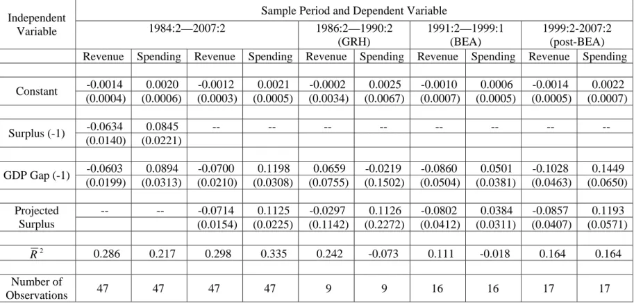
Table 2 presents results based on these constructed measures, starting with those for the full period available, beginning with the observation for change in projections from winter to summer 1984, labeled 1984:2, and ending with the changes in August, 2007. In the first two columns of the table, the explanatory variables are the previous fiscal year’s actual budget surplus, and the estimated GDP gap in the most recent quarter before the policy change being explained. For example, the gap from the last quarter of calendar-year 2006 is used for the last observation. The first column in Table 2 presents results for the full sample period with revenue as the dependent variable; the second column has the same specification but with non-interest spending as the dependent variable. Both sets of results show significant policy responses to both the budget surplus and the output gap, in the anticipated directions, with deficit-increasing policies resulting from higher surpluses or a higher output gap.
The third and fourth columns repeat these results, but with the weighted projected surplus included in place of the lagged surplus. While these two series are highly correlated, the projected surplus improves the fit of both regressions, and I will use this measure in the
10
That is, each successive future observation receives half the weight of the observation one period earlier. This discount factor was chosen in my earlier work based on analysis using a simple goodness-of-fit measure (the
regression’s adjusted R2). I reduce the weight on the current fiscal year by one-half and increase weights on
subsequent years correspondingly, for winter-to-summer revisions, as these revisions cover only part of the current budget year’s legislation.
remaining regressions. This change also increases the absolute value of all four coefficients of interest. For both specifications, the equations suggest that responses are somewhat larger on the spending side than on the revenue side, although these differences are not significant.
The lack of data from earlier periods means that we can consider the performance of these equations only for the three most recent budget regimes described above, GRH, BEA, and post-BEA. The results for each of these regimes, for both revenue and spending, are presented in the remaining columns in Table 2.11
For GRH, none of the coefficients are significant, but it is interesting to note that the coefficients on the GDP gap actually have the wrong sign, and do so only during this period.12 As discussed above in relation to a similar finding for discretionary spending, with binding deficit targets not adjusted for the level of economic activity, there is no scope for
countercyclical policy. Indeed, given that automatic stabilizers cause revenue to fall as output falls, the only way to keep the deficit from actually rising is to pass legislation to increase taxes or reduce spending as output falls – precisely the pro-cyclical legislative policy reactions estimated here.
Under the BEA regime, the regime for which these particular data on legislative changes are perhaps the most relevant, significant impacts for both output and surplus variables are restored on both the revenue side and the spending side. This result appears at first to be somewhat puzzling. After all, if the PAYGO rules are in place, then how can changes in the projected budget surplus or the output gap have any net impact on legislated changes in the deficit? A potential answer to this puzzle lies in the manner in which the PAYGO rules applied.
11
As before, I leave out the observations including the adoption of GRH (1986:1) and BEA (1991:1) to avoid attributing concurrent policy changes to the rules just being adopted.
12
The results for GRH are similar when the lagged budget surplus is substituted in the equation for the weighted projected surplus.
In simple terms, the PAYGO restrictions did not apply directly to the revenue and spending variables being measured here. First, the restrictions applied to legislation enacted in any given fiscal year, whereas the variables measured here are semiannual. Thus, the PAYGO rules could be satisfied by offsetting deviations in successive observations. Second, the PAYGO rules did not apply to the weighted sum of five years’ revenue or spending changes. Under the original PAYGO rule, deficit-increasing legislation was ruled out for each fiscal year prior to the end of the PAYGO period, 1995. This meant that legislation enacted in the first fiscal year of the period, 1991, faced restrictions over five fiscal years, legislation enacted in fiscal year 1992 faced restrictions over four fiscal years, and so on. When the PAYGO rules were extended in 1993, a new five-year horizon was established, ending in 1998, but this horizon again had a fixed date. Only with its final extension did the PAYGO rules apply to a five-year rolling horizon, but this happened only in 1997, nearly at the end of what I have classified as the effective PAYGO period.13 Thus, legislation was only partially restricted in the later years of the five-year budget window, so we might expect the overall response based on the five-year weighted average to be smaller than with no restrictions but not zero.
The Senate’s PAYGO rule, on the other hand, had a horizon even longer than the five years covered by the dependent variables in Table 2, but the restrictions did not apply to future years individually. Legislation could not increase the deficit in the current year or the first five years as a whole, but it could increase the deficit in any one of years 2-5. As the effects across years were simply added up with no discounting, it would be possible, for example, to use small tax increases (relative to GDP) in later years to offset larger tax cuts in earlier years (relative to GDP).
13
Thus, the nature of the PAYGO rules suggests that policy responses as measured in Table 2 might have been muted by the rules but not eliminated. The last two columns of the table are consistent with this conclusion, showing that all four policy responses strengthened after the demise of BEA.
In summary, the strength and signs of legislative policy responses under different budget regimes are consistent with how the budget rules in each regime worked: pro-cyclical policy responses under GRH, full policy responses after BEA, and muted policy responses under BEA.
That policy responses existed under BEA doesn’t mean that policy was particularly active. Figure 3 graphs the revenue and spending dependent variables used to measure policy changes for the regressions in Table 2. The solid lines in the figure represent the actual policy changes. It is clear from Figure 3 that the policy changes were generally of much smaller magnitude during the BEA period than during GRH or after BEA; the only change of large magnitude was the tax increase barely pushed through a reluctant Congress by President Clinton in the first months of his administration.
Figure 3 also shows, as dotted lines, the policy responses predicted by the full-sample models in Table 2. From a comparison of the predicted and actual policy responses, we can see two factors contributing to the more modest policy actions occurring under BEA. First, during the BEA period, there was much less volatility around the predicted values. There were many large changes in policy during GRH and the post-BEA period that are not picked up by the model. Thus, policy was less active during BEA, conditional on the policy
responses estimated in Table 2.
A second factor at work is that the predicted policy responses are of a smaller
magnitude during the BEA period, and not simply because of smaller estimated coefficients. That is, even using the predicted policy responses from a single model, based on the
full-sample coefficients, the predicted values are generally much smaller in average absolute value during the BEA period than before or after. In other words, one explanation for why policy wasn’t especially active during the BEA period, other than the gridlock that might have existed between the President and Congress, is that policy didn’t have to be active. There were no new recessions during this period, and the budget deficits were not as high as during the GRH period, nor were the surpluses as high as early in the post-BEA period. This may also help explain why BEA lasted as long as it did: the outcomes specified by the rules may simply have conformed relatively closely to the policies that would have been chosen without the budget rules in place.
Thus, BEA appears to have had some impact on the strength of policy responses, and may also have reduced the magnitude of policy changes arising from factors other than the state of the budget or the economy. BEA’s duration, as compared to GRH for example, may be due in part to the relative lack of stimuli for policy changes, although BEA also differed from GRH in important ways that may have made it more stable, notably in eliminating the inducement of pro-cyclical policy responses and in placing caps only on discretionary spending.14
2.4. Summary
As I have stressed, it is probably easier to uncover the impact of budget rules in the patterns of policy responses than in overall levels of spending or revenue, given that many other factors influence these aggregates. Nevertheless, it is still of interest what these aggregates looked like during the different regimes. Table 3 presents the average values of the dependent variables used in producing the estimates in Tables 1 and 2, for the full sample
14
It would be desirable to add political variables to Table 2, but this makes identification difficult. For example, the one Democratic administration during this sample period – the Clinton administration – overlaps
substantially with the BEA period. Adding a dummy variable for the Clinton administration, interacted with the other explanatory variables, leaves the coefficients for both the BEA period and Democratic administrations quite insignificant in both revenue and expenditure equations.
periods and for the different policy regime sub-periods. In addition to the actual means, the table also provides adjusted means – what the means in the different periods would have been under the estimated policy rules, but at the full-sample average values for the explanatory variables. Adjusting the means help to distinguish the impact of policy rules from differences underlying conditions.
The upper panel of Table 3 shows the average annual changes in non-defense
discretionary spending as a share of potential GDP, the dependent variable in Table 1. For the full sample, this series has an average close to zero, consistent with the absence of a strong trend for the series in Figure 1. The means are positive before CBA and after BEA and negative during the CBA period and especially during the GRH and BEA periods, consistent with budget rules having a downward impact on spending growth. But this intuitive pattern is upset when the means are adjusted, suggesting, for example, that the strong growth of
discretionary spending in recent years is a consequence of underlying economic conditions rather than the absence of budget discipline.
The lower panel of Table 3 shows the average semiannual legislative changes in revenue and non-interest spending as a share of potential GDP, the dependent variables in Table 2. The means indicate mild surplus reduction policy on both the revenue and spending side for the sample as a whole, with strong deficit reduction policy on both sides under GRH, a roughly deficit-neutral policy stance under BEA, and a very pro-deficit stance since then. While adjustment of the means does change the picture somewhat, this same categorization of the three regimes holds.
3. Further Lessons from the U.S. Experience
Even though the Budget Enforcement Act eventually became a victim of strong incentives for policy action, the post-BEA period does offer additional lessons concerning the effects of budget rule design. In particular, the long budget window used by the Senate during
its post-BEA deliberations appears to have had an impact on the pattern of tax legislation, making so-called “sunset” provisions more common in tax legislation.
Even though the PAYGO rule was no longer in force at the time, deliberations leading up to the 2003 tax cut included negotiations between the President and Congress, and between the two houses of Congress, over the size of the tax cut and its components. An agreement was reached by the leaders involved, all of the same party (Republican) to limit the tax cut to a total revenue cost of $350 billion over the ten-year budget window, with the revenue cost calculated as the simple sum of revenue losses over the ten years.
This calculation method meant that there was a trade-off under the cap between the annual cost of the tax cut and the number of years over which the tax cut applied: a temporary tax cut could have a larger annual cost. Also, with no discounting of future revenue costs, tax cuts that applied only during the early years of the ten-year period were larger relative to the size of the economy than those that applied only later in the ten-year period. This lack of discounting, along with the greater uncertainty that future tax cuts could be sustained, made temporary tax cuts that applied early in the budget window more attractive to tax-cut
proponents than tax cuts that were to be phased in only toward the end of the budget window. The outcome in 2003, not surprisingly, was a temporary tax cut expiring before the end of the budget window. (The actual tax cut expired roughly midway through the ten-year window, although a larger tax cut of shorter duration was also considered during the
deliberation process.) This experience illustrates that even weak budget rules or procedures can have some impact on the shape of legislation. It also provides a reminder that care is needed in the design of budget rules.15
15 Sunsets have also arisen in reaction to the Senate’s Byrd rule, discussed earlier in connection with the tax cuts
of 2001. When binding, the Byrd rule effectively forced tax-cut legislation to lapse at the end of the budget window.
A similar impact can be seen by looking at the GRH period, when only the immediate fiscal year was relevant to budget rules. Figure 4 shows the impact of legislation during three periods, CBA, GRH, and BEA, based on the semiannual data on legislation used to produce the results in Table 2.16 For each regime, I sum over all legislative changes the estimated amount of deficit reduction occurring in the year of enactment and in each of the four succeeding fiscal years, dividing the amounts for each piece of legislation by the level of potential GDP in the year enacted. One would normally expect permanent, deficit-reducing legislation, such as a tax increase, to produce an upward profile, given that the economy is growing over time. Indeed, this is the case under both CBA and BEA. In fact, deficit reductions during each of these periods were back-loaded, actually increasing deficits in the years of enactment, taking advantage of multi-year budget accounting to get some credit for the deficit reductions enacted for future years. Under GRH, by contrast, the deficit reduction pattern is weighted much more heavily toward the year of enactment, as the nature of
incentives under GRH would lead one to expect.
While the objective in 2003 was to limit the size of the tax cut, it was not to encourage temporary policies that front-loaded tax cuts. Likewise, the designers of GRH were interested in more than temporary deficit reduction. In each instance, a multi-year budget window with discounting of future revenue costs might have led to a more rational outcome; it would have provided some credit for future years’ deficit reduction under GRH, and would have reduced the cost of future tax cuts under the budget cap in 2003. But the ideal parameters of such adjustments would depend on a number of factors, such as the stability of government and the political costs of modifying existing policies.17
16
A similar figure, based on a shorter sample period and a slightly different methodology, may be found in Auerbach (1994). There are only three observations for the CBA period.
17
4. Conclusion
The United States has experimented with a variety of budget rules in recent decades, none of which had the permanence of constitutional restrictions and all of which eventually gave way. From an analysis of how components of the federal budget behaved under the different budget regimes, it appears that the rules did have some effects, rather than simply being statements of policy intentions. These effects are largely consistent with how the budget rules worked. In some instances, as with induced pro-cyclical policy under Gramm-Rudman-Hollings or the 2003 sunset provisions, there were some clear negative side-effects. The rules may also have had some success at deficit control, although such conclusions are highly tentative given the many other factors at work during the different periods.
Even less certain is the extent to which the various rules achieved whatever objectives underlay their introduction, objectives which have not been discussed in this paper but presumably relate to the growth of government and to the tendency to shift financial
responsibilities to future generations. Achievement of such objectives requires not only that the rules matter, but also that the impacts conform to these underlying objectives. None of the U.S. budget rules studied here, for example, incorporates the implicit liabilities associated with the long-term commitments of entitlement programs. As a consequence, it has been possible to engineer large increases in future implicit liabilities with only limited impact on short-term budget measures. As economies evolve, a narrow perspective with respect to liabilities and commitments is an increasingly serious shortcoming.
References
Auerbach, A. J. (1994), The U.S. fiscal problem: where we are, how we got here, and where we’re going, in S. Fischer and J. Rotemberg (eds.), NBER Macroeconomics Annual, MIT Press, Cambridge, MA.
Auerbach, A. J. (2003), Fiscal policy, past and present, Brookings Papers on Economic Activity, 2003, 75-138.
Auerbach, A. J. (2006a), American fiscal policy in the post-war era: an interpretive history, in R. Kopcke, G. Tootell, and R. Triest (eds.), The Macroeconomics of Fiscal Policy, MIT Press, Cambridge, MA.
Auerbach, A. J. (2006b), Budget windows, sunsets, and fiscal control, Journal of Public Economics 90, 87-100.
Bohn, H., and Inman, R. (1996), Constitutional limits and public deficits: evidence from the U.S. states, Carnegie-Rochester Conference Series on Public Policy 45, 13-76. Congressional Budget Office (1999), Emergency Spending Under the Budget Enforcement
Act: An Update, U.S. Government Printing Office, Washington.
Dharmapala, D. (2006), The Congressional budget process, aggregate spending, and statutory budget rules, Journal of Public Economics 90, 119-141.
Heniff, B., Jr. (2007), Budget enforcement procedures: Senate’s pay-as-you-go (PAYGO) rule, Congressional Research Service paper.
Poterba, J.M. (1997), Do budget rules work? in A. Auerbach (ed.), Fiscal Policy: Lessons from Economic Research, MIT Press, Cambridge, MA.
Reischauer, R.D. (1990), Taxes and spending under Gramm-Rudman-Hollings, National Tax Journal 43, 223-32.
Table 1. Determinants of Non-Defense Discretionary Spending Changes, 1963-2006
Dependent Variable: Annual Change in Spending Relative to Potential GDP
(standard errors in parentheses)
Sample Period Independent Variable 1963-2006 1963-1974 (Pre-CBA) 1975-1985 (CBA) 1987-1990 (GRH) 1992-1998 (BEA) 1999-2006 (post-BEA) 0.0011 0.0036 -0.0002 0.0052 -0.0012 0.0010 Constant (0.0005) (0.0007) (0.0033) (0.0008) (0.0014) (0.0003) 0.0525 0.1783 -0.0199 0.1605 -0.0042 0.0684 Budget Surplus (-1) (0.0215) (0.0398) (0.1431) (0.0232) (0.1228) (0.0275) 0.0278 0.0668 -0.0250 0.0203 0.0597 0.0748 GDP Gap (-1) (0.0171) (0.0165) (0.0829) (0.0256) (0.1773) (0.0340) 2 R 0.084 0.719 -0.229 0.953 0.155 0.377 Number of Observations 44 12 11 4 7 8
Table 2. Determinants of Policy Changes, 1984-2007
Dependent Variable: Semiannual Policy Change in Revenue or Spending (Excluding Interest) Relative to Potential GDP
(standard errors in parentheses)
Sample Period and Dependent Variable Independent Variable 1984:2—2007:2 1986:2—1990:2 (GRH) 1991:2—1999:1 (BEA) 1999:2-2007:2 (post-BEA) Revenue Spending Revenue Spending Revenue Spending Revenue Spending Revenue Spending
-0.0014 0.0020 -0.0012 0.0021 -0.0002 0.0025 -0.0010 0.0006 -0.0014 0.0022 Constant (0.0004) (0.0006) (0.0003) (0.0005) (0.0034) (0.0067) (0.0007) (0.0005) (0.0005) (0.0007) -0.0634 0.0845 -- -- -- -- -- -- -- -- Surplus (-1) (0.0140) (0.0221) -0.0603 0.0894 -0.0700 0.1198 0.0659 -0.0219 -0.0860 0.0501 -0.1028 0.1449 GDP Gap (-1) (0.0199) (0.0313) (0.0210) (0.0308) (0.0755) (0.1502) (0.0504) (0.0381) (0.0463) (0.0650) -- -- -0.0714 0.1125 -0.0297 0.1126 -0.0802 0.0384 -0.0857 0.1193 Projected Surplus (0.0154) (0.0225) (0.1142) (0.2272) (0.0412) (0.0311) (0.0407) (0.0571) 2 R 0.286 0.217 0.298 0.335 0.242 -0.073 0.111 -0.018 0.164 0.164 Number of Observations 47 47 47 47 9 9 16 16 17 17
Table 3. Average Policy Changes
Annual Change in Non-defense Discretionary Spending Relative to Potential GDP
Sample Period 1963-2006 1963-1974 (pre-CBA) 1975-1985 (CBA) 1987-1990 (GRH) 1992-1998 (BEA) 1999-2006 (post-BEA) Mean 0.009 0.057 -0.016 -0.051 -0.028 0.059 Adjusted Mean 0.009 -0.006 0.010 0.177 -0.087 -0.024
Semiannual Policy Change in Revenue or Spending (Excluding Interest) Relative to Potential GDP
Sample Period 1984:2—2007:2 1986:2—1990:2 (GRH) 1991:2—1999:1 (BEA) 1999:2-2007:2 (post-BEA) Revenue Spending Revenue Spending Revenue Spending Revenue Spending
Mean -0.014 0.039 0.060 -0.076 0.016 0.010 -0.124 0.201
Adjusted Mean -0.014 0.039 0.071 0.011 0.014 0.008 -0.018 0.054
Figure 1. Revenue and Non-Interest Spending as a Share of Potential GDP
0 4 8 12 16 1962 1966 1970 1974 1978 1982 1986 1990 1994 1998 2002 2006 Fiscal Year Per c en t of GDP, Co m p on en ts of Sp en di n g 0 6 12 18 24 P e rc ent of G D P , Totals Entitlements Defense Nondefense Discretionary Total Spending Total RevenuePRE-CBA CBA GRH BEA POST-BEA
Figure 2. Federal Budget Surplus, Relative to Potential GDP
-6 -4 -2 0 2 4 1962 1966 1970 1974 1978 1982 1986 1990 1994 1998 2002 2006 Fiscal Year Su rp lu s, Pe rc e n t of G D P Surplus Full-Employment SurplusPRE-CBA CBA GRH BEA POST-BEA
Figure 3. Legislative Policy Responses, Actual (solid) and Predicted (dashed)
-1 -0.8 -0.6 -0.4 -0.2 0 0.2 0.4 0.6 0.8 1 Au g-84 Fe b-85 Au g-85 Fe b-86 Au g-86 Fe b-87 Au g-87 Fe b-88 Au g-88 Fe b-89 Au g-89 Fe b-90 Au g-90 Fe b-91 Au g-91 Fe b-92 Au g-92 Fe b-93 Au g-93 Fe b-94 Au g-94 Fe b-95 Au g-95 Fe b-96 Au g-96 Fe b-97 Au g-97 Fe b-98 Au g-98 Fe b-99 Au g-99 Fe b-00 Au g-00 Fe b-01 Au g-01 Fe b-02 Au g-02 Fe b-03 Au g-03 Fe b-04 Au g-04 Fe b-05 Au g-05 Fe b-06 Au g-06 Fe b-07 Au g-07Month and Year
Percent of F u ll -Employment GDP Revenue Spending