One-shot learning and big data with
n
= 2
Lee H. Dicker Rutgers University Piscataway, NJ [email protected] Dean P. Foster University of Pennsylvania Philadelphia, PA [email protected]Abstract
We model a “one-shot learning” situation, where very few observations
y1, ..., yn ∈Rare available. Associated with each observationyiis a very
high-dimensional vectorxi∈Rd, which provides context foryiand enables us to
pre-dict subsequent observations, given their own context. One of the salient features of our analysis is that the problems studied here are easier when the dimension of xi is large; in other words, prediction becomes easier when more context is
provided. The proposed methodology is a variant of principal component regres-sion (PCR). Our rigorous analysis sheds new light on PCR. For instance, we show that classical PCR estimators may be inconsistent in the specified setting, unless they are multiplied by a scalarc >1; that is, unless the classical estimator is ex-panded. This expansion phenomenon appears to be somewhat novel and contrasts with shrinkage methods (c <1), which are far more common in big data analyses.
1
Introduction
The phrase “one-shot learning” has been used to describe our ability – as humans – to correctly recognize and understand objects (e.g. images, words) based on very few training examples [1, 2]. Successful one-shot learning requires the learner to incorporate strong contextual information into the learning algorithm (e.g. information on object categories for image classification [1] or “function words” used in conjunction with a novel word and referent in word-learning [3]). Variants of one-shot learning have been widely studied in literature on cognitive science [4, 5], language acquisition (where a great deal of relevant work has been conducted on “fast-mapping”) [3, 6–8], and computer vision [1, 9]. Many recent statistical approaches to one-shot learning, which have been shown to perform effectively in a variety of examples, rely on hierarchical Bayesian models, e.g. [1–5, 8]. In this article, we propose a simple latent factor model for one-shot learning with continuous out-comes. We propose effective methods for one-shot learning in this setting, and derive risk approx-imations that are informative in an asymptotic regime where the number of training examplesn
is fixed (e.g. n = 2) and the number of contextual features for each exampleddiverges. These approximations provide insight into the significance of various parameters that are relevant for one-shot learning. One important feature of the proposed one-one-shot setting is that prediction becomes “easier” whendis large – in other words, prediction becomes easier when more context is provided. Binary classification problems that are “easier” whend is large have been previously studied in the literature, e.g. [10–12]; this article may contain the first analysis of this kind with continuous outcomes.
The methods considered in this paper are variants of principal component regression (PCR) [13]. Principal component analysis (PCA) is the cornerstone of PCR. High-dimensional PCA (i.e. large
d) has been studied extensively in recent literature, e.g. [14–22]. Existing work that is especially relevant for this paper includes that of Lee et al. [19], who studied principal component scores in high dimensions, and work by Hall, Jung, Marron and co-authors [10, 11, 18, 21], who have studied “high dimension, low sample size” data, with fixednandd→ ∞, in a variety of contexts, including
PCA. While many of these results address issues that are clearly relevant for PCR (e.g. consis-tency or inconsisconsis-tency of sample eigenvalues and eigenvectors in high dimensions), their precise implications for high-dimensional PCR are unclear.
In addition to addressing questions about one-shot learning, which motivate the present analysis, the results in this paper provide new insights into PCR in high dimensions. We show that the clas-sical PCR estimator is generally inconsistent in the one-shot learning regime, wherenis fixed and
d→ ∞. To remedy this, we propose a bias-corrected PCR estimator, which is obtained by expand-ingthe classical PCR estimator (i.e. multiplying it by a scalarc >1). Risk approximations obtained in Section 5 imply that the bias-corrected estimator is consistent whennis fixed andd→ ∞. These results are supported by a simulation study described in Section 7, where we also consider an “ora-cle” PCR estimator for comparative purposes. It is noteworthy that the bias-corrected estimator is an expanded version of the classical estimator. Shrinkage, which would correspond to multiplying the classical estimator by a scalar0 ≤c <1, is a far more common phenomenon in high-dimensional data analysis, e.g. [23–25] (however, expansion is not unprecedented; Lee et al. [19] argued for bias-correction via expansion in the analysis of principal component scores).
2
Statistical setting
Suppose that the observed data consists of(y1,x1), ...,(yn,xn), whereyi ∈Ris a scalar outcome andxi ∈Rdis an associatedd-dimensional “context” vector, fori= 1, ..., n. Suppose thatyiand
xiare related via
yi = hiθ+ξi ∈R, hi∼N(0, η2), ξi∼N(0, σ2), (1)
xi = hiγ
√
du+i∈Rd, i ∼N(0, τ2I), i= 1, ..., n. (2)
The random variableshi,ξiand the random vectorsi= (i1, ..., id)T,1≤i≤n, are all assumed
to be independent; hi is a latent factor linking the outcome yi and the vector xi; ξi andi are
random noise. The unit vectoru= (u1, ..., ud)T ∈Rdand real numbersθ, γ ∈Rare taken to be non-random. It is implicit in our normalization that the “x-signal”||hiγ
√
du||2dis quite strong. Observe that(yi,xi)∼N(0, V)are jointly normal with
V = θ2η2+σ2 θη2γ√duT θη2γ√du τ2I+η2γ2duuT . (3)
To further simplify notation in what follows, lety = (y1, ..., yn)T = hθ+ξ ∈ Rn, whereh= (h1, ..., hn)T, ξ = (ξ1, ..., ξn)T ∈ Rn, and letX = (x1, ...,xn)T = γ
√
dhuT +E, whereE=
(ij)1≤i≤n,1≤j≤d.
Given the observed data(y, X), our objective is to devise prediction rulesyˆ:Rd →Rso that the risk
RV(ˆy) =EV{ˆy(xnew)−ynew}2=EV{ˆy(xnew)−hnewθ}2+σ2 (4)
is small, where(ynew,xnew) = (hnewθ+ξnew, hnewγ
√
du+new)has the same distribution as
(yi,xi)and is independent of(y, X). The subscript “V” inRV andEV indicates that the parameters
θ, η, σ, τ, γ,uare specified byV, as in (3); similarly, we will writePV(·)to denote probabilities with
the parameters specified byV.
We are primarily interested in identifying methods yˆthat perform well (i.e. RV(ˆy)is small) in
an asymptotic regime whose key features are (i) nis fixed, (ii)d → ∞, (iii)σ2 → 0, and (iv) infη2γ2/τ2 >0. We suggest that this regime reflects a one-shot learning setting, wherenis small anddis large (captured by (i)-(ii) from the previous sentence), and there is abundant contextual information for predicting future outcomes (which is ensured by (iii)-(iv)). In a specified asymptotic regime (not necessarily the one-shot regime), we say that a prediction method yˆis consistentif
RV(ˆy)→0. Weak consistency is another type of consistency that is considered below. We say that
ˆ
y isweakly consistentif|ˆy−ynew| → 0in probability. Clearly, if yˆis consistent, then it is also
3
Principal component regression
By assumption, the data(yi,xi)are multivariate normal. Thus, EV(yi|xi) = xTiβ, whereβ =
θγη2√du/(τ2+η2γ2d). This suggests studying linear prediction rules of the formyˆ(xnew) =
xT
newβ, for some estimatorˆ βˆ ofβ. In this paper, we restrict our attention to linear prediction rules,
focusing on estimators related to principal component regression (PCR).
Letl1≥ · · · ≥ln∧d≥0denote the orderednlargest eigenvalues ofXTXand letu1ˆ , ...,uˆn∧d
de-note corresponding eigenvectors with unit length;uˆ1, ...,uˆn∧dare also referred to as the “principal
components” ofX. LetUk = (ˆu1 · · · uˆk)be thed×kmatrix with columns given byu1ˆ , ...,uˆk,
for1 ≤k ≤n∧d. In its most basic form, principal component regression involves regressingy onXUkfor some (typically small)k, and takingβˆ =Uk(UkTX
TXU
k)−1UkTX
Ty. In the problem
considered here the predictor covariance matrixCov(xi) = τ2I+η2γ2duuT has a single
eigen-value larger thanτ2and the corresponding eigenvector is parallel toβ. Thus, it is natural to restrict our attention to PCR withk= 1; more explicitly, consider
ˆ βpcr= uˆ T 1XTy ˆ uT 1XTXuˆ1 ˆ u1= 1 l1 ˆ uT1XTyu1ˆ . (5) In the following sections, we study consistency and risk properties ofβˆpcrand related estimators.
4
Weak consistency and big data with
n
= 2
Before turning our attention to risk approximations for PCR in Section 5 below (which contains the paper’s main technical contributions), we discuss weak consistency in the one-shot asymptotic regime, devoting special attention to the case wheren= 2. This serves at least two purposes. First, it provides an illustrative warm-up for the more complex risk bounds obtained in Section 5. Second, it will become apparent below that the risk of the consistent PCR methods studied in this paper depends on inverse moments ofχ2random variables. For very smalln, these inverse moments do not exist and, consequently, the risk of the associated prediction methods may be infinite. The main implication of this is that the risk bounds in Section 5 requiren≥9to ensure their validity. On the other hand, the weak consistency results obtained in this section are valid for alln≥2.
4.1 Heuristic analysis forn= 2
Recall the PCR estimator (5) and letyˆpcr(x) = xTβˆpcr be the associated linear prediction rule.
Forn= 2, the largest eigenvalue ofXTX and the corresponding eigenvector are given by simple
explicit formulas: l1= 1 2 ||x1||2+||x2||2+q(||x1||2− ||x2||2)2+ 4(xT 1x2)2 andu1ˆ = ˆv1/||ˆv1||2, where ˆ v1= 1 2xT 1x2 ||x1||2− ||x2||2+ q (||x1||2− ||x2||2)2+ 4(xT 1x2)2 x1+x2.
These expressions forl1 andu1ˆ yield an explicit expression for βˆpcr when n = 2and facilitate
a simple heuristic analysis of PCR, which we undertake in this subsection. This analysis suggests thatyˆpcr isnotconsistent whenσ2 → 0andd → ∞(at least forn= 2). However, the analysis
also suggests that consistency can be achieved by multiplyingβˆpcr by a scalarc ≥ 1; that is, by
expandingβˆpcr. This observation leads us to consider and rigorously analyze a bias-corrected PCR method, which we ultimately show is consistent in fixednsettings, ifσ2→0andd→ ∞. On the other hand, it will also be shown below thatyˆpcris inconsistent in one-shot asymptotic regimes.
For large d, the basic approximations ||xi||2 ≈ γ2dh21+τ2dandxT1x2 ≈ γ2dhihj lead to the
following approximation foryˆpcr(xnew):
ˆ ypcr(xnew) =xTnewβˆpcr≈ γ2(h21+h22) γ2(h2 1+h22) +τ2 hnewθ+epcr, (6)
where epcr= γ2h new {γ2d(h2 1+h22) +τ2d}2 ˆ uT1XTξ. Thus, ˆ ypcr(xnew)−ynew≈ − τ2 γ2(h2 1+h22) +τ2 hnewθ+epcr−ξnew. (7)
The second and third terms on the right-hand side in (7), epcr −ξnew, represent a random error
that vanishes asd → ∞andσ2 → 0. On the other hand, the first term on the right-hand side in (7),−τ2h
newθ/{γ2(h21+h22) +τ2}, is a bias term that is, in general, non-zero whend→ ∞and
σ2→0; in other wordsyˆ
pcris inconsistent. This bias is apparent in the expression foryˆpcr(xnew)
given in (6); in particular, the first term on the right-hand side of (6) is typically smaller thanhnewθ.
One way to correct for the bias ofyˆpcris to multiplyβˆpcrby
l1 l1−l2 ≈ γ 2(h2 1+h22) +τ2 γ2(h2 1+h22) ≥1, where l2= 1 2 ||x1||2+||x2||2−q(||x1||2− ||x2||2)2+ 4(xT 1x2)2 ≈τ2d
is the second-largest eigenvalue ofXTX. Define the bias-corrected principal component regression
estimator ˆ βbc= l1 l1−l2 ˆ βpcr = 1 l1−l2 ˆ uT1XTy
and letyˆbc(x) =xTβˆbcbe the associated linear prediction rule. Thenyˆbc(xnew) = xTnewβˆbc ≈
hnewθ+ebc, where ebc= hnew {γ2(h2 1+h 2 2) +τ2}(h 2 1+h 2 2)d2 ˆ uT1XTξ.
One can check that if d → ∞,σ2 → 0 andθ, η2, η2, τ2 are well-behaved (e.g. contained in a compact subset of(0,∞)), thenyˆbc(xnew)−ynew ≈ebc → 0in probability; in other words,yˆbc
is weakly consistent. Indeed, weak consistency ofyˆbcfollows from Theorem 1 below. On the other
hand, note thatE|ebc|=∞. This suggests thatRV(ˆybc) =∞, which in fact may be confirmed by
direct calculation. Thus, whenn= 2,yˆbcis weakly consistent, but not consistent.
4.2 Weak consistency for bias-corrected PCR
Now suppose thatn≥2is arbitrary and thatd≥n. Define the bias-corrected PCR estimator ˆ βbc= l1 l1−ln ˆ βpcr = 1 l1−ln ˆ uT1XTyˆu1 (8) and the associated linear prediction ruleyˆbc(x) =xTβˆbc. The main weak consistency result of the
paper is given below.
Theorem 1. Suppose thatn≥ 2is fixed and letC ⊆(0,∞)be a compact set. Letr > 0be an arbitrary but fixed positive real number. Then
lim d→∞ σ2→0 sup θ,η,τ,γ∈C u∈Rd PV {|ˆybc(xnew)−ynew|> r}= 0. (9)
On the other hand,
lim inf d→∞ σ2→0 inf θ,η,τ,γ∈C u∈Rd PV {|ˆypcr(xnew)−ynew|> r}>0. (10)
A proof of Theorem 1 follows easily upon inspection of the proof of Theorem 2, which may be found in the Supplementary Material. Theorem 1 implies that in the specified fixednasymptotic setting, bias-corrected PCR is weakly consistent (9) and that the more standard PCR methodyˆpcr
is inconsistent (10). Note that the conditionθ, η, τ, γ ∈Cin (9) ensures that thex-data signal-to-noise ratioη2γ2/τ2 is bounded away from 0. In (8), it is noteworthy thatl1/(l1−ln) ≥ 1: in
order to achieve (weak) consistency, the bias corrected estimatorβˆbcis obtained byexpandingβˆpcr. By contrast, shrinkageis a far more common method for obtaining improved estimators in many regression and prediction settings (the literature on shrinkage estimation is vast, perhaps beginning with [23]).
5
Risk approximations and consistency
In this section, we present risk approximations foryˆpcrandyˆbcthat are valid whenn≥9. A more
careful analysis may yield approximations that are valid for smallern; however, this is not pursued further here.
Theorem 2. LetWn∼χ2nbe a chi-squared random variable withndegrees of freedom.
(a) Ifn≥9andd≥1, then
RV(ˆypcr) = σ2 1 +E η4γ4W n (η2γ2W n+τ2)2 +O σ2 n r n d+n +θ2η2EV (uTu1)ˆ 2−1 2 +O θ2η2τ2 η2γ2d+τ2 . (b) Ifd≥n≥9, then RV(ˆybc) =σ2 ( 1 +E η 2γ2 η2γ2W n+τ2 p n/d !) +O ( σ2 √ dn τ2 η2γ2n+τ2p n/d !) +θ2η2EV l 1 l1−ln (uTuˆ1)2−1 2 (11) + θ 2η2τ2 η2γ2d+τ2 ( 1 +E η 2γ2+τ2 η2γ2W n+τ2 p n/d !) (12) +O " θ2η2τ2 η2γ2d+τ2 r n d ( τ2 η2γ2n+τ2p n/d+ τ4 (η2γ2n+τ2p n/d)2 )# .
A proof of Theorem 2 (along with intermediate lemmas and propositions) may be found in the Supplementary Material. The necessity of the more complex error term in Theorem 2 (b) (as opposed to that in part (a)) will become apparent below.
Whendis large,σ2is small, andθ, η, τ, γ ∈C, for some compact subsetC⊆(0,∞), Theorem 2 suggests that RV(ˆypcr) ≈ θ2η2EV (uTu1)ˆ 2−1 2, RV(ˆybc) ≈ θ2η2EV l1 l1−ln (uTu1)ˆ 2−1 2 .
Thus, consistency of yˆpcr and yˆbc in the one-shot regime hinges on asymptotic properties of
EV{(uTu1)ˆ 2−1}2 andEV{l1/(l1−ln)(uTu1)ˆ 2 −1}2. The following proposition is proved
in the Supplementary Material.
Proposition 1. LetWn∼χ2nbe a chi-squared random variable withndegrees of freedom.
(a) Ifn≥9andd≥1, then
EV (uTuˆ1)2−1 2 =E τ2 η2γ2W n+τ2 2 +O r n d+n . (b) Ifd≥n≥9, then EV l 1 l1−ln (uTuˆ1)2−1 2 =O ( n d· τ4 (η2γ2n+τ2p n/d)2 ) .
Proposition 1 (a) implies that in the one-shot regime,EV{(uTu1)ˆ 2−1}2 → E{τ2/(η2γ2Wn+
τ2)2} 6= 0; by Theorem 2 (a), it follows thatyˆ
pcris inconsistent. On the other hand, Proposition 1
(b) implies thatEV
l1/(l1−ln)(uTu1)ˆ 2−1
2
→0in the one-shot regime; thus, by Theorem 2 (b),yˆbcis consistent. These results are summarized in Corollary 1, which follows immediately from
Corollary 1. Suppose thatn≥9is fixed and letC⊆(0,∞)be a compact set. LetWn∼χ2nbe a
chi-squared random variable withndegrees of freedom. Then
lim d→∞ σ2→0 sup θ,η,τ,γ∈C u∈Rd RV(ˆypcr)−θ2η2E τ2 η2γ2W n+τ2 2 = 0. and lim d→∞ σ2→0 sup θ,η,τ,γ∈C u∈Rd RV(ˆybc) = 0.
For fixedn, andinfη2γ2/τ2>0, the bound in Proposition 1 (b) is of order1/d. This suggests that both terms (11)-(12) in Theorem 2 (b) have similar magnitude and, consequently, are both necessary to obtain accurate approximations forRV(ˆybc). (It may be desirable to obtain more accurate
approx-imations forEV
l1/(l1−ln)(uTu1)ˆ 2−1
2
; this could potentially be leveraged to obtain better approximations forRV(ˆybc).) In Theorem 2 (a), the only non-vanishing term in the one-shot
ap-proximation forRV(ˆypcr)involvesEV{(uTu1)ˆ 2−1}2; this helps to explain the relative simplicity
of this approximation, in comparison with Theorem 2 (b).
Theorem 2 and Proposition 1 give risk approximations that are valid for alldandn ≥ 9. How-ever, as illustrated by Corollary 1, these approximations are most effective in a one-shot asymptotic setting, wherenis fixed and dis large. In the one-shot regime, standard concepts, such as sam-ple comsam-plexity – roughly, the samsam-ple sizenrequired to ensure a certain risk bound – may be of secondary importance. Alternatively, in a one-shot setting, one might be more interested in metrics like “feature complexity”: the number of featuresdrequired to ensure a given risk bound. Approx-imate feature complexity foryˆbc is easily computed using Theorem 2 and Proposition 1 (clearly,
feature complexity depends heavily on model parameters, such asθ, they-data noise levelσ2, and thex-data signal-to-noise ratioη2γ2/τ2).
6
An oracle estimator
In this section, we discuss a third method related toyˆpcr andyˆbc, which relies on information that
is typically not available in practice. Thus, this method is usually non-implementable; however, we believe it is useful for comparative purposes.
Recall that bothyˆbcandyˆpcr depend on the first principal componentuˆ1, which may be viewed as an estimate ofu. If an oracle provides knowledge ofuin advance, then it is natural to consider the oracle PCR estimator
ˆ βor =
uTXTy uTXTXuu
and the associated linear prediction ruleyˆor(x) =xTβˆor. A basic calculation yields the following
result. Proposition 2. Ifn≥3, then RV(ˆyor) = σ2+ θ 2η2τ2 η2γ2d+τ2 1 + 1 n−2 .
Clearly,yˆoris consistent in the one-shot regime: ifC⊆(0,∞)is compact andn≥3is fixed, then
lim d→∞ σ2→0 sup θ,η,τ,γ∈C u∈Rd RV(ˆyor) = 0.
7
Numerical results
In this section, we describe the results of a simulation study where we compared the performance of ˆ
Rdand simulated 1000 independent datasets with variousd, n. Observe thatη2γ2/τ2= 1. For each simulated dataset, we computedβˆpcr,βˆbc,βˆorand the corresponding conditional prediction error
RV(ˆy|y, X) = E {ˆy(xnew)−ynew}2 y, X = ( ˆβ−β)T(τ2I+η2ssT)( ˆβ−β) +σ2+ θ 2η2 ψ2d+ 1,
foryˆ= ˆypcr, yˆbc, yˆor. The empirical prediction error for each methodyˆwas then computed by
av-eragingRV(ˆy|y, X)over all 1000 simulated datasets. We also computed the“theoretical” prediction
error for each method, using the results from Sections 5-6, where appropriate. More specifically, for ˆ
ypcr andyˆbc, we used the leading terms of the approximations in Theorem 2 and Proposition 1 to
obtain the theoretical prediction error; foryˆor, we used the formula given in Proposition 2 (see Table
1 for more details). Finally, we computed the relative error between the empirical prediction error
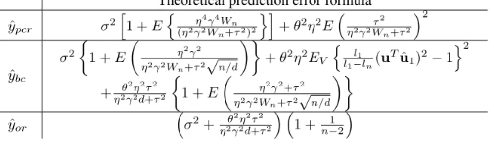
Table 1: Formulas for theoretical prediction error used in simulations (derived from Theorem 2 and Propositions 1-2). Expectations in theoretical prediction error expressions foryˆpcr andyˆbc were
computed empirically.
Theoretical prediction error formula ˆ ypcr σ2 h 1 +En η4γ4Wn (η2γ2W n+τ2)2 oi +θ2η2E τ2 η2γ2W n+τ2 2 ˆ ybc σ2 1 +E η2γ2 η2γ2Wn+τ2√n/d +θ2η2E V n l1 l1−ln(u Tu1)ˆ 2−1o2 +η2θγ22ηd2+τ2τ2 1 +E η2γ2+τ2 η2γ2Wn+τ2√n/d ˆ yor σ2+ θ2η2τ2 η2γ2d+τ2 1 + 1 n−2
and the theoretical prediction error for each method, Relative Error=
(Empirical PE)−(Theoretical PE) Empirical PE ×100%.
Table 2:d= 500. Prediction error foryˆpcr(PCR),yˆbc(Bias-corrected PCR), andyˆor(oracle).
Rel-ative error for comparing Empirical PE and Theoretical PE is given in parentheses. “NA” indicates that Theoretical PE values are unknown.
PCR Bias-corrected
PCR Oracle
n= 2 Empirical PE 18.7967 4.8668 1.5836
Theoretical PE (Relative Error) NA ∞ (∞) ∞ (∞)
n= 4 Empirical PE 6.4639 0.8023 0.3268
Theoretical PE (Relative Error) NA NA 0.3416 (4.53%)
n= 9 Empirical PE 1.4187 0.3565 0.2587
Theoretical PE (Relative Error) 1.2514 (11.79%) 0.2857 (19.86%) 0.2603 (0.62%)
n= 20 Empirical PE 0.4513 0.2732 0.2398
Theoretical PE (Relative Error) 0.2987 (33.81%) 0.2497 (8.60%) 0.2404 (0.25%) The results of the simulation study are summarized in Tables 2-3. Observe that yˆbc has smaller
empirical prediction error thanyˆpcrin every setting considered in Tables 2-3, andyˆbcsubstantially
outperformsyˆpcr in most settings. Indeed, the empirical prediction error foryˆbc whenn = 9is
smaller than that ofyˆpcr whenn = 20(for bothd = 500 andd = 5000); in other words, yˆbc
outperformsyˆpcr, even whenyˆpcr has more than twice as much training data. Additionally, the
empirical prediction error ofyˆbcis quite close to that of the oracle methodyˆor, especially whenn
is relatively large. These results highlight the effectiveness of the bias-corrected PCR methodyˆbcin
settings whereσ2andnare small,η2γ2/τ2is substantially larger than 0, anddis large.
Forn= 2,4, theoretical prediction error is unavailable in some instances. Indeed, while Proposition 2 and the discussion in Section 4 imply that ifn= 2, thenRV(ˆybc) =RV(ˆyor) =∞, we have not
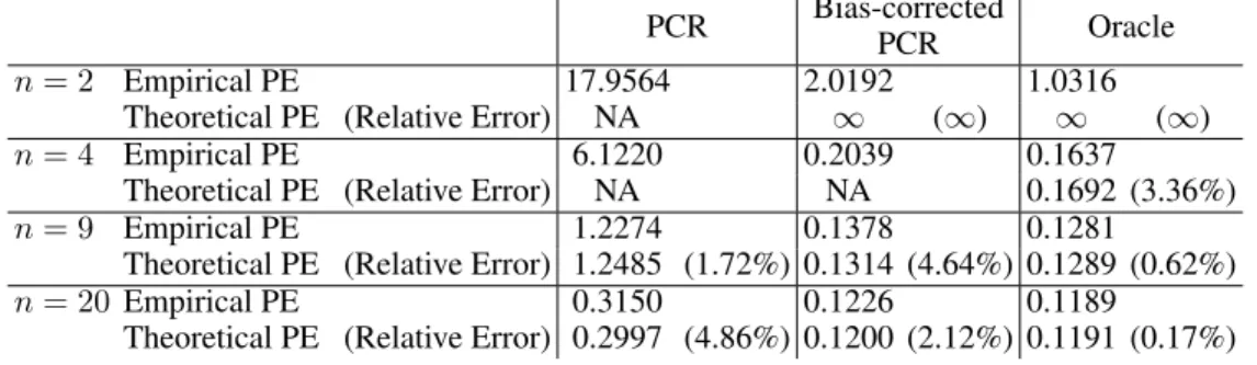
Table 3: d = 5000. Prediction error foryˆpcr (PCR),yˆbc (Bias-corrected PCR), andyˆor (oracle).
Relative error comparing Empirical PE and Theoretical PE is given in parentheses. “NA”’ indicates that Theoretical PE values are unknown.
PCR Bias-corrected
PCR Oracle
n= 2 Empirical PE 17.9564 2.0192 1.0316
Theoretical PE (Relative Error) NA ∞ (∞) ∞ (∞)
n= 4 Empirical PE 6.1220 0.2039 0.1637
Theoretical PE (Relative Error) NA NA 0.1692 (3.36%)
n= 9 Empirical PE 1.2274 0.1378 0.1281
Theoretical PE (Relative Error) 1.2485 (1.72%) 0.1314 (4.64%) 0.1289 (0.62%)
n= 20Empirical PE 0.3150 0.1226 0.1189
Theoretical PE (Relative Error) 0.2997 (4.86%) 0.1200 (2.12%) 0.1191 (0.17%)
pursued an expression forRV(ˆypcr)whenn= 2(it appears thatRV(ˆypcr)<∞); furthermore, the
approximations in Theorem 2 forRV(ˆypcr), RV(ˆybc)do not apply whenn= 4. In instances where
theoretical prediction error is available, is finite, andd= 500, the relative error between empirical and theoretical prediction error foryˆpcrandyˆbcranges from 8.60%-33.81%; ford= 5000, it ranges
from 1.72%-4.86%. Thus, the accuracy of the theoretical prediction error formulas tends to improve as d increases, as one would expect. Further improved measures of theoretical prediction error for yˆpcr andyˆbc could potentially be obtained by refining the approximations in Theorem 2 and
Proposition 1.
8
Discussion
In this article, we have proposed bias-corrected PCR for consistent one-shot learning in a simple latent factor model with continuous outcomes. Our analysis was motivated by problems in one-shot learning, as discussed in Section 1. However, the results in this paper may also be relevant for other applications and techniques related to high-dimensional data analysis, such as those involving reproducing kernel Hilbert spaces. Furthermore, our analysis sheds new light on PCR, a long-studied method for regression and prediction.
Many open questions remain. For instance, consider the semi-supervised setting, where additional unlabeled dataxn+1, ...,xN is available, but the corresponding yi’s are not provided. Then the
additionalx-data could be used to obtain a better estimate of the first principal componentuand perhaps devise a method whose performance is closer to that of the oracle procedureyˆor (indeed,
ˆ
yor may viewed as a semi-supervised procedure that utilizes an infinite amount of unlabeled data
to exactly identifyu). Is correction via inflation necessary in this setting? Presumably, bias-correction is not needed ifN is large enough, but can this be made more precise? The simulations described in the previous section indicate thatyˆbc outperforms the uncorrected PCR methodyˆpcr
in settings where twice as muchlabeleddata is available foryˆpcr. This suggests that role of
bias-correction will remain significant in the semi-supervised setting, where additional unlabeled data (which is less informative than labeled data) is available. Related questions involving transductive learning [26, 27] may also be of interest for future research.
A potentially interesting extension of the present work involves multi-factor models. As opposed to the single-factor model (1)-(2), one could consider a more generalk-factor model, whereyi =
hT
iθ+ξiandxi=Shi+i; herehi= (hi1, ..., hik)T ∈Rkis a multivariate normal random vector (ak-dimensional factor linkingyi andxi),θ = (θ1, ..., θk)T ∈Rk, andS =
√
d(γ1u1· · ·γkuk)
is ak×dmatrix, withγ1, ..., γk ∈Rand unit vectorsu1, ...,uk ∈ Rd. It may also be of interest to work on relaxing the distributional (normality) assumptions made in this paper. Finally, we point out that the results in this paper could potentially be used to develop flexible probit (latent variable) models for one-shot classification problems.
References
[1] L. Fei-Fei, R. Fergus, and P. Perona. One-shot learning of object categories.Pattern Analysis and Machine Intelligence, IEEE Transactions on, 28:594–611, 2006.
[2] R. Salakhutdinov, J.B. Tenenbaum, and A. Torralba. One-shot learning with a hierarchical nonparametric Bayesian model. JMLR Workshop and Conference Proceedings Volume 26: Unsupervised and Transfer Learning Workshop, 27:195–206, 2012.
[3] M.C. Frank, N.D. Goodman, and J.B. Tenenbaum. A Bayesian framework for cross-situational word-learning.Advances in Neural Information Processing Systems, 20:20–29, 2007.
[4] J.B. Tenenbaum, T.L. Griffiths, and C. Kemp. Theory-based Bayesian models of inductive learning and reasoning.Trends in Cognitive Sciences, 10:309–318, 2006.
[5] C. Kemp, A. Perfors, and J.B. Tenenbaum. Learning overhypotheses with hierarchical Bayesian models.
Developmental Science, 10:307–321, 2007.
[6] S. Carey and E. Bartlett. Acquiring a single new word. Proceedings of the Stanford Child Language Conference, 15:17–29, 1978.
[7] L.B. Smith, S.S. Jones, B. Landau, L. Gershkoff-Stowe, and L. Samuelson. Object name learning provides on-the-job training for attention.Psychological Science, 13:13–19, 2002.
[8] F. Xu and J.B. Tenenbaum. Word learning as Bayesian inference. Psychological Review, 114:245–272, 2007.
[9] M. Fink. Object classification from a single example utilizing class relevance metrics.Advances in Neural Information Processing Systems, 17:449–456, 2005.
[10] P. Hall, J.S. Marron, and A. Neeman. Geometric representation of high dimension, low sample size data.
Journal of the Royal Statistical Society: Series B (Statistical Methodology), 67:427–444, 2005.
[11] P. Hall, Y. Pittelkow, and M. Ghosh. Theoretical measures of relative performance of classifiers for high dimensional data with small sample sizes. Journal of the Royal Statistical Society: Series B (Statistical Methodology), 70:159–173, 2008.
[12] Y.I. Ingster, C. Pouet, and A.B. Tsybakov. Classification of sparse high-dimensional vectors. Philosoph-ical Transactions of the Royal Society A: MathematPhilosoph-ical, PhysPhilosoph-ical and Engineering Sciences, 367:4427– 4448, 2009.
[13] W.F. Massy. Principal components regression in exploratory statistical research.Journal of the American Statistical Association, 60:234–256, 1965.
[14] I.M. Johnstone. On the distribution of the largest eigenvalue in principal components analysis.Annals of Statistics, 29:295–327, 2001.
[15] D. Paul. Asymptotics of sample eigenstructure for a large dimensional spiked covariance model.Statistica Sinica, 17:1617–1642, 2007.
[16] B. Nadler. Finite sample approximation results for principal component analysis: A matrix perturbation approach.Annals of Statistics, 36:2791–2817, 2008.
[17] I.M. Johnstone and A.Y. Lu. On consistency and sparsity for principal components analysis in high dimensions.Journal of the American Statistical Association, 104:682–693, 2009.
[18] S. Jung and J.S. Marron. PCA consistency in high dimension, low sample size context.Annals of Statis-tics, 37:4104–4130, 2009.
[19] S. Lee, F. Zou, and F.A. Wright. Convergence and prediction of principal component scores in high-dimensional settings.Annals of Statistics, 38:3605–3629, 2010.
[20] Q. Berthet and P. Rigollet. Optimal detection of sparse principal components in high dimension. arXiv preprint arXiv:1202.5070, 2012.
[21] S. Jung, A. Sen, and J.S Marron. Boundary behavior in high dimension, low sample size asymptotics of PCA.Journal of Multivariate Analysis, 109:190–203, 2012.
[22] Z. Ma. Sparse principal component analysis and iterative thresholding.Annals of Statistics, 41:772–801, 2013.
[23] C. Stein. Inadmissibility of the usual estimator for the mean of a multivariate normal distribution. In
Proceedings of the Third Berkeley Symposium on Mathematical Statistics and Probability, volume 1, pages 197–206, 1955.
[24] R. Tibshirani. Regression shrinkage and selection via the lasso. Journal of the Royal Statistical Society. Series B (Methodological), 58:267–288, 1996.
[25] T. Hastie, R. Tibshirani, and J. Friedman.The Elements of Statistical Learning: Data Mining, Inference, and Prediction. Springer, 2nd edition, 2009.
[26] V.N. Vapnik.Statistical Learning Theory. Wiley, 1998.
[27] K.S. Azoury and M.K. Warmuth. Relative loss bounds for on-line density estimation with the exponential family of distributions.Machine Learning, 43:211–246, 2001.