Technical efficiency and technology gaps in beef cattle production systems in Kenya: A stochastic metafrontier analysis
David Jakinda Otieno, Lionel Hubbard and Eric Ruto
School of Agriculture, Food and Rural Development, Newcastle University, NE1 7RU, UK Contact: [email protected]
A contributed paper prepared for presentation at the 85th annual Conference of the Agricultural Economics Society (AES)
18 – 20 April 2011 University of Warwick, UK
Abstract
In this study the stochastic metafrontier method is used to investigate technical efficiency and technology gaps across three main beef cattle production systems in Kenya. Results show that there is significant inefficiency in nomadic and agro-pastoral systems. Further, in contrast with ranches, these two systems were found to have lower technology gap ratios. The average pooled technical efficiency was estimated to be 0.69, which suggests that there is considerable scope to improve beef production in Kenya.
Key words: Technical efficiency; technology gap; beef cattle; production systems; stochastic metafrontier; Kenya.
JEL classifications: D24; O32; Q18. 1. Introduction
The analysis of efficiency originated from the seminal work of Farell (1957), who defined technical efficiency (TE) as the ability of a firm to produce maximum output from a given level of inputs, or achieve a certain output threshold using a minimum quantity of inputs, under a given technology. Measurement of TE provides useful insights that may enhance decision-making on optimal use of resources and effective capacity utilisation. As noted by Abdulai and Tietje (2007), analysis of TE can also deliver important information on competitiveness of farms and their potential for increasing productivity.
There is an extensive literature on TE analysis on crop, dairy and mixed crop-livestock enterprises. However, published research on TE of beef cattle farms is very limited; exceptions include Barnes (2008), Ceyhan and Hazneci (2010), Featherstone et al. (1997), Fleming et al. (2010), Hadley (2006) and Rakipova et al. (2003). In Kenya, where the livestock sector contributes about 42% of agricultural output (KIPPRA, 2009), no study has analysed TE in beef cattle
production. The few TE studies undertaken in Kenya mainly focus on crops (e.g., Liu and Myers, 2009 and Nyagaka et al., 2010) and dairy farms (e.g., Kavoi et al., 2010).
Generally, crop and livestock enterprises in Kenya are characterised by stagnating or declining productivity, partly due to high unit cost of production and inability by farmers to afford high-yielding farm technologies (KIPPRA, 2009). Beef cattle are mainly reared on natural pastures, with supplementation from improved pastures and purchased feeds such as concentrates from cereals and legumes fodder. However, pasture supply fluctuates due to seasonal rains, while the quality of commercial feeds is often compromised in the supply chain (Republic of Kenya, 2007). Further, public funds allocated to livestock development are relatively low (generally less than 10% of the annual national development expenditure), despite the contribution of livestock to livelihood sustenance (Otieno, 2008). Moreover, there is limited investment in the provision of livestock inputs such as veterinary and extension services, or market infrastructure. Public agricultural research and extension services are relatively limited in scope due to inadequate number of trained personnel (Oluoch-Kosura, 2010). Private extension providers tend to focus mainly on high value export crops (e.g., coffee, tea, horticulture) and dairy (Muyanga and Jayne, 2006); service provision to beef cattle farmers is very limited. Further, in remote rural areas where public veterinary services are scarce, livestock disease control is mainly dealt with by community-based animal health service providers (Irungu et al., 2006), some of whom lack professional veterinary skills. Livestock marketing is mainly handled by the private sector, while the government provides regulatory services. The government also operates an export-abattoir (Kenya Meat Commission – KMC), but at less than half capacity due to dilapidated processing equipment (Matete et al., 2010). These issues might have a considerable bearing on farmers’ production decisions and efficiency. Against this backdrop, the present study investigates TE and technology gaps in Kenya’s main beef cattle production systems: nomadic pastoralism, agro-pastoralism and ranches.
Nomadic pastoralism and agro-pastoralism contribute about 65% of total beef output in Kenya, while the rest is obtained from ranches and a small proportion of dairy-culls. About 80% of land in Kenya is arid and semi-arid, and it is estimated that over 60% of livestock is kept by pastoralists in these areas. The livestock provide employment to 90% of the population in those areas and contribute 95% of their income (KIPPRA, 2009; Otieno, 2008). Nomadic pastoralists (also referred to as nomads) typically have temporary abodes and migrate seasonally with cattle and other livestock in search for pasture and water. They are less commercialised, but derive a relatively large share of their livelihood from cattle and other livestock. In contrast, the agro-pastoralists are sedentary; they keep cattle and other livestock, besides cultivating crops, and are relatively commercialised. Ranches are purely commercial livestock enterprises and may also grow a few crops for use as on-farm fodder or for sale. They mainly use controlled grazing on their private land,
and purchased supplementary feeds, in contrast to both the nomads and agro-pastoralists who generally depend on open grazing, with limited use of purchased feeds. Investigating the TE of various cattle production systems in Kenya should provide insights on how to better integrate livestock development in the national economic agenda, as well as guidance to farmers on resource allocation.
We use the parametric stochastic frontier approach (SFA) (Aigner et al., 1977; Meeusen and van den Broeck, 1977) to investigate TE in individual production systems. The SFA has a two-sided error term composed of technical inefficiency and random statistical noise. By separating the effect of stochastic noise from that of inefficiency, the SFA allows hypotheses to be tested regarding the production structure and extent of inefficiency (Coelli et al., 2005), unlike alternative non-parametric approaches such as data envelopment analysis (DEA) proposed by Charnes et al. (1978). In order to permit comparison of TE across different production systems, we apply the stochastic metafrontier proposed by Battese and Rao (2002). This involves use of the SFA to estimate parameters of various groups or production systems and then likelihood ratio (LR) tests to investigate differences between the individual groups and the pooled sample; where LR tests show differences, an optimisation problem is solved to provide the ‘best’ frontier (technology-wise) to which all group frontiers can be compared. The stochastic metafrontier technique enables estimation of technology gaps for different groups and accommodates both cross-sectional and panel data, and therefore is preferred to alternative methods such as random and fixed parameter frontier models (Greene, 2005) and the stochastic latent class frontier (Orea and Kumbhakar, 2004; Alvarez and Corral, 2010) which are suited to panel data estimation. Other approaches involving classification of the data using a priori information (e.g., production systems) and estimation of frontiers for separate groups (Newman and Mathews, 2006) would not adequately explain within-group variations.
Empirical applications of the stochastic metafrontier are still few, but include estimation of TE and technology gaps for different agricultural enterprises (e.g., Boshrabadi et al., 2008; Chen and Song, 2008; O’Donnell et al., 2008; Villano et al., 2010; Wang and Rungsuriyawiboon, 2010). This method has also been used to assess efficiency differences in other sectors, for instance garment firms (Battese et al., 2004), electronic firms (Yang and Chen, 2009), and electricity distribution firms (Huang et al., 2010). The present study is the first to apply the stochastic metafrontier to investigate TEs and technology gaps in various beef cattle production systems.
The rest of the paper is organised as follows: the stochastic metafrontier analytical framework is explained in section 2, while section 3 describes the data and empirical estimation. Results are presented and discussed in section 4. Finally, some conclusions are highlighted in section 5.
2. Stochastic metafrontier analytical framework
Following Aigner et al. (1977), Meeusen and van den Broeck (1977) and Battese and Rao (2002), suppose we have k groups or production systems in the cattle industry:
(
nk k) (
nk nk)
kn f X v u
Q = ,β exp − (1)
where Qnkis the output of the nth farm in the kth production system;
X denotes a vector of inputs used by the farm; is a vector of parameters to be estimated;
v represents statistical noise assumed to be independently and identically distributed (IID) as a normal random variable with zero mean and variance given by 2
v
σ , i.e., v~
( )
0, 2v
N σ ; while u is a non-negative random variable assumed to capture technical inefficiency in production.
The u is assumed to be IID half-normal, i.e., u~|
( )
0, 2 | uN σ . Following Battese and Corra (1977), the variation of output from the frontier due to technical inefficiency is defined by a parameter ( ) given by:
2 2 σ σ γ = u such that 0≤γ ≤1 (2) where 2 = 2u+ 2v.
Although u can assume exponential or other distributions, the half-normal distribution is preferred for parsimony because it entails less computational complexity (Coelli et al., 2005). Equation (1) can be estimated through maximum likelihood. The TE of the nth farm with respect to the kth production system frontier is obtained as:
(
) ( )
(
nk)
nk k nk nk nk f X v u Q TE = =exp − exp ,β (3)Equation (3) allows comparison of farms operating with similar technologies. However, farms in different environments (e.g., production systems) do not always have access to the same technology. Assuming similar technologies when they actually differ across farms might result in erroneous measurement of efficiency by mixing technological differences with technology-specific inefficiency (Tsionas, 2002). Technologies in this study comprise the type of cattle breed, breeding method and feeding methods. Variations in output between production systems due to technology differences can be captured by using the metafrontier, which is considered to be a smooth or common technology frontier that envelops the deterministic components of the group stochastic frontiers (Battese and Rao, 2002; Battese et al., 2004). The metafrontier explains deviations
between observed outputs and the maximum possible explained output levels in the group frontiers. Following O’Donnell et al. (2008), the stochastic metafrontier equation can be expressed as:
(
, *)
* n β
n f X
Q = n = 1,2, … N (4)
where (f(.)) is a specified functional form; Qn* is the metafrontier output; and * denotes the vector
of metafrontier parameters that satisfy the constraints:
(
Xn) (
f Xn k)
f ,β* ≥ ,β , for all k = 1,2, … K (5)
According to (5), the metafrontier function dominates all the group frontiers. In order to satisfy this condition, an optimization problem is solved, where the sum of absolute deviations (or sum of squared deviations) of the metafrontier values from the group frontiers is minimised. The optimization problem is usually expressed as (Battese et al., 2004):
(
)
(
)
(
n)
(
n k)
k n N n n X f X f t s X f X f β β β β , ln * , ln . . | , ln * , ln | min 1 ≥ − = (6)The standard errors of the estimated metafrontier parameters can be obtained through bootstrapping or simulation methods.
In terms of the metafrontier, the observed output for the nth farm in the kth production system
(measured by the stochastic frontier in (1)) can be expressed as:
(
)
n( )
nk n k n nk nk f X v X f X f u Q . ( , *)exp *) , ( ) , ( . exp * β β β − = (7)where (recall from (3) that, exp(-unk) = TEnk) the middle term in (7) represents the technology gap
ratio (TGR), whose value is bounded between zero and one:
(
)
(
, *)
, ββ n k n n X f X f TGR = (8)The TGR measures the ratio of the output for the frontier production function for the kth
group or production system relative to the potential output defined by the metafrontier, given the observed inputs (Battese and Rao, 2002; Battese et al., 2004). Values of TGR closer to 1 imply that a farm in a given production system is producing nearer to the maximum potential output given the technology available for the whole industry. For instance, a value of 0.97 suggests that the farm produces on average 97% of the potential output, assuming all farmers use a common technology.
The notion of TGR defined in (8) depicts the gap between the production frontier for a particular production system or group frontier and the metafrontier (Battese et al., 2004). However, a confusion of terminology arises because an increase in the (technology gap) ratio implies a
decrease in the gap between the group frontier and the metafrontier. Further, it is important to expand the definition of TGR to account for constraints placed on the potential output by the environment, and interactions between the production technology and the environment. Accordingly, recent literature uses meta-technology ratio (MTR) or environment-technology gap ratio (ETGR), rather than TGR (Boshrabadi et al, 2008; O’Donnell et al., 2008). Subsequently, the TGR is referred to as MTR in this study. The MTR considers environmental limitations on the production technology. Generally, the potential for productivity gains from use of a given technology (e.g., cattle breed or breeding method) varies across production systems, depending on natural environmental constraints such as rainfall distribution (which determine feed quality and availability). Further, human influences on the production environment, for example, skewed distribution of extension services, and veterinary drugs and advisory services, might affect the ability of farmers to achieve the highest production potential of a given technology.
The TE of the nth farm relative to the metafrontier (TE*n) is the ratio of the observed output
for the nth farm relative to the metafrontier output, adjusted for the corresponding random error such that:
(
n) ( )
nk nk n f X v Q TE exp * , * β = (9)Following (3), (7) and (8), the TE*n can be expressed as the product of the TE relative to the
stochastic frontier of a given production system and the MTR: n
nk n TE MTR
TE *= . (10)
3. Data and empirical estimation
3.1. Sampling and data collection
The study uses survey data from four sites (Kajiado, Kilifi, Makueni and Taita Taveta districts) that are representative of the three beef cattle production systems in Kenya: nomadic pastoralism, agro-pastoralism and ranches. Generally, Kenya is divided into seven agro-climatic zones based on moisture index, i.e., the annual rainfall as a percentage of potential evaporation. Places with moisture index above 50% are classified as zones I, II and III, and are considered to have high potential for agriculture. The areas sampled in the study represent different agro-ecological zones, but are contiguous, hence logistically more accessible. Kajiado is in zone VI, which includes semi-arid to semi-arid rangelands with mean annual rainfall of 300–800mm, and a moisture index of 25–40% (Orodho, 2002). However, rainfall in Kajiado is highly variable within and between years, and there are frequent droughts in the area (Thornton et al., 2007). Due to the relatively drier and hot weather in Kajiado, the area is mostly characterised by nomadic pastoralism. Kilifi is a semi-humid region
(zone III) with an annual rainfall between 760–1,300mm and moisture index of about 65%. The area is mainly characterised by ranches and tree-crops including coconuts and mangoes. Makueni is a semi-arid area (zone V), with average rainfall of 500–760mm and 40% moisture index annually. In this area, there is some dry-land irrigated crop farming focusing on fruits and vegetables. Finally, Taita Taveta is semi-humid to semi-arid (zone IV). On average, this site is estimated to have 500– 750mm of annual rainfall and about 50% moisture index. Both Makueni and Taita Taveta are characterised by more agro-pastoralists than nomads and ranchers (Republic of Kenya, 2007 & 2008).
A multi-stage cluster (area) sampling approach (Horppila and Peltonen, 1992) was used. Within the four districts, smaller administrative units (divisions) were randomly selected from lists of all divisions in these districts, taking into account the general distribution of cattle in the study area. Subsequent stages involved a random selection of a sample of locations, from which a number of smaller units (sub-locations) were selected. The primary sampling units for the survey were therefore 40 sub-locations. Systematic random sampling was used to select individual respondents for interview during the survey. During the survey, nomads were selected from Kajiado, agro-pastoralists from Makueni and Taita Taveta, and ranchers from Kilifi.
A structured questionnaire was used to collect data on: relative importance of cattle and other enterprises to household income; cattle inventory in the past twelve months; production inputs such as feeds, labour, veterinary supplies and advisory services, and fixed inputs; cattle breeding methods; access to extension and market services; and household socio-demographic characteristics. With the assistance of local experienced interviewers, who were trained prior to the survey, the questionnaire was piloted, revised and then administered through face-to-face interviews of farmers between July and December 2009. A random route procedure (for example first left, next right, and so on) was followed by the interviewers to select every fifth or tenth farmer, in sparsely or densely populated sub-locations, respectively. In total, 313 farmers including 66 ranchers, 110 nomads and 137 agro-pastoralists were interviewed.
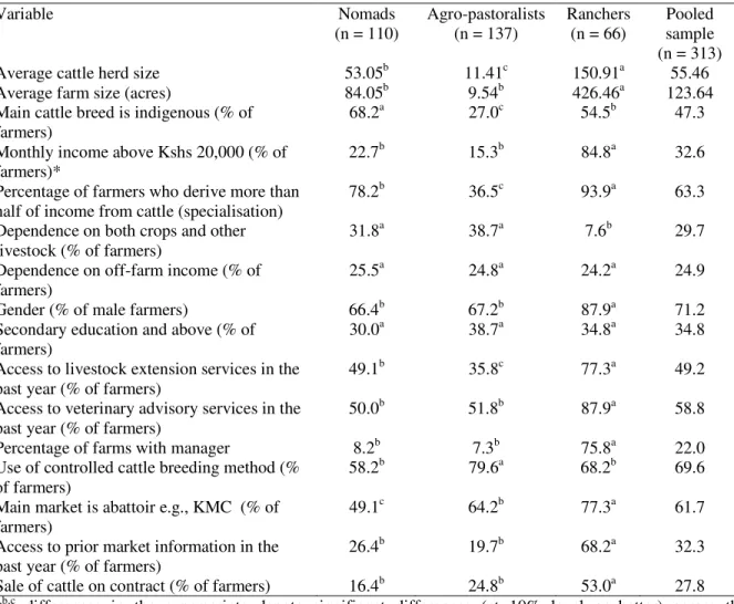
Some of the sample characteristics are shown in Table 1. Ranchers on average have larger herds and farms than the nomads and agro-pastoralists. Both nomads and ranchers tend to keep indigenous (local) cattle breeds such as the Zebu and Boran, which are relatively more adapted to dry and hot areas (e.g., Kajiado and Kilifi) where most farmers in the two systems live. In contrast, the agro-pastoralists have a majority of exotic and crossbreeds. The ranchers have significantly higher average monthly household incomes and, in common with the nomads, depend more heavily on cattle as the main source of income. Only a quarter of farmers in the three systems depend on off-farm income. Two-thirds or more of farmers in all the production types are male, with ranchers
having less than a quarter of females. Across the three production systems, less than 40% have formal education at the secondary level or above.
Ranchers benefit from relatively better access to livestock extension and veterinary advisory services, and most of them have farm managers. A higher proportion of agro-pastoralists use controlled cattle breeding. This is consistent with the observation that the more commercially-oriented farmers (i.e., ranchers and agro-pastoralists) prefer cattle breeding strategies that target market and/or profitability requirements, e.g., faster growth and higher gains in live weight, while the relatively less-commercialised nomads mainly focus on cattle survival traits such as drought resistance, hardiness and disease tolerance (Gamba, 2006). Generally, more than half of farmers sell cattle to abattoirs such as the KMC, while the rest sell in open air markets and other outlets. Only one third of farmers (mostly ranchers) have access to prior market information and sell on contract.
Table 1: Sample characteristics from the survey
Variable Nomads
(n = 110) Agro-pastoralists (n = 137) Ranchers (n = 66) Pooled sample (n = 313) Average cattle herd size 53.05b 11.41c 150.91a 55.46
Average farm size (acres) 84.05b 9.54b 426.46a 123.64
Main cattle breed is indigenous (% of
farmers) 68.2
a 27.0c 54.5b 47.3
Monthly income above Kshs 20,000 (% of
farmers)* 22.7
b 15.3b 84.8a 32.6
Percentage of farmers who derive more than
half of income from cattle (specialisation) 78.2
b 36.5c 93.9a 63.3
Dependence on both crops and other
livestock (% of farmers) 31.8
a 38.7a 7.6b 29.7
Dependence on off-farm income (% of
farmers) 25.5
a 24.8a 24.2a 24.9
Gender (% of male farmers) 66.4b 67.2b 87.9a 71.2
Secondary education and above (% of
farmers) 30.0
a 38.7a 34.8a 34.8
Access to livestock extension services in the
past year (% of farmers) 49.1
b 35.8c 77.3a 49.2
Access to veterinary advisory services in the
past year (% of farmers) 50.0
b 51.8b 87.9a 58.8
Percentage of farms with manager 8.2b 7.3b 75.8a 22.0
Use of controlled cattle breeding method (%
of farmers) 58.2
b 79.6a 68.2b 69.6
Main market is abattoir e.g., KMC (% of
farmers) 49.1
c 64.2b 77.3a 61.7
Access to prior market information in the
past year (% of farmers) 26.4
b 19.7b 68.2a 32.3
Sale of cattle on contract (% of farmers) 16.4b 24.8b 53.0a 27.8 a,b,c differences in the superscripts denote significant differences (at 10% level or better) across the
production systems.
3.2. Measurement of variables
In studies of this kind, beef output would be considered as the dependent variable, while a number of inputs (e.g., herd size, feeds, veterinary costs, fixed costs etc.) are included as regressors in the model. However, due to measurement difficulties, previous studies have used proxy variables, for example, value-added (Featherstone et al., 1997) or physical weights of cattle (Rakipova et al., 2003). As such data are not available in the present study, we follow the revenue approach recently applied in the literature (Hadley, 2006; Abdulai and Tietje, 2007; and Gaspar et al., 2009), and define output as:
t yp Q R r k n( ) = (11)
where Qn(k) is the annual value of beef cattle output of the nth farm in the kthproduction system
(measured in Kenya shillings; Kshs); r denotes any of the three forms of cattle output considered, i.e., current stock, sales or uses for other purposes in the past twelve-month period; y is the number of beef cattle equivalents1; p is the current price of existing stock or average price for cattle sold/used during the past twelve months; and t is the average maturity period for beef cattle in Kenya, which is four years (Republic of Kenya, 2008).
The beef cattle herd size was computed as the average number of cattle kept in the past twelve months, adjusted with the conversion factors. In order to capture the approximate share of feeds from different sources, the quantities of purchased and non-purchased (or on-farm) feeds were first adjusted with the average annual number of dry and wet months, respectively, in each district (Lukuyu et al., 2009; Orodho, 2002). Assuming one price in a given locality (Chavas and Aliber, 1993), average feed prices were computed using prices from district annual reports and recent surveys (e.g., Lukuyu et al., 2009). Both purchased and non-purchased feeds were then converted to improved feed equivalents by multiplying the respective feed quantities by the ratio of their prices (or opportunity costs) to the average per unit price of improved fodder. Thus, the total annual improved feed equivalent was computed as:
(
)
{
ϕ pf *d +s(
np*w)}
(12)where; and s denote, respectively, the ratio of prices of purchased and non-purchased feed to that of improved fodder; pf and np represent the average quantities of purchased and non-purchased
feeds, respectively, in kilogrammes per month; d is the approximate number of dry months (when
1 Beef cattle equivalents were computed by multiplying the number of cattle of various types by conversion factors
(Hayami and Ruttan, 1970; O’Donnell et al., 2008). Following insights from focused group discussions with key informants in the livestock sector in Kenya, the conversion factors were calculated as the ratio of average slaughter weight of different cattle types to the average slaughter weight of a mature beef bull. The average slaughter weight of mature bull, considered to be suitable for beef in Kenya, is 159 kg (FAO, 2005). The estimated conversion factors were: 0.2, 0.6, 0.75, 0.8 and 1, for calves, heifers, cows, steers and bulls, respectively.
purchased feeds are mainly used), while w is the length of the wet season (when farmers mostly use on-farm or non-purchased feeds) in a particular area.
Depreciation costs on fixed inputs were based on the straight line method, assuming a 10% salvage value following discussions with relevant officials in the Ministry of Livestock Development. The depreciable value of an asset was based on the proportion of time that it was used in the cattle enterprise. Labour costs comprise both paid and unpaid labour; the latter valued using the average minimum farm wage. The labour costs were adjusted with the share of cattle income in household income. Similar adjustments were applied to other incidental variable costs, such as fuel and electricity bills2.
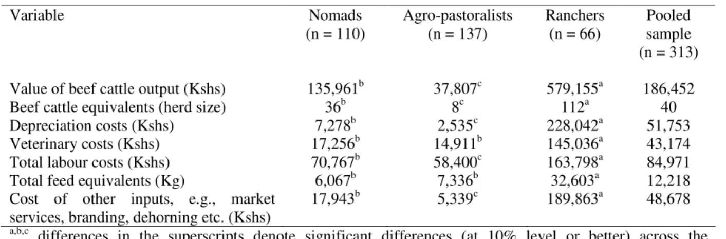
The data on the main production variables for the beef cattle enterprise are summarised in Table 2. On average, ranchers use more inputs and produce the highest output. Nomads and agro-pastoralists use significantly lower amounts of improved feeds and invest less in professional veterinary services than ranchers. Consistent with their less-sedentary nature, the nomads use the least amount of on-farm feeds (which might be from naturally-growing pasture in their temporary abodes or possibly donations from sedentary farmers; there is no evidence to indicate that nomads invest in fodder cultivation). However, nomads have higher depreciation costs than agro-pastoralists, because almost all of them possess portable cattle equipment such as dip sprayer, chaff cutter, dehorning and castration equipment.
Table 2: Average annual output and inputs
Variable Nomads
(n = 110) Agro-pastoralists (n = 137) Ranchers (n = 66) sample Pooled (n = 313) Value of beef cattle output (Kshs) 135,961b 37,807c 579,155a 186,452
Beef cattle equivalents (herd size) 36b 8c 112a 40
Depreciation costs (Kshs) 7,278b 2,535c 228,042a 51,753
Veterinary costs (Kshs) 17,256b 14,911b 145,036a 43,174
Total labour costs (Kshs) 70,767b 58,400c 163,798a 84,971
Total feed equivalents (Kg) 6,067b 7,336b 32,603a 12,218
Cost of other inputs, e.g., market
services, branding, dehorning etc. (Kshs) 17,943
b 5,339c 189,863a 48,678 a,b,c differences in the superscripts denote significant differences (at 10% level or better) across the
production systems.
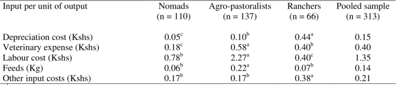
Partial input shares are computed to provide a priori indication of differences in production technologies across the three production systems (Table 3). Generally, the ratios of expenses on veterinary services and labour in total value of output are relatively larger than those of other
2 In addition, land was measured as farm size (adjusted with the share of cattle income in household income). However,
it was found to be highly correlated with feeds in agro-pastoralism. Further, it was difficult to establish owner-occupancy on land with respect to cattle production for nomads. Consequently, the use of imputed land rent as an input (see for example, Hadley, 2006) was not suitable for this study.
inputs3. Agro-pastoralists have the highest share of veterinary cost and feeds per unit of output. Depreciation and cost of other inputs (e.g., market services) per unit of output are highest in ranches, while nomads have the lowest per unit veterinary expenses. Finally, the ranchers use relatively less feeds per unit output. This suggests perhaps, that the ranchers keep relatively better cattle in terms of feed conversion. Considering these differences, farmers across the three production systems might be expected to have different levels of efficiency.
Table 3: Partial input shares in output
Input per unit of output Nomads
(n = 110) Agro-pastoralists (n = 137) Ranchers (n = 66) Pooled sample (n = 313) Depreciation cost (Kshs) 0.05c 0.10b 0.44a 0.15
Veterinary expense (Kshs) 0.18c 0.58a 0.40b 0.40
Labour cost (Kshs) 0.78b 2.27a 0.40c 1.35
Feeds (Kg) 0.06b 0.22a 0.07b 0.14
Other input costs (Kshs) 0.17b 0.17b 0.38a 0.21
a,b,c Differences in the superscripts denote significant differences (at 10% level or better) across the
production systems.
3.3. Empirical estimation
The parameters of the stochastic frontiers for the production systems were estimated using the Cobb-Douglas specification4:
) ( ) ( 4 1 ( ) ( ) ) ( 0 ) ( ln ln nk nk i ik nik k k n X v u Q = + + − = β β (13)
where Qn(k) is the annual value of beef cattle output;
Xni represents a vector of inputs where Xn1 is the beef herd size, Xn2 is feed equivalent and Xn3 is the
cost of veterinary services, while Xn4 is a Divisia index calculated as (Boshrabadi et al., 2008)5:
∏
= = 31 ( ) ) ( 4k i nik n C ni X α (14)where αni(k)represents the share of the ith input in the total cost for the nth farm in the kth production system;
3 The study found that a relatively higher proportion of labour cost in the pooled sample and for nomads and
agro-pastoralists, comprise imputed cost of unpaid labour. Due to this, the total cost of labour for agro-pastoralists and in the pooled sample is higher than average value of output.
4 A likelihood ratio (LR) test (Coelli et al., 2005) with an LR statistic of 3.58 compared with the chi-square critical
value of 18.31 at 5% level and 10 degrees of freedom did not support rejection of the null hypothesis that the Cobb-Douglas model provided a better fit to the data than an alternative translog model.
5 The Divisia index is a proxy variable used to possibly account for the effects of inputs that were not found to be
individually statistically significant (e.g., depreciation, labour etc.). Initially, the model was estimated with depreciation, labour and other costs as separate inputs but these were insignificant though with the expected positive sign, and were consequently consolidated into the Divisia index to improve the model fit.
Cn1(k) = depreciation costs, insurance and taxes on farm buildings, machinery and equipment (Kshs);
Cn2(k) = cost of labour (Kshs);
Cn3(k) = other costs, e.g. fuel, electricity, hire/maintenance of machinery, market services, purchase
of ropes, branding etc. (Kshs);
u denotes inefficiency, while v represents statistical noise.
The log likelihood for the half-normal model can be expressed as (Greene, 2003):
(
)
[
(
)
]
= = − − Φ + − − Π − = N n n n N n n n X Q X Q n n L 1 ' 2 1 ' log 2 1 2 log 2 log log θ θ ξ λθ ξ (15) where σ θ = 1 , ξ =θβ , v u σ σ λ= ,(
2 2)
v u σ σσ = + and Φ
()
. is the probability density function of the standard normal distribution.The parameters of the stochastic frontiers were obtained by maximising the log likelihood function (15) using FRONTIER version 4.1c software (Coelli, 1996), while the metafrontier in (6) was estimated in SHAZAM version 10 software (Whistler et al., 2007) following codes adapted from O’Donnell et al. (2008).
4. Results and discussion
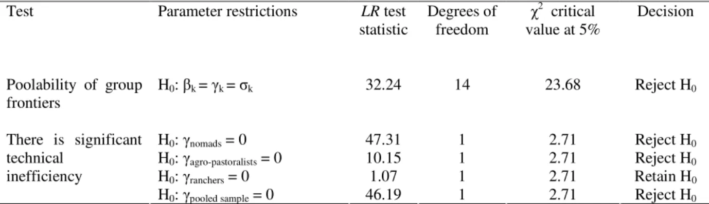
Various hypotheses are tested to establish the model fit (Table 4). The null hypothesis on poolability of the group frontiers is rejected, suggesting that there are significant differences in the input parameters, TE scores and random variations across the three production systems. This implies that differences exist in the production technology and environment, which justifies estimation of a metafrontier (Battese and Rao, 2002; Battese et al., 2004). The gamma ( ) test shows that there is significant technical inefficiency in the pooled frontier and group frontiers for nomads and agro-pastoralists, but less so for ranchers (Table 4).
Table 4: Hypothesis tests on the production structure Test Parameter restrictions LR test
statistic Degrees of freedom
2 critical value at 5% Decision Poolability of group frontiers H0: k = k = k 32.24 14 23.68 Reject H0 H0: nomads = 0 47.31 1 2.71 Reject H0 H0: agro-pastoralists = 0 10.15 1 2.71 Reject H0 H0: ranchers = 0 1.07 1 2.71 Retain H0 There is significant technical inefficiency
H0: pooled sample = 0 46.19 1 2.71 Reject H0
Notes: The hypothesis test involving a zero restriction on the gamma ( ) parameter follows a mixed chi-squareddistribution (i.e., joint test of equality and inequality, since the alternative hypothesis H1 is stated as
0 1). Following Coelli and Battese (1996), the critical value for this distribution is obtained from the statistical table of Kodde and Palm (1986).
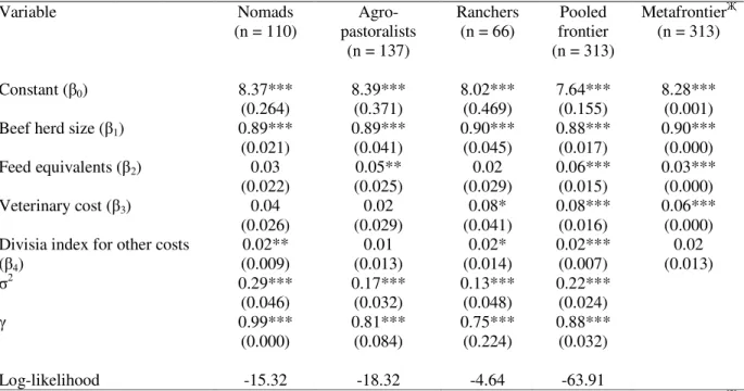
Consistent with assumed producer rationality (Coelli et al., 2005), the estimated input parameters are all positive at the sample mean (Table 5). Thus, as expected for a continuously differentiable production function, the elasticities fulfil the regularity condition of monotonicity (Sauer et al., 2006). The pooled sample results show that an increase in the application of any of the inputs would significantly increase output. Herd size is significant across the three production systems, while improved feeds are only significant in the agro-pastoralist system. Results suggest that only the ranchers derive significant returns from investment in professional veterinary management. This is to be expected, because most ranchers sell cattle to high premium abattoirs and export-oriented market outlets (e.g., the KMC) on contracts (see Table 1), which are usually characterised by stringent requirements on disease-free status. Sales contracts are important in enabling farmers to obtain steady and high income through an assured market, and reduce input and output price risks (MacDonald et al., 2004). Increased expenditure on other inputs (captured by the
Divisia index) would lead to significantly higher output in both nomadic and ranch systems. As expected for a ‘smooth envelope’ curve (Battese and Rao, 2002), the metafrontier parameters are generally similar to average values of the group frontier parameters.
14 Table 5: Stochastic frontier and metafrontier parameter estimates
Variable Nomads (n = 110) pastoralists Agro-(n = 137) Ranchers (n = 66) frontier Pooled (n = 313) Metafrontier (n = 313) Constant ( 0) 8.37*** (0.264) 8.39*** (0.371) 8.02*** (0.469) 7.64*** (0.155) 8.28*** (0.001) Beef herd size ( 1) 0.89***
(0.021) 0.89*** (0.041) 0.90*** (0.045) 0.88*** (0.017) 0.90*** (0.000) Feed equivalents ( 2) 0.03
(0.022) (0.025) 0.05** (0.029) 0.02 0.06*** (0.015) 0.03*** (0.000) Veterinary cost ( 3) 0.04
(0.026) (0.029) 0.02 (0.041) 0.08* 0.08*** (0.016) 0.06*** (0.000) Divisia index for other costs
( 4) 0.02** (0.009) (0.013) 0.01 (0.014) 0.02* 0.02*** (0.007) (0.013) 0.02 2 0.29*** (0.046) 0.17*** (0.032) 0.13*** (0.048) 0.22*** (0.024) 0.99*** (0.000) 0.81*** (0.084) 0.75*** (0.224) 0.88*** (0.032) Log-likelihood -15.32 -18.32 -4.64 -63.91
Notes: Standard errors are shown in parentheses. Statistical significance levels: ***1%; **5%; *10%. standard errors for metafrontier parameters were computed through bootstrapping (Freedman and Peters, 1984).
In addition to monotonicity, regularity conditions require that second order derivatives of production parameters (i.e., slope of the marginal physical product, MPP, curve) should be negative (Sauer et al., 2006). This is fulfilled for all inputs (though with an insignificant parameter for herd size), implying that farmers are rational in use of inputs (Table 6).
Table 6: Second-order derivatives of production parameters Change in variable Nomads
(n = 110) Agro-pastoralists (n = 137) Ranchers (n = 66) Pooled sample (n = 313) Beef herd size
( MPP1) -0.14 (1.47) (1.08) -0.09 (1.56) -0.19 (0.042) -0.002 Feed equivalents ( MPP2) -0.29*** (3.17) -0.29*** (3.45) -0.37*** (3.15) -0.18*** (3.18) Veterinary cost ( MPP3) -0.38*** (4.21) -0.50*** (6.65) -0.36*** (3.10) -0.17*** (3.11) Divisia index for other
costs ( MPP4)
-0.38***
(4.24) -0.53*** (7.18) -0.39*** (3.42) -0.15** (2.64) Notes: statistical significance levels: ***1%; **5%; *10%. Absolute values of the corresponding t-ratios are shown in parentheses.
The significance of 2 and the gamma ( ) parameter (see Table 5) indicate, respectively, that the models are stochastic (rather than deterministic) and exhibit technical inefficiency. Furthermore,
as shown in Table 7, the shortfall of all mean TE scores from 1 confirms the presence of technical inefficiency6. This implies that there is scope to improve efficiency in the utilisation of resources.
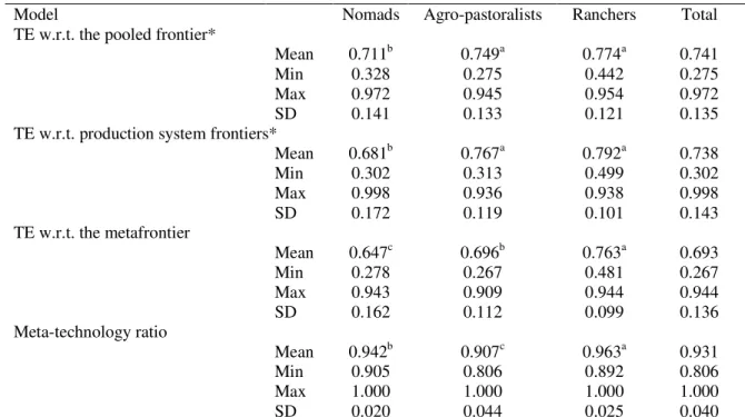
Table 7: Technical efficiency and meta-technology ratios
Model Nomads Agro-pastoralists Ranchers Total TE w.r.t. the pooled frontier*
Mean 0.711b 0.749a 0.774a 0.741
Min 0.328 0.275 0.442 0.275 Max 0.972 0.945 0.954 0.972 SD 0.141 0.133 0.121 0.135 TE w.r.t. production system frontiers*
Mean 0.681b 0.767a 0.792a 0.738 Min 0.302 0.313 0.499 0.302 Max 0.998 0.936 0.938 0.998 SD 0.172 0.119 0.101 0.143 TE w.r.t. the metafrontier Mean 0.647c 0.696b 0.763a 0.693 Min 0.278 0.267 0.481 0.267 Max 0.943 0.909 0.944 0.944 SD 0.162 0.112 0.099 0.136 Meta-technology ratio Mean 0.942b 0.907c 0.963a 0.931 Min 0.905 0.806 0.892 0.806 Max 1.000 1.000 1.000 1.000 SD 0.020 0.044 0.025 0.040 Notes: * these TE scores are only reported for the completeness of analysis. The caveat is that they are estimated relative to different technologies; hence non-comparable across the groups. Comparisons are based on the metafrontier and meta-technology estimates because these use a common industry-wide technology as the reference point.
a,b,c Differences in the superscripts denote significant differences (at 10% level or better) across the
production systems.
With respect to the estimated pooled frontier, nomads have the lowest mean TE (0.71), with highest standard deviation (SD) of 0.14; while ranchers have the highest mean TE (0.77), with lowest variation (SD = 0.12). Generally, this shows that less-sedentary farmers (nomads) are likely to be less efficient than their sedentary counterparts, perhaps due to various factors including differences in long-term investments such as pasture development (see Table 2). The mean TE across all production systems is estimated to be 0.74. The TE scores measured with respect to production system frontiers exhibit a similar pattern to those measured relative to the pooled frontier. The estimated mean TE across all the production systems in this case is also about 0.74.
The mean MTR in the pooled sample is 0.93, implying that, on average, beef farmers in Kenya produce 93% of the maximum potential output achievable from the available technology (crossbreed cattle). Further, 98% of farmers across the three production systems have MTR estimates below 1, indicating that they use the available technology sub-optimally. The average
6 Significance of technical inefficiency, however, depends on the gamma tests (see Table 4). Generally, technical
16 MTR is highest in ranches (0.96) and lowest in the agro-pastoralist system (0.91). Nomads have a mean MTR of 0.94. The lower MTR for agro-pastoralists and nomads could be explained by their relatively higher use of unpaid labour (mostly family members, who might be lacking specific cattle management skills). Further, the purchased feeds used by agro-pastoralists and nomads could be of low quality due to frequent adulteration in the distribution chain. In contrast, the ranchers employ professional managers and they invest relatively more in capital equipment (see depreciation costs in Table 2), which might be used for on-farm feed production and processing. The ranchers are therefore likely to able to control feed quality; hence they have a higher average MTR.
Nomads’ relatively higher MTR than agro-pastoralists perhaps can be partly explained by the notion of ‘catching-up or convergence to best practice’ (Rao & Coelli, 1998). This stipulates that, on average, farmers who conventionally operate below the technology frontier might be expected to adopt technologies at a relatively faster rate than those who produce near the frontier. In addition, ranchers and nomads have relatively low variation in MTRs (SD is 0.02 and 0.03), perhaps because both groups keep indigenous breeds or their crosses, while the agro-pastoralists have more crossbreeds of indigenous and exotic cattle. Compared to the indigenous breeds, exotic breeds generally adapt well to drier conditions where most beef cattle in Kenya are reared. The maximum estimated MTR is 1 in all three production systems, which means that the group frontiers are tangent to the metafrontier (Battese et al., 2004); it was found that 2% of farmers in the sample (at least one farm from each production system) indeed produce on the metafrontier. This suggests that in order to achieve further productivity gains (for the small proportion of technology-optimal farmers) it is important to provide a relatively better technology (cattle breed).
As expected, the mean TE estimates relative to the metafrontier are consistently lower than production system frontier estimates. This further confirms that generally there is potential to improve production efficiency, given the existing technologies. Results show that the distribution of metafrontier TE scores follows the same pattern as in the pooled and production system frontiers; nomads have the lowest mean TE (0.65) with largest variation (SD = 0.16), while ranchers have the highest mean (0.76) and smallest variation (SD = 0.10). It is important to note that a relatively larger MTR does not necessarily imply higher TE, considering that other factors in different production systems might influence farmers’ ability to achieve the maximum potential of a given technology. The nomads’ low TE perhaps suggests that they are largely unable to adjust input levels optimally as a result of limited institutional capacity to provide them with requisite services such as appropriate training or livestock extension. Moreover, the nomads’ relatively low average TE could be due to the high proportion of indigenous breeds that nomads keep (often associated with low market value) and their susceptibility to disease risks because of limited access to veterinary advisory services (see Table 1). Furthermore, the nomads might be expected to be less efficient
because they are more likely to be prone to large losses (in stock numbers and quality) during severe droughts, due to their less-sedentary nature and low investment in pasture development. Agro-pastoralists depend more on crops and other enterprises, and thus invest relatively less in cattle production inputs; hence they might be expected to have low TE. In contrast, the ranchers’ high mean efficiency could be associated with generally high investment in cattle production services, use of more skilled managers and better access to market information.
Across the three production systems, the mean TE relative to the metafrontier is estimated to be 0.69, suggesting that policies targeting optimal resource utilisation could improve beef production in Kenya by up to 31% of the total potential, given existing technologies and inputs. These results show that, generally, Kenyan beef farmers are less efficient compared to their counterparts in developed economies (albeit under different technologies, production environments and estimation approaches). For instance, the mean TE scores for beef cattle farmers were estimated to be 0.95 in Australia (Fleming et al., 2010), 0.78 in Kansas, USA (Featherstone et al., 1997), 0.92 in Louisiana, USA (Rakipova et al., 2003), 0.82 in England and Wales (Hadley, 2006), 0.77 in Scotland (Barnes, 2008) and 0.92 in the Amasya region of Turkey (Ceyhan and Hazneci, 2010). However, the estimated average TE of beef cattle farmers in the present study is perhaps more comparable to those of farmers in other enterprises in Kenya, such as maize (TE = 0.71) and potato (TE = 0.67) (Liu and Myers, 2009; Nyagaka et al., 2010). Further, a recent study in the agro-pastoral site showed that the average cost efficiency for dairy farmers was 0.76 (Kavoi et al., 2010). The estimated metafrontier TEs are generally heterogeneous within and across the production systems. For example, a high proportion of farmers in the nomadic system have TE scores below 0.6, while most agro-pastoralists have scores between 0.6 to 0.8, and a large proportion of ranchers have scores above 0.8 (Figure 1). This further confirms that nomads are the least efficient. Overall, more than half of the farmers have scores between 0.6 to 0.8; the pooled mean TE is also in this range.
18 Figure 1: Distribution of metafrontier technical efficiencies
0 10 20 30 40 50 60 70 80 0.20 - 0.40 0.40 - 0.60 0.60 - 0.80 Above 0.80 Technical Efficiency % o f f ar m er s
nomads agro-pastoralists ranches pooled
Compared to the TE scores, the MTRs seem to be narrowly spread (0.81 to 1.00). This might imply that, on average, farmers learn and adopt some technologies from their counterparts across the production systems. For instance, about two-thirds of farmers in the pooled sample use controlled breeding, which is one of the main technologies in cattle production. Further, about 60% of farmers (nomads and ranchers) keep relatively similar crossbreeds of indigenous cattle. The estimated TE scores, however, are relatively more widely distributed across the production systems (0.27 to 0.94 in the metafrontier) perhaps due to differences in farm characteristics that influence efficiency other than the MTRs.
5. Conclusions
This study has applied the stochastic metafrontier approach to investigate TE and technology gaps in three beef cattle production systems in Kenya. Our research contributes to empirical literature on the stochastic metafrontier method in general, and in the assessment of important agricultural policy issues in a developing country in particular. The study also provides insights on the distribution of TEs and MTRs across the production systems.
Results show that there is significant inefficiency in both the nomadic and agro-pastoralist systems. Further, in contrast with ranches, these two systems were found to have lower MTRs. Considering that nomadic pastoralism and agro-pastoralism contribute two-thirds of total beef production in Kenya, urgent policy measures are necessary to reduce inefficiency in these farm types. A majority of farmers were found to have MTR values below 1, implying that they use available technology (crossbreed cattle) sub-optimally. A small proportion of farmers (2%) use the available crossbreed cattle optimally; hence there is need to provide a relatively better (e.g., more adaptable and affordable) cattle breed and breeding programme in order to achieve further productivity gains. It is also envisaged that promoting skills-sharing by the technology-optimal farmers might contribute to improved use of available technology by most farmers. Moreover, it is worthwhile to develop and facilitate access to better livestock extension services and management skills in order to address technology gaps across the three production systems.
The average pooled TE with respect to the metafrontier was estimated to be 0.69. This suggests that there is scope to improve beef output in Kenya by up to 31% of the total potential, given existing technologies and inputs. Policies that promote efficient utilisation of resources in Kenyan beef production are necessary in order to enhance supply for the domestic and/or export markets. It is necessary to improve farmers’ access to better veterinary services. Making technologies and services more adaptable to local conditions would also help farmers to allocate resources optimally. Moreover, it appears important to build appropriate institutional capacity for provision of these services, particularly considering the differences in levels of access across the production systems.
Long-term investments on water provision and pasture development are essential as a strategy to promote better economic use of land, especially by pastoralists. In addition, legislative incentives that encourage pasture cultivation (e.g., by providing discounted veterinary services) should be explored, especially for nomads. Further, it is important to strengthen commercial-orientation among the nomads and enhance their access to better livestock markets in order to improve the TEs. Future research could provide further insights by investigating TEs and MTRs using other classifications of beef cattle farms, such as intensive or extensive.
References
Abdulai, A., Tietje, H., 2007. Estimating technical efficiency under unobserved heterogeneity with stochastic frontier models: application to northern German dairy farms. European Review of Agricultural Economics 34(3), 393-416.
Aigner, D., Lovell, K., Schmidt, P., 1977. Formulation and estimation of stochastic frontier production function models. Journal of Econometrics 6(1), 21-37.
20 Alvarez, A., Corral, J. D., 2010. Identifying different technologies using a latent class model: extensive versus intensive dairy farms. European Review of Agricultural Economics 37(2), 231-250.
Barnes, A., 2008. Technical efficiency estimates of Scottish agriculture: a note. Journal of Agricultural Economics 59(2), 370-376.
Battese, G. E., Corra, G. S., 1977. Estimation of a production frontier model: with application to the pastoral zone of eastern Australia. Australian Journal of Agricultural Economics 21(3), 169-179.
Battese, G. E., Rao, D. S. P., 2002. Technology gap, efficiency, and a stochastic metafrontier function. International Journal of Business and Economics 1(2), 87-93.
Battese, G. E., Rao, D. S. P., O’Donnell, C., 2004. A metafrontier production function for estimation of technical efficiencies and technology gaps for firms operating under different technologies. Journal of Productivity Analysis 21(1), 91-103.
Boshrabadi, H., Villano, R., Fleming, E., 2008. Technical efficiency and environmental-technological gaps in wheat production in Kerman province of Iran. Agricultural Economics 38(1), 67-76.
Ceyhan, V., Hazneci, K., 2010. Economic efficiency of cattle-fattening farms in Amasya province, Turkey. Journal of Animal and Veterinary Advances 9(1), 60-69.
Charnes, A., Cooper, W. W., Rhodes, E., 1978. Measuring the efficiency of decision making units. European Journal of Operational Research 2(6), 429-444.
Chavas, J. P., Aliber, M., 1993. An analysis of economic efficiency in Agriculture: a nonparametric approach. Journal of Agricultural and Resource Economics 18(1), 1-16.
Chen, Z., Song S., 2008. Efficiency and technology gap in China’s agriculture: a regional metafrontier analysis. China Economic Review 19(2), 287-296.
Coelli, T. J., 1996. A guide to FRONTIER Version 4.1c: a computer program for stochastic frontier production and cost function estimation. Centre for Efficiency and Productivity Analysis (CEPA) Working Paper 7/97. University of New England, Armidale.
Coelli, T. J., Battese, G. E., 1996. Identification of factors which influence the technical efficiency of Indian farmers. Australian Journal of Agricultural Economics 40(2), 103-128.
Coelli, T., Rao, D. S. P., Battese, G. E., 2005. An Introduction to Efficiency and Productivity Analysis. 2nd ed. Kluwer Academic Publishers, Boston.
FAO, 2005. Livestock Sector Brief. Livestock Information Sector Analysis and Policy Branch, Food and Agriculture Organization of the United Nations (FAO), Rome.
Farell, M. J., 1957. The measurement of productive efficiency. Journal of Royal Statistical Society 120(3), 253-281.
Featherstone, A., Langemeier, M., Ismet, M., 1997. A nonparametric analysis of efficacy for a sample of Kansas beef cow farms. Journal of Agricultural and Applied Economics 29(1), 175-184.
Fleming, E., Fleming, P., Griffith, G., Johnston, D., 2010. Measuring beef cattle efficiency in Australian feedlots: applying technical efficiency and productivity analysis methods. Australasian Agribusiness Review 18(4), 43-65.
Freedman, D. A., Peters, S. C., 1984. Bootstrapping of the regression equation: some empirical results. Journal of the American Statistical Association 79(385), 97-106.
Gamba, P., 2006. Beef and Dairy Cattle Improvement Services: a policy perspective. Working Paper No. 23, Tegemeo Institute of Agricultural Policy and Development, Nairobi.
Gaspar, P., Mesias, F. J., Escribano, M., Pulido, F., 2009. Assessing the technical efficiency of extensive livestock farming systems in Extremadura, Spain. Livestock Science 121(1), 7-14. Greene, W. H., 2003. Econometric Analysis. 5th ed. Prentice Hall Inc., Upper Saddle River, New
Jersey.
Greene, W. H., 2005. Fixed and random effects in stochastic frontier models. Journal of Productivity Analysis 23(1), 7-32.
Hadley, D., 2006. Patterns in technical efficiency and technical change at the farm-level in England and Wales, 1982-2002. Journal of Agricultural Economics 57(1), 81-100.
Hayami, Y., Ruttan, V. W., 1970. Agricultural productivity differences among countries. American Economic Review 60(5), 895-911.
Horppila, J., Peltonen, H., 1992. Optimizing sampling from trawl catches: contemporaneous multistage sampling for age and length structures. Canadian Journal of Fisheries and Aquatic Science 49(8), 1555-1559.
Huang, Y., Chen, K., Yang, C., 2010. Cost efficiency and optimal scale of electricity distribution firms in Taiwan: an application of metafrontier analysis. Energy Economics 32(1), 15-23. Irungu, P., Omiti, J. M., Mugunieri, L. G., 2006. Determinants of farmers’ preference for alternative
animal health service providers in Kenya: a proportional hazard application. Agricultural Economics 35(1), 11-17.
Kavoi, M., Hoag, D., Pritchett, J., 2010. Measurement of economic efficiency for smallholder dairy cattle in the marginal zones of Kenya. Journal of Development and Agricultural Economics 2(4), 122-137.
KIPPRA, 2009. Kenya Economic Report: building a globally competitive economy. Kenya Institute for Public Policy Research and Analysis (KIPPRA), Nairobi.
22 Kodde, D., Palm, F. C., 1986. Wald criteria for jointly testing equality and inequality restrictions:
notes and comments. Econometrica 54(5), 1243-1248.
Liu, Y., Myers, R., 2009. Model selection in stochastic frontier analysis with an application to maize production in Kenya. Journal of Productivity Analysis 31(1), 33-46.
Lukuyu, B. A., Kitalyi, A., Franzel, S., Duncan, A., Baltenweck, I., 2009. Constraints and options to enhancing production of high quality feeds in dairy production in Kenya, Uganda and Rwanda. Working paper No. 95, World Agroforestry Centre, (ICRAF), Nairobi.
MacDonald, J., Perry, J., Ahearn, M., Banker, D., Chambers, W., Dimitri, C., Key, N., Nelson, K., Southard, L., 2004. Contracts, Markets and Prices: Organizing the Production and Use of Agricultural Commodities. Agricultural Economic Report 837, Economic Research Service, United States Department of Agriculture (USDA), Washington DC. Available at:
www.ers.usda.gov (accessed 31 October 2010).
Matete, G. O., Gathuma, J. M., Muchemi, G., Ogara, W., Maingi, N., Maritim, W., Moenga, B. 2010. Institutional and organisational requirements for implementing the livestock identification and traceability systems in Kenya. Livestock Research for Rural Development, Volume 22, Article No. 182. Available at:
http://www.lrrd.org/lrrd22/10/mate22182.htm (accessed 24 February 2011).
Meeusen, W., van den Broeck, J., 1977. Efficiency estimation from Cobb-Douglas production functions with composed error. International Economic Review 18(2), 435-444.
Muyanga, M. and Jayne, T. S. (2006), ‘Agricultural extension in Kenya: Practice and policy lessons’, Working Paper No. 26, Tegemeo Institute of Agricultural Policy and Development, Nairobi.
Newman, C., Mathews, A., 2006. The productivity performance of Irish dairy farms 1984-2000: a multiple output distance function approach. Journal of Productivity Analysis 26(2), 191-205. Nyagaka, D. O., Obare, G. A., Omiti, J. M., Nguyo, W., 2010. Technical efficiency in resource use: evidence from smallholder Irish potato farmers in Nyandarua North District, Kenya. African Journal of Agricultural Research 5(1), 1179-1186.
O’Donnell, C. J., Rao, D. S. P., Battese, G. E., 2008. Metafrontier frameworks for the study of firm-level efficiencies and technology ratios. Empirical Economics 34(2), 231-255.
Oluoch-Kosura, W., 2010. Institutional innovations for smallholder farmers’ competitiveness in Africa. African Journal of Agricultural and Resource Economics 5(1), 227-242.
Orea, L., Kumbhakar, S., 2004. Efficiency measurement using a latent class stochastic frontier model. Empirical Economics 29(1), 169-183.
Orodho, A. B., 2002. Grassland and pasture crops: country pasture/forage resource profile, Kenya. Available at: http://www.fao.org/ag/AGP/AGPC/doc/counprof/kenya.htm (accessed 20 August 2010).
Otieno, D., 2008. Determinants of Kenya’s Beef Export Supply. Discussion Paper No. 85, Kenya Institute for Public Policy Research and Analysis (KIPPRA), Nairobi. Available at:
http://blds.ids.ac.uk/cf/opaccf/detailed.cfm?RN=281990 (accessed 30 October 2010).
Rakipova, A. N., Gillespie, J. M., Franke, D. E., 2003. Determinants of technical efficiency in Louisiana beef cattle production. Journal of American Society of Farm Managers and Rural Appraisers (ASFMRA) 99-107.
Rao, D. S. P., Coelli, T. J., 1998. Catch-up and convergence in global agricultural productivity 1980-1995. Working paper No. 98, Centre for Efficiency and Productivity Analysis (CEPA), University of New England, Armidale.
Republic of Kenya, 2007. Draft National Livestock Policy. Ministry of Livestock and Fisheries Development, Nairobi.
Republic of Kenya, 2008. Livestock production annual report for the year 2007, Kajiado District. Ministry of Livestock Development, Nairobi.
Sauer, J., Fronhberg, K., Hockmann, H., 2006. Stochastic efficiency measurement: the curse of theoretical consistency. Journal of Applied Economics 9(1), 139-165.
Thornton, P. K., Randall, B. B., Galvin, K. A., Burnsilver, S. B., Waithaka, M. M., Kuyiah, J., Karanja, S., Gonzalez-Estrada, E., Herrero, M., 2007. Coping strategies in livestock-dependent households in east and southern Africa: a synthesis of four case studies. Human Ecology 35(4), 461-476.
Tsionas, E. G., 2002. Stochastic frontier models with random coefficients. Journal of Applied Econometrics 17(2), 127-147.
Villano, R., Boshrabadi, H. M., Fleming, E., 2010. When is metafrontier analysis appropriate? An example of varietal differences in Pistachio production in Iran. Journal of Agricultural Science and Technology 12(4), 379-389.
Wang, X., Rungsuriyawiboon, S., 2010. Agricultural efficiency, technical change and productivity in China. Post-Communist Economies 22(2), 207-227.
Whistler, D., White, K. J., Bates, D., 2007. SHAZAM Econometrics software and user’s reference manual version 10. Northwest Econometrics Ltd. Available at: http://shazam.econ.ubc.ca/
(accessed 23 February 2011).