Assessing Current Climate Risks
4
ROGER JONES
1AND RIZALDI BOER
2Contributing Authors
Stephen Magezi
3and Linda Mearns
4Reviewers
Mozaharul Alam
5, Suruchi Bhawal
6, Henk Bosch
7, Mohamed El Raey
8, Mike Hulme
9,
T. Hyera
10, Ulka Kelkar
6, Mohan Munasinghe
11, Atiq Rahman
5, Samir Safi
12, Barry
Smit
13, Joel B. Smith
14, and Henry David Venema
151 Commonwealth Scientific & Industrial Research Organisation, Atmospheric Research, Aspendale, Australia 2 Bogor Agricultural University, Bogor, Indonesia
3 Department of Meteorology, Kampala, Uganda
4 National Center for Atmospheric Research, Boulder, United States 5 Bangladesh Centre for Advanced Studies, Dhaka, Bangladesh 6 The Energy and Resources Institute, New Delhi, India
7 Government Support Group for Energy and Environment, The Hague, The Netherlands 8 University of Alexandria, Alexandria, Egypt
9 Tyndall Centre for Climate Change Research, Norwich, United Kingdom
10The Centre for Energy, Environment, Science & Technology, Dar Es Salaam, Tanzania 11Munasinghe Institute for Development, Colombo, Sri Lanka
12Lebanese University, Faculty of Sciences II, Beirut, Lebanon 13University of Guelph, Guelph, Canada
14Stratus Consulting, Boulder, United States
4.1. Introduction 93
4.2. Relationship with the Adaptation Policy
Framework as a whole 93
4.3. Key concepts 93
4.3.1. Risk 93
4.3.2. Natural hazards-based approach 94
4.3.3. Vulnerability-based approach 94
4.3.4. Adaptation, vulnerability and the
coping range 95
4.4. Guidance on assessing current climate risks 96
4.4.1. Building conceptual models 96
4.4.2. Characterising climate variability, extremes
and hazards 98
4.4.3. Impact assessment 99
Qualitative methods 99
Quantitative methods 99
4.4.4. Risk assessment criteria 100
4.4.5. Assessing current climate risks 102
Choice of method 103
Examples 103
4.4.6. Defining the climate risk baseline 106
4.5. Conclusions 107
References 108
Annex A.4.1. Cross-impacts analysis 110
Annex A.4.2. Examples of impacts resulting from
projected changes in extreme climate events 114
4.1. Introduction
As part of Component 2 of the Adaptation Policy Framework (APF), Assessing Current Vulnerability, this Technical Paper (TP) focuses on how to assess the historical interactions between society and climate hazards. Key concepts related to current cli-mate risks are outlined, and conceptual models that can be used to assess climate risks over short- and long-term planning hori-zons are introduced and described. Two major approaches to assessing those risks – a natural hazards-based approach and a vulnerability-based approach – are outlined. These two methods are complementary and can be used separately or together, as outlined in this TP and in TP3.
Understanding the historical interactions between society and climate hazards, including adaptations that have evolved to cope with these hazards, is a critical first step in developing adaptations to manage future climate risks. The characterisa-tion of current climate hazards is also a key step towards build-ing scenarios of future climate. In TP5, the methods described here are combined with climate scenario-building techniques to assess future risks.
This paper asserts that understanding current climate risks is a more appropriate basis for developing adaptation strategies to manage future climate risks than simply collecting baseline cli-mate data and perturbing that data using scenarios of clicli-mate change. The relationships between current climate risks, vulnera-bility to those risks and the adaptations developed to manage those risks are often neglected in assessment methodologies – but not always in assessments themselves. Adaptation will be more successful if it accounts for both current and future climate risks. Even if future adaptation strategies are very different from those currently in use, today’s adaptation will inform those strategies. The main outputs that adaptation project teams can produce using this TP are:
1. Assessment of adaptive responses to past and present climate risks;
2. Knowledge of the climate drivers influencing current climate risks that will provide a basis for constructing scenarios of future climate (TP5); and
3. Understanding the relationship between current cli-mate risks and adaptive responses that provides a basis for developing adaptive responses to possible future climate risks.
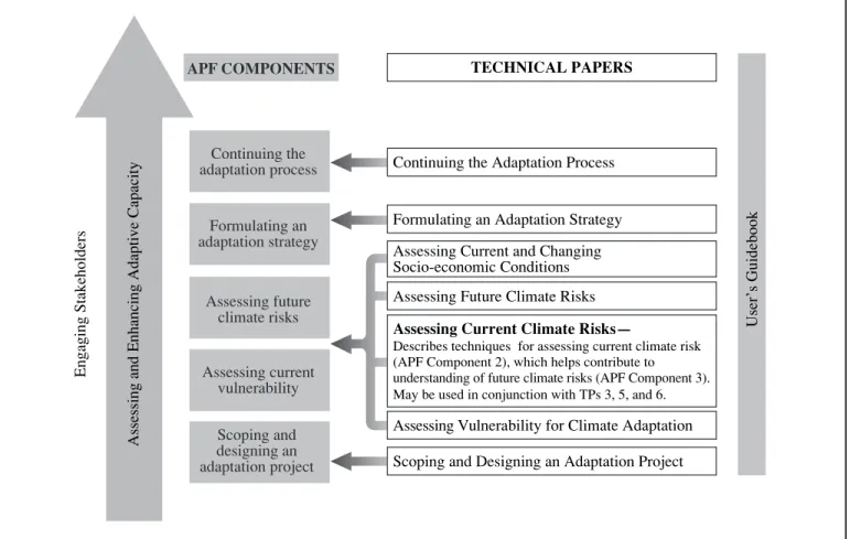
4.2. Relationship with the Adaptation Policy Framework as a whole
This paper is linked directly to the APF Component 2, Assessing Current Vulnerability. Dealing specifically with cur-rent climate impacts and risks, TP4 takes into account natural resource drivers, socio-economic drivers, adaptation
experi-ence and the policy environment, and is thus connected to other TPs in the following way:
TP2: Engaging Stakeholders in the Adaptation Process – Stakeholders are vital in identifying various aspects of the coping range, including the key climatic variables and criteria for risk assessment, including thresholds. TP3: Assessing Vulnerability for Climate Adaptation – This
TP explores methods of assessing current and future vulnerability to climate change including variability. Methods of assessing vulnerability in TP3 can be combined with methods of hazard identification – out-lined in this TP – to assess risk.
TP5: Assessing Future Climate Risks – This TP describes how climate–society relationships may change under climate change and discusses how climatic information can be applied within a variety of risk assessments. TP6: Assessing Current and Changing Socio-Economic
Conditions – This TP can be used to analyse the chang-ing social responses to past and present climate. These techniques can be used to construct a dynamic view of changes in the ability to cope with climate over time. TP7: Assessing and Enhancing Adaptive Capacity – This
TP describes the potential to respond to an anticipated or experienced climate stress. Analysis of the histori-cal ability to cope with climate risks can indicate the adaptive capacity of a particular system.
TP8: Formulating an Adaptation Strategy – This TP looks at specific choices to adapt to risks recognised in this TP and TP5.
4.3. Key concepts
4.3.1. Risk
Risk is a term in everyday use, but is difficult to define in prac-tice due to the complex relationships between its Components. Risk is the combination of the likelihood (probability of occur-rence) and the consequences of an adverse event (e.g., climate hazard)1. In this TP, we describe the major elements of risk such as hazard, probability and vulnerability, though other ter-minology (e.g., exposure) can be used (TP3). These elements of risk can be applied in various ways depending on factors such as the level of uncertainty, whether the focus of an assess-ment is broad or specific and on the direction and emphasis of the approach used. Here, we describe two major approaches to assessing climate risk, a natural hazards-based approach and a vulnerability-based approach. These approaches rely most on whether the starting emphasis is on the biophysical or the socio-economic aspect of climate-related risk. In other words, is the emphasis on the climate hazard or on socio-economic outcomes? These two approaches are complementary and can be developed separately or together.
A hazard is an event with the potential to cause harm. 1Beer and Ziolkwoski, 1995; USPCC RARM, 1997.
Examples of climate hazards are tropical cyclones, droughts, floods, or conditions leading to an outbreak of disease-causing organisms (plant, animal or human). Probabilities can be asso-ciated with the frequency and magnitude of a given hazard, or with the frequency of exceedance of a given socio-economic criterion (e.g., a threshold). Probability can range from being qualitative (using descriptions such as “likely” or “highly con-fident”) to quantified ranges of possible outcomes, to single number probabilities. Vulnerability is broadly defined in TP3. Here, we limit our use of the term vulnerability to refer to cli-mate vulnerability – specifically, the outcomes of clicli-mate haz-ards in terms of cost or any other value-based measure. Specific vulnerabilities (e.g., to drought, flood or storm surge) can also be assessed within the investigation of more broadly based social vulnerability, as described in TP3.
4.3.2. Natural hazards-based approach
The natural hazards-based approach to assessing climate risk begins by characterising the climate hazard(s) and can be writ-ten as:
Risk = Probability of climate hazard x Vulnerability
Hazard is generally fixed at a given level and used to estimate changing vulnerability over space and/or time. For example, a flood of a given height or a storm with a given wind speed may increase in frequency of occurrence over time, increasing the risk faced (assuming that vulnerability remains constant).
4.3.3. Vulnerability-based approach
The vulnerability-based approach begins by characterising vul-nerability to produce criteria by which risk is assessed, e.g., by assessing the likelihood of exceeding a critical threshold. Risk = Probability of exceeding one or more criteria of
vulner-ability2
Fixing the level of vulnerability allows the magnitude and frequency of climate-related hazards contributing to that vulner-ability to be diagnosed. This is the “inverse method” as described in Carter et al. (1994). While commonly used in other disci-plines, this technique has not been widely used for assessing cli-mate change risks. If adaptation occurs, then successively larger and/or more frequent climate hazards can be coped with (e.g., a farming system adapting to drought should be able to manage Continuing the Adaptation Process
Userʼs Guidebook
Assessing Vulnerability for Climate Adaptation Formulating an Adaptation Strategy
Assessing Current Climate Risks—
Describes techniques for assessing current climate risk (APF Component 2), which helps contribute to
understanding of future climate risks (APF Component 3). May be used in conjunction with TPs 3, 5, and 6. Assessing Future Climate Risks
Assessing Current and Changing Socio-economic Conditions
Scoping and Designing an Adaptation Project Scoping and designing an adaptation project Assessing current vulnerability Assessing future climate risks Formulating an adaptation strategy Continuing the adaptation process TECHNICAL PAPERS APF COMPONENTS Asse
ssing and Enhancing Adaptive
Capacity
Engaging St
akeholders
Figure 4-1:Technical Paper 4 supports Components 2 and 3 of the Adaptation Policy Framework
2Other formulations of risk are possible, but most will fall into the above two groups. Here, we have tried to provide a broad framework for assessing risk that will encompass more specific approaches.
more severe droughts before that system becomes vulnerable). Two other methods mentioned in TP1 are the policy-based approach and the adaptive-bcapacity approach:
• Risk assessment techniques can be used in the policy-based approach where:
• a new policy being framed is tested to see whether it is robust under climate change;
• an existing policy is tested to see whether it manages anticipated risk under climate change.
• The adaptive-capacity approach investigates a system to determine whether it can increase the ability to cope with climate change, including variability. This approach will also be informed by a better knowledge of climate risks.
4.3.4. Adaptation, vulnerability and the coping range
Over time, societies have developed an understanding of climate variability in order to manage climate risk. People have learned to modify their behaviour and their environment to reduce the harmful impacts of climate hazards and to take advantage of their local climatic conditions. They have observed biophysical and socio-economic systems responding automatically to cli-mate, and have tried to understand and manage these responses. This social learning is the basis of planned adaptation. Planned adaptationis undertaken by all societies, but the degree of appli-cation and the methods used vary from place to place. In
mod-ern societies, public sector adaptation may rely largely on sci-ence and government policy, and private sector adaptation on market forces, business models and regulation. Traditional soci-eties may rely on narrative traditions, bartering of trade goods and local decision-making. All of these methods can be expressed using a common template.
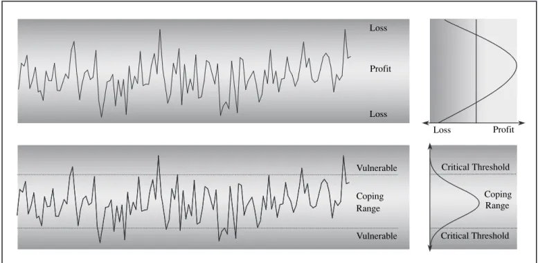
This template has three climate ranges, depending on whether the outcomes are beneficial, negative but tolerable, or harmful. Beneficial and tolerable outcomes form the coping range (Hewitt and Burton, 1971). Beyond the coping range, the dam-ages or losses are no longer tolerable and an identifiable group is said to be vulnerable. This structure is shown in Figure 4-2. A coping range is usually specific to an activity, group and/or sector, though society-wide coping ranges have been proposed (Yohe and Tol, 2002). The coping range provides a template that is particularly suitable for understanding the relationship between climate hazards and society. It can be utilised in risk assessments to provide a means for communication and, in some cases, may provide the basis for analysis.
The climatic stimuli and their responses for a particular locale, activity or social grouping can be used to construct a coping range if sufficient information is available. For example, in an agricultural system, this may include aspects of rainfall variabili-ty, temperature and other important prerequisites for understand-ing crop growth, information about crop yield and prices and knowledge of what constitutes a sustainable level of yield. Analyses can then be used to show which levels of yield are good, marginal, poor and which pose a serious threat. For a water
sys-Profit Loss Loss Coping Range Vulnerable Vulnerable Loss Profit Critical Threshold Critical Threshold Coping Range
Figure 4-2:Simple schematic of a coping range under a stationary climate representing rainfall or temperature and crop yield. Vulnerability is assumed not to change over time. The upper time series and chart shows a relationship between climate and profit and loss. The lower time series and chart shows the same time series divided into a coping range using critical thresholds to separate the coping range from a state of vulnerability.
tem, climate drivers may include accumulated rainfall and evapo-ration, if supply is being addressed, or rainfall intensity and dura-tion, if flooding is being addressed. On a coastline, climate vari-ables contributing to storm surge, tidal regimes and sea level anomalies may be linked to thresholds related to the degree of coastal flooding or property damage. Coping range Components can range from simple “rule of thumb” estimates to accurate rep-resentations of a system based on detailed modelling.
Figure 4-2, upper left, shows a time series of a single variable, e.g., temperature or rainfall, under a stationary climate. If condi-tions get too hot (wet) or cold (dry), then the outcomes become negative. The response curve on the upper right represents the relationship between climate and levels of profit and loss for some measure, e.g., crop yield. Under normal circumstances, outcomes are positive but become negative in response to extremes of climate variability.
Using a response relationship between climate and other dri-vers and specific outcomes, we can select criteria or indicators representing different levels of performance for the purposes of assessing risk (Figure 4-2, lower left). For example, a yield relationship can be divided into good, poor or disastrous seg-ments or coping capacity can be delimited by a critical thresh-old. More complex criteria, perhaps based on vulnerability analysis (TP3, Activities 2 and 3), may represent factors such as the ability to grow next season’s seed supply, grow next year’s food supply, break even economically, or produce suffi-cient surplus to pay for supplementary food and children’s school fees. Note that in Figure 4-2, the critical threshold rep-resenting the ability to cope is held constant, but in the real world is dynamic, responding to internal process in addition to external climatic and non-climatic drivers (Annex A.4.3). By adapting the knowledge of climate–society relationships held within a community, as well as within public and private institu-tions, the project team may be able to develop a relationship link-ing climate to criteria that represent a given level of vulnerabili-ty. For example, a narrative history of past droughts and the responses to those droughts can be matched with rainfall records to construct a fuller picture of climate–society relationships that can then be assessed under conditions where both climate and society may change (TP2, Activity 2; Tarhule and Woo, 1997). Therefore, risk can be assessed by calculating how often the coping range is exceeded under given conditions (Figure 4-2, lower right). The method of assessing risk can range from qual-itative to quantqual-itative. Qualqual-itative methods can be carried out by building or using an existing conceptual model of a specif-ic coping range and assessing risk in terms of qualifiers such as low, medium and high. Quantitative methods will begin to assess the likelihood of exceeding given criteria, such as criti-cal thresholds. Quantitative modelling will allow these rela-tionships to be assessed under changing conditions. When undertaking mathematical modelling using the coping range, it is advisable to modify the mathematical models to suit the con-ceptual models rather than let the structure of the models dom-inate the assessment.
The coping range is a very useful concept because it fits the mental models that most people have concerning risk. People have an intuitive understanding of the situations they face regarding commonly encountered climatic risks – which risks can be coped with, which cannot and what the consequences may be. This understanding can be extended to other less com-monly encountered risks and to never before experienced situ-ations that may occur under climate change. Stakeholders will also have different coping ranges. An assessment may wish to explore those differences in order to gather a common activity-wide coping range for the purposes of assessment, or to explore the differences between coping ranges, e.g., why do certain groups cope better with a situation, and how do we share that capacity with others?
4.4. Guidance on assessing current climate risks
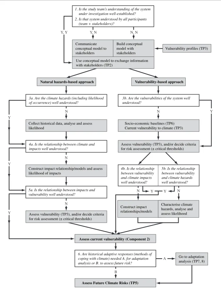
The goal of this section is to guide the user through the process of assessing current climate risks, as outlined in Figure 4-3, rather than provide a tight prescription for how to proceed. There are two major paths one can use, depending on whether the starting point focuses on climate or on vulnerability to cli-mate. For example, a project focusing on the identification of regional climate hazards and how they may alter vulnerability will probably be more suited to a natural hazards-based approach. Approaches focused on the nature of vulnerability or critical thresholds may well start at that point then work back-wards to determine the magnitude and frequency of hazards contributing to that vulnerability. Natural hazards-based approaches are favoured where the probabilities of the climate hazards can be constrained, where the main drivers of impacts are known and where the chain of consequences between haz-ard and outcome is well understood. The vulnerability-based approach will be favoured where: the probability of the hazard is unconstrained, there are many drivers and there are multiple pathways and feedbacks leading to vulnerability. Steps can be carried out in any order to suit the needs of an assessment and can be skipped if they are not considered necessary. Previous information on risks and hazards can also be introduced. The most basic elements needed are a conceptual model of the sys-tem and a basic knowledge of the hazards and vulnerabilities in order to prioritise risk. Both qualitative and quantitative meth-ods can be used to assess risk depending on the quality of infor-mation needed by stakeholders and the data and knowledge available to provide that information.
4.4.1. Building conceptual models
Component 2 of the APF requires an understanding of the important climate–society relationships within the system being investigated. Those relationships are dominated by the climate impacts within the system and the sensitivity of the system response. Climate sensitivityis defined as the degree to which a system is affected, either beneficially or adversely, by climate-related stimuli (IPCC, 2001). Sensitivity affects the magnitude and/or rate of a climate-related perturbation or
1. Is the study team’s understanding of the system under investigation well-established? 2. Is that system understood by all participants (team + stakeholders)?
Vulnerability profiles (TP3)
Use conceptual model to exchange information with stakeholders (TP2) Communicate conceptual model to stakeholders Build conceptual model with stakeholders Vulnerability-based approach
3b. Are the vulnerabilities of the system well understood?
Socio-economic baselines (TP6) Current vulnerability to climate (TP3)
Assess vulnerability (TP3), and/or decide criteria for risk assessment (± critical thresholds)
4b. Is the relationship between vulnerability and climate impacts well understood?
Construct impact relationships/models
Characterise climate hazards, analyse and assess likelihood
5b. Is the relationship between vulnerability and climate hazards well understood?
Assess current vulnerability (Component 2)
6. Are historical adaptive responses (methods of coping with climate) needed A. for adaptation analysis or B. to assess future risk?
Go to adaptation analysis (TP7, 8)
Assess Future Climate Risks (TP5)
3a. Are the climate hazards (including likelihood of occurrence) well understood?
Collect historical data, analyse and assess likelihood
4a. Is the relationship between climate and impacts well understood?
Construct impact relationship/models and assess likelihood of impacts
5a. Is the relationship between impacts and vulnerability well understood?
Assess vulnerability (TP3), and/or decide criteria for risk assessment (± critical thresholds)
Natural hazards-based approach
Y, Y N Y Y N N N Y Y N N B A Y Y Y, N N, N
stress, while vulnerability is the degree to which a system is susceptible to harm from that perturbation or stress (TP3 pre-sents the development of conceptual models for assessing vulnerability).
Climate–society relationships can be identified through stake-holder workshops, or may be well known from previous work. The creation of lists, diagrams, tables, flow charts, pictograms and word pictures will create a body of information that can be further analysed. TP2 describes a number of ways this can be carried out with stakeholders. Establishing conceptual models in the early stages of an assessment can help the different par-ticipants develop a common understanding of the main rela-tionships and can also serve as the basis for scientific model-ling. In this chapter, we utilise the coping range extensively because of its utility as a template for understanding and analysing climate risks, but it is not the only such model that can be used. Other models include decision support systems, causal chains of hazard development, and mapping analysis (e.g., using geographic information systems). A comprehensive list of methods is provided in TP3.
4.4.2. Characterising climate variability, extremes
and hazards
The characterisation of climate variability begins with under-standing the aspects of climate that cause harm, i.e.,the climate hazards. With reference to the coping range, climate hazards are the aspects of climate variability and extremes that have the potential to exceed the ability to cope.
A starting question could be: “Are the climate hazards (affect-ing the system) known and understood?” There are two steps to this: the identification of the relevant climate hazards and their analysis. If the hazards for a system need to be identified, or their impact on the system investigated, the following questions can be addressed:
• Which climate variables and criteria do stakeholders use in managing climate-affected activities?
• Which climate variables most influence the ability to cope (i.e., those linked to climate hazards)?
• Which variables should be used in modelling and sce-nario construction?
These questions can be investigated by ways such as:
• Moving through a comprehensive checklist of climate variables in stakeholder workshops.
• Literature search, expert assessment and information from past projects.
• Exploring climate sensitivity with stakeholders, through interview, survey or focus groups.
• Building conceptual models of a system in a group environment.
Different aspects of climate variability will need to be exam-ined. For example, rainfall can be separated into single events, daily variability and extremes, seasonal and annual totals and variability, and changes on longer (multi-annual and decadal) timescales. Daily extremes are important in urban systems for flash-flooding, inter-annual variability for disease vectors, and seasonal rains for dry-land agriculture. Temperature can be divided into mean, maximum and minimum daily averages, variability and extremes. In each system, people will have a dif-ferent set of variables that they use to manage that system. Even though this management may not be scientific, it may be very sophisticated. Each of these variables involves a different level of skill in terms of climate modelling and has different degrees of predictability under climate change – information that is critical for building climate scenarios.
Hazards are not the same as extreme events, though they are related. Hazards are events and combinations of events with a propensity to cause harm, whereas extreme events are defined through rarity, impact, or a combination of both. Some extreme
Type Description Examples of events Typical method of
characterisation
Simple Individual local weather
vari-ables exceeding critical levels on a continuous scale
Heavy rainfall, high/low temperature, wind speed
Frequency/return period, sequence and/or duration of variable exceeding a critical level
Complex Severe weather associated with
particular climatic phenomena, often requiring a critical combi-nation of variables
Tropical cyclones, droughts, ice storms, ENSO-related events
Frequency/return period, magni-tude, duration of variable(s) exceeding a critical level, severi-ty of impacts
Unique or singular A plausible future climatic state with potentially extreme large-scale or global outcomes
Collapse of major ice sheets, cessation of thermohaline circu-lation, major circulation changes
Probability of occurrence and magnitude of impact
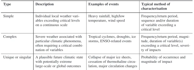
events are defined as such because they occur rarely, such as a one in 100-year flood. Some more common events have extreme impacts, as in hurricanes or tropical cyclones, referred to as extreme events because of the damage they cause, rather than through rarity. Table 4-1 shows a typology of extreme climate events from the Intergovernmental Panel on Climate Change (IPCC) Third Assessment Report (TAR). A number of changes in extremes expected under climate change, and their impacts, are also associated with current extremes (Annex A.4.2). Stress may occur in response to a shock associated with an extreme weather event, or accumulate through a series of events or a prolonged event such as drought. Risk assess-ment requires us to move from characterising extremes to defining hazards.
A climatic hazard is an event, or combination of climatic events, which has potentially harmful outcomes. Depending on the approach taken, hazards can be characterised in two ways: the natural hazards-based approach, where the focus is on the climate itself, and the vulnerability-based approachthat stress-es on the level of harm caused by an impact.
• The natural hazards-based approach is to fix a level of hazard, such as a peak wind speed of 10ms-1, hurri-cane severity, or extreme temperature threshold of 35°C, then to see how that particular hazard affects vulnerability across space or time. Different social groupings will show varying degrees of vulnerability depending on their physical setting and socio-eco-nomic capacity.
• The vulnerability-based approach sets criteria based on the level of harm in the system being assessed then links that to a specific frequency, magnitude and/or combination of climate events. For example, if drought is known to harm a social group, we may choose to look at a given level of stress due to crop failure, and then determine the climatic characteristics that cause those shortages. Or if loss of property due to flooding is the level of vulnerability, then the rain-fall and flood peak contributing to that level of flood-ing may constitute the hazard (and may be due to both climate and catchment conditions caused by land-use change). The level of vulnerability that provides this trigger can be decided jointly by researchers and stakeholders, chosen based on past experience or defined according to policy.
Figure 4-3 provides pathways for both of these approaches.
4.4.3. Impact assessment
Impact assessment under current climate can be used to estab-lish a framework for how a climate hazard acts on society, or can look at vulnerability, then determine which climate hazards are involved. Qualitative methods can stand alone, or can estab-lish the relationships prior to a modelling study.
Qualitative methods
Relationships between climate variables and impacts can be analysed by a number of methods such as ranking in order of importance, identifying critical control points within relation-ships, and quantifying interactions through sensitivity analy-sis (e.g., through workshops, focus groups and question-naires). Often, this knowledge exists in institutions (e.g., agri-cultural extension networks) where important relationships are well known. In such cases, stakeholder workshops may allow the information to be gathered relatively easily. In other situations, several stakeholder workshops may be needed, the first to familiarise stakeholders with the issue of climate change (TP5, Figure 5-2) and to establish areas of shared knowledge and gaps, before investigating the specifics of a particular activity (TP2). Cross-impacts analysis, detailed in Annex A.4.1, can be used to manage the information gathered at such workshops.
The exploration of climate sensitivity with stakeholders is part of “learning by doing”. By listing and discussing the climate variables that are important to them, stakeholders can consider the adaptations they currently use, the important thresholds or criteria they use in management and how those variables might change under climate change (TP2, Activity 3). Scenario builders and impact researchers have the opportunity to ask stakeholders which types of climatic events are important to them, and how they have responded to extreme events in the past (e.g., the relationship between climate events and changes in adaptive capacity, see TP7). This process is very useful if introduced with an overview of climate change and expected impacts. It is also an opportunity to discuss the policy and insti-tutional environment, how non-climatic factors interact with climate in specific activities and issues of sustainable develop-ment (Activity 4, TP3). For example, in Bangladesh, damage from cyclones of the same intensity was US$1,780 million in 1991 and US$125 million in 1994. Reduction in damage was mainly due to setting up institutions after the 1991 cyclone and effective cyclone preparedness in 1994.
Quantitative methods
Quantitative impact assessment involves the formal assessment of climate, impacts and outcomes within a modelling frame-work. There is extensive literature on how to carry out impact assessment that includes IPCC assessment reports, impacts and adaptation assessment guidelines, and works within the indi-vidual disciplines (e.g.,Carter and Parry, 1998; Carter et al., 1994; IPCC-TGCIA, 1999; UNEP, 1998).
In assessing current risk, impact modelling will largely con-centrate on assessing the impacts of extreme events and vari-ability, perhaps undertaking modelling to extend the results based on relatively short records of historical data (e.g., through statistical analysis). Sensitivity modelling in testing changes to variability and investigating extreme event proba-bilities can be of benefit later when climate scenarios are
being constructed. Furthermore, given the difficulty in com-bining various types of climate uncertainty (discussed in TP5), sensitivity modelling of impacts under climate variabil-ity will help identify which uncertainties need to be repre-sented in scenarios.
4.4.4. Risk assessment criteria
As mentioned earlier, risk is a function of the likelihood of a harmful event and its consequences. Likelihood can be attached to the frequency of a hazard and/or to the fre-quency of given criteria being exceeded. All risk assess-ments need to be mindful of which criteria are important: what is to be measured and how are values to be attached to various outcomes?
Each assessment needs to develop its own criteria for the mea-surement of risk. Assessment criteria can be measured as a con-tinuous function or in terms of limits or thresholds. For exam-ple, in farming, crop yields can be divided into good, moderate, poor and devastating yields depending on yield per hectare, per family or in terms of gross economic yield. There may be a minimum level of yield below which hardship becomes intol-erable. This level can become a criterion by which risk is mea-sured. It marks a reference point with known consequences to which probabilities can be attached. More sophisticated assess-ment may utilise different frequencies and combinations of good and bad years.
Levels of criteria that associate climate and impacts are known as impact thresholds, where the threshold marks a change in state. Impact thresholds can be grouped into two main cate-gories:biophysicaland socio-economic.
• Biophysical thresholds mark a physical discontinuity on a spatial or temporal scale. They represent a distinct change in conditions, such as the drying of a wetland, floods, breeding events. Climatic thresholds include frost, snow and monsoon onset. Ecological thresholds include breeding events, local to global extinction or the removal of specific conditions for survival. • Socio-economic thresholds are set by benchmarking a
level of performance. Exceeding a socio-economic threshold results in a change of the legal, managerial or regulatory state, and the economic or cultural behav-iour. Examples of agricultural thresholds include the yield per unit area of a crop in weight, volume or gross income (Jones and Pittock, 1997).
Critical thresholdsare defined as any degree of change that can link the onset of a critical biophysical or socio-economic impact to a particular climatic state (Pittock and Jones, 2000). Critical thresholds can be assessed using vulnerability assess-ment and mark the limit of tolerable harm (Pittock and Jones, 2000; Smit et al., 1999). For any system, a critical threshold is the combination of biophysical and socio-economic factors that marks a transition into vulnerability. The construction of a crit-ical threshold can be used to limit the coping range. If this threshold can be linked with a level of climate hazard, then the likelihood of that threshold being exceeded can be estimated subjectively if the relationship is known qualitatively, or calcu-lated if the relationship is quantifiable.
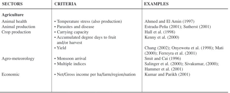
Table 4-2 lists a number of criteria, including thresholds, which have been used in climate risk assessments. They range from the biophysical to the socio-economic, from being universal to context-specific, and from the subjective to the objective. For example, economic write-off for infrastructure is
socio-eco-• Temperature stress (also production) • Parasites and disease
• Carrying capacity
• Accumulated degree days to fruit and/or harvest
• Yield
• Monsoon arrival • Multiple indices
• Net/Gross income per ha/farm/region/nation
Ahmed and El Amin (1997)
Estrada-Peña (2001); Sutherst (2001) Hall et al. (1998)
Kenny et al. (2000)
Chang (2002); Onyewotu et al. (1998); Mati (2000); Ferreyra et al. (2001)
Smit and Cai (1996)
Salinger et al. (2000); Sivakumar, (2000); Hammer et al. (2001)
Kumar and Parikh (2001)
SECTORS CRITERIA EXAMPLES
Agriculture Animal health Animal production Crop production Agro-meteorology Economic
• Vulnerable • Endangered
• Sustainable population levels
• Climate envelope shifts beyond current distribution
• Quantified change in core climatic distribution
• Climatic thresholds affecting distribution • Critical levels of mean browsing intensity • Climatic threshold between eco-geomorphic
systems
• Mass bleaching events on coral reefs • Winter chill – e.g., frequency of occurrence
below daily min. temp. threshold • Cumulative degree days for various
biological thresholds
• Day length/temperature threshold for breeding
• Temperature threshold for coral bleaching
• Salinity
• Flooding and wetlands • Mangroves
• Planning for disasters/hazards • Coastal dynamics
• Critical thresholds for atolls
• Regional assessment/multiple factors • Infrastructure/economics
• Distribution
• Regulated water quality standards for factors such as salinity, dO, nutrients, turbidity. • Regulated and/or legislated annual supply at
system, district at farm level • Water storage stress
• Renewable supply/water stress • Institutional frameworks
• Maintenance or low-flow event frequency and duration
• Change in runoff and streamflow • Flood events
• Palmer drought severity index • Drought exceptional circumstances • Current mean and minimum energy supply
Country/species specific
Villers-Ruiz and Trejo-Vásquez, 1998)
Kienast et al. (1999) Lavee et al. (1998) Hoegh-Guldberg (1999)
Hennessy and Clayton-Greene (1995), Kenny et al. (2000)
Spano et al. (1999) Reading (1998)
Huppert and Stone (1998)
Nicholls et al. (1999) Ewel et al. (1998) Arthurton (1998) Pethick (2001) Dickinson (1999)
Perez et al. (1996); Yim (1996) El Raey (1997)
Somaratne and Dhanapala (1996); Eeley et al. (1999)
Widespread and locally specific. Jones (2000); Bronstert et al. (2000) Lane et al. (1999)
Jaber et al. (1997)
Arnell (1999); Savenije (2000) El-Fadel et al. (2001)
Panagoulia and Dimou (1997) Mkankam Kamga (2001)
Panagoulia and Dimou (1997); Mirza (2002) Palmer (1965)
White and Karssies (1999) Mimikou and Baltas (1997)
SECTORS CRITERIA EXAMPLES
Biodiversity Species or community abundance Species distribution Ecological processes Phenology Coastal zone General Forestry Hydrology Water quality Water supply Streamflow Flooding Drought Hydroelectric power
nomic, context-specific and subjective, based on assumptions used in cost-benefit analysis. Degree-days to harvest for a crop is biophysical, universal and objective, but a threshold based on economic output from that crop will be socio-economic, con-text-specific and probably subjective.
Criteria for risk assessment can be developed using vulnerabil-ity analysis (TP3). Where criteria are context-specific, stake-holders and investigators can jointly formulate criteria that become a common and agreed metric for an assessment (Jones, 2001). These may link a series of criteria ranked according to outcomes (e.g., low to high), or be in the form of thresholds. Critical thresholds can be defined simply, as in the amount of rainfall required to distinguish a severe drought, e.g., <100 mm rainfall over a dry season, or can be complex, such as the accu-mulated deficit in irrigation allocations over a number of sea-sons (Jones and Page, 2001; TP5 Annex A.5.1). Widely applic-able thresholds can be obtained from the literature. Other thresholds may be legal or regulatory (e.g., building safety standards, water quality standards).
There are no hard and fast rules for constructing thresholds – they are flexible tools that mark a change in state that is con-sidered important. For example, stakeholders may link a given deficit of rainfall with drought hardship that leads to regional out migration, or loss of fresh water supply. Although annual and seasonal total rainfall is on a continuous scale, a change in behaviour associated with given amounts may constitute a threshold. Thresholds can vary widely over time and space, so
each assessment has to identify the adequate criteria. This will depend on a trade-off between the level of information avail-able and what criteria are considered important.
4.4.5. Assessing current climate risks
This section demonstrates different methods of assessing risk under current climate. Within the broad framework of assessing risk, it is possible to conduct assessments that range from being qualitative to those that apply numerical techniques. As uncer-tainty decreases, the use of analytic and numerical methods increase, and the capacity to understand the system over chang-ing circumstances increases. The followchang-ing list outlines this development:
1. Understanding the relationships contributing to risk 2. Relating given states with a level of harm (e.g., low,
medium and high risk)
3. Using statistical analysis, regression relationships 4. Using dynamic simulation
5. Using integrated assessment (multiple models or methods) These methods can be used to undertake the following investi-gations:
• Understanding the relationship between climate and society at a given point in time
• Establishing current climate and society relationships • Aggregate epidemic potential
• Climatic envelope/indices of disease vector • Critical density of vector to maintain virus
transmission
• Heat and cold temperature levels and duration • Disease and disaster
• Economic “write off”, e.g., replacement less costly than repair
• Infrastructure condition falling below given standard
• Threshold for overland flow erosion
• Catastrophic collapse and flooding • Loss of ecosystem
Patz et al. (1998)
McMichael (1996); Hales et al. (2002) Jetten and Focks (1997); Martens et al. (1999); Lindblade et al. (2000a & b) McMichael (1996)
Patz and Lindsay (1999); Epstein (2001); Watson and McMichael (2001)
See TP8 for cost-benefit analysis
Tucker and Slingerland (1997)
Richardson and Reynolds (2000) Foster (2001)
SECTORS CRITERIA EXAMPLES
Human Health Vector-borne diseases Thermal stress Multiple Indices Infrastructure Land degradation Erosion Montane systems Glacial lakes
prior to investigating how climate change may affect these relationships (e.g., setting an adaptation baseline) • Developing an understanding of how past adaptations
have affected climate risks
• Assessing how technology, social change and climate are influencing a system, in order to be able to sepa-rate changes due to climate variability from changes due to ongoing adaptation (e.g., Viglizzo et al., 1997) • Assessing how known adaptation strategies can
fur-ther reduce current climate risks
Choice of method
The following examples show that there are a number of ways to assess climate risk. The method applied in Box 4-1 is haz-ard-driven, starting with the frequency and magnitude of extremes and their relationship to property damage and insur-ance claims. The assessment in Box 4-2 deals with famine, and in Box 4-3 with malarial outbreaks. In both cases, they have begun with the impacts causing vulnerability, and then identi-fied the climate hazard driving those impacts. Adaptation in the form of early warning systems has been applied in the first case and recommended in the second. In both cases, socio-econom-ic factors also affect the level of vulnerability. In Box 4-2, high prices and conflict make populations more vulnerable to drought. In Box 4-3, land-use change is exacerbating the cli-mate hazard, specifically high minimum temperatures, increas-ing the survival of malaria vectors. Box 4-4 begins with an impact factor, crop yield, then identifies how deviations in yields are increasing over time; although average yields are increasing, so is vulnerability to bad years.
These differences help to explain why this TP does not offer tight prescriptions for constructing risk relationships in Section 4.4. Likewise, Figure 4-3 is not meant to provide sim-ilarly tight prescriptions. Either the right- or left-hand path, or both, can be taken. Questions can be missed. Perhaps this information already exists or is not needed for a particular assessment. It is also possible to start with impacts in the mid-dle of the diagram and work forward to vulnerability and backwards towards hazards. In that case, techniques from TP3, this paper and TP6 could be utilised.
The natural hazards-based approach has been the traditional approach for assessing climate risks but, where the link between hazards and vulnerability are unclear, or where there are complex relationships between climate and non-climatic drivers, a vulnerability-based approach could be considered. This may involve setting desirable or undesirable criteria in the form of thresholds, then determining how hazards con-tributed to meeting or avoiding those criteria. For example, how achievable are given levels of water yield and quality, and food security, if the criteria for those are set first, then levels of exposure to climate hazards are determined? If the type and magnitude of hazard that may breach a given level of vulnera-bility is known, adaptation can then ensure that even larger hazards are managed.
Examples
Box 4-1 describes the vulnerability of property to wind damage in the south-eastern United States. This assessment takes a nat-ural hazards-based approach (the left-hand path in Figure 4-3), where relationships between effective mean wind speed and property damage have been created and expressed in annual insurance claim and damage ratios. Having created these rela-tionships, it would be possible to set thresholds for exceedance, e.g., the level where an insurance company may decide to charge higher premiums or to withdraw protection altogether. Alternatively, such criteria could be used to increase building-strength regulations in high-risk zones.
Box 4-2 describes a natural hazards-based approach to disaster prevention, where an early warning system is used to reduce the risk of famine accompanying drought and to increase the ability of people to cope with drought. The development of a Famine Early Warning System (FEWS) has increased the cop-ing range of local populations, but incomplete uptake of the system, and the short-term nature of adaptation strategies means that significant risks still exist. This suggests that although the FEWS has increased the coping range to current climate variability, the delivery of its outputs needs to be fine-tuned and more widely disseminated. Continuing shocks are continuing to reduce the coping capacity of populations, requir-ing short-term risk management before considerrequir-ing longer-term adaptation options under climate change. This example is one where the current risks are so high, detailed risk assess-ment of possible future conditions are not required to prioritise adaptation options. In addition to short-term food aid, produc-tive assets and viable livelihoods can only be restored by pro-moting longer-term development strategies and investments aimed at addressing the root causes of vulnerability to drought and food insecurity (FEWS NET, March 19, 2003).
Box 4-3 is an example of a risk assessment that follows the right-hand path of Figure 4-3. The investigation begins with an impact – malarial outbreak in highland East Africa – aiming to identify the hazards leading to those impacts. The major reason for the increase in malarial outbreaks was an increase in warmer micro-climates in villages near cleared swamps. This indicated that land use change is a factor in increasing malaria risk through increasing minimum temperatures. However, the basic climatic hazard was associated with the warmer temper-atures of the El Niño event of 1997/98, which caused a malar-ia epidemic in the region. Lindblade et al. (2000a and b) also identified critical thresholds for Anopheles mosquito density that is associated with minimum temperatures. These densities could be used to develop sampling strategies to contribute to early warning systems. The identified hazards were of climatic (El Niño) and socio-economic (land-use change) origin. Further risk assessment under climate change would need to include both climatic and socio-economic drivers of change. Box 4-4 shows an assessment of current climate risks within a system that is also changing due to non-climatic influences. Changing technology and cropping area have influenced rice production in Indonesia, creating a trend that masks the impacts
Box 4-1: Assessing property damage from extreme winds
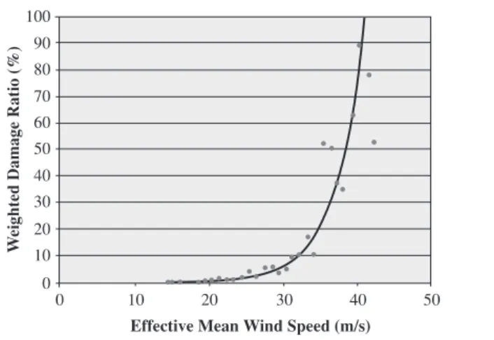
The following example from Huang et al. (2001) assesses property damage from a model of extremes winds. Figures 4-4 and 4-5 show two damage relationships between effective mean wind speed and weighted claim and damage ratios from the southeastern United States. These ratios are the proportion of claims and damages made observed from Hurricanes Andrew and Hugo. One hundred percent of weighted claims or damages indicates that the maximum damage has been reached. Using Monte Carlo modelling of wind fields based on historical hurricane data and the data in Figures 4 and 4-5, Huang et al. (2001) estimated the spatial vulnerability to damage in Florida as expected annual claim and damage ratios for Florida (Figures 4-6 and 4-7).
What critical thresholds or any other criteria measuring vulnerability could be used for the above information? Based on mean wind speed, weighted claims data increase markedly at >20 ms-1; damage ratios increase markedly at >30 ms-1and are a maximum at 41.4 ms-1. Huang et al. (2001) also include information about 50-year return interval wind gusts. Based on levels of property damage, a 2% expected annual damage ratio would see damage occurring to the total value of a build-ing at least once in its 50-year design life. Thresholds could also be set by the insurance industry at levels where damage rates exceed returns. Under climate change, such thresholds may change spatially, or may change in likelihood of exceedance in a single location.
100 90 80 70 60 50 40 30 20 10 0 0 10 20 30 40 50 We
ighted Claim Ratio (%)
Effective Mean Wind Speed (m/s)
100 90 80 70 60 50 40 30 20 10 0 0 10 20 30 40 50 We
ighted Damage Ratio (%)
Effective Mean Wind Speed (m/s) Figure 4-4:Claim ratio vs. effective mean surface
wind speed
Figure 4-5:Damage ratio vs. effective mean surface wind speed N E W S Expected Annual Claim Ratio (%) 0.0 - 5.0 5.0 - 10.0 10.0 - 15.0 15.0 - 20.0 20.0 - 25.0 N E W S Expected Annual Damage Ratio (%) 0 - 0.1 0.1 - 0.4 0.4 - 0.8 0.8 - 1.2 1.2 - 1.6 1.6 - 2.0 2.0 - 3.0 3.0 - 4.0
Figure 4-6:Expected annual claim ratio for each zip code in Florida
Figure 4-7:Expected annual damage ratio for each zip code in Florida
Box 4-2: The use of climate forecasts in adapting to climate extremes in Ethiopia
Introduction
In Ethiopia, famine has long been associated with fluctuations in rainfall. For example, a serious humanitarian disaster occurred during the 1984–5 Ethiopian drought when close to one million people perished. During 2000–1, a more serious drought affected most of Ethiopia. The failure of the 2000 Belg (secondary) rains was more critical compared to the case of 1984. This followed consecutive years of drought in 1998 and 1999, which had killed livestock and over-stretched the coping capacities of local populations. During the year 2000 however, a humanitarian crisis was averted due to a function-ing Famine Early Warnfunction-ing System (FEWS) which had been put in place. However, another drought in 2002 has continued to decrease the ability of populations to cope.
Hazard assessment
The mean rainfall in Ethiopia ranges from about 2000 mm in the southeast to <150 mm in the northeast. There are three seasons:Bega, a dry season (October – January); Belg, a short rain season (February – May) and Kiremt, a long rain sea-son (June – September). Trend analysis showed declining rainfall over the northern half and south-western areas of Ethiopia. A vulnerability assessment showed that a decrease in rainfall over the northern parts of Ethiopia was expected. An investigation with three global climate models also indicated a risk of more frequent droughts under climate change.
Impacts
The major negative impact is on food supply, since Ethiopia is dependent on rain-fed agriculture. Droughts affect the Greater Horn of Africa regularly and the resulting food crisis can easily affect up to twenty million people in Ethiopia alone. Apart from widespread famine, livestock perish and there is potential for armed conflict among communities. Increases in both climate variability and the intensity of drought in Ethiopia are anticipated under climate change.
Adaptation measures
Following the human disaster in 1984, Ethiopia developed a comprehensive Famine Early Warning System, which integrat-ed climate forecasts for Ethiopia with other information such as harvest assessments, vegetation indices and field reports. By 1999, early warning signals showed that a major famine was likely by 2000, due to drought and the border conflict between Ethiopia and Eritrea. As a result, the United States Agency for International Development (USAID) and European Union sig-nificantly increased their food aid commitments. Although there was a significant loss of livestock and livelihoods, a human-itarian disaster was averted. The FEWS played a significant role in sensitising the government and the famine early warning community. This also encouraged small anticipatory actions by affected populations, which improved their coping capacity.
Constraints
In spite of a reasonable FEWS by the year 2000, government and donor decisions were not entirely driven by the FEWS. This meant that the potential maximum coping range could not be achieved in Ethiopia. Often the early warning bulletins did not target the appropriate audience. Secondly, the application of seasonal climate forecasts emphasised short-term responses, increasing the risk of reinforcing short-term strategies at the expense of longer-term adaptations and limiting resilience to increased climate change including variability. By early 2003, yet another drought and high prices had reduced the coping capacity of populations even further, and the FEWS had issued a pre-famine alert for 11.3 million people.
Conclusion
Despite the probabilistic nature of climate forecasts and early warning systems, a well-designed FEWS can improve the resilience and coping capacity of communities to the impacts of climate variability and change. Early warning systems com-bined with good seasonal climate forecasts are cost-effective. Early warning information must be disseminated in a timely way to all stakeholders in formats they can understand or appreciate. However, as the events of 2002–3 show, repeated shocks can reduce coping capacities, requiring even greater intervention by outside agencies.
This text is based on Kenneth Broad and Shardul Agrawala’s report in Science Vol. 289, 8 September 2000; the Initial National Communication of Ethiopia to the UNFCCC and on-line at: http://www.fews.net.
of climate. Despite this upward trend, drought still poses a risk to the majority of farmers in Indonesia. By developing a regres-sion relationship to remove the production-based trend, it is pos-sible to independently analyse the impacts of poor years on pro-duction and therefore, to assess the role of climate on drought risk. It shows that although adaptation is improving crop yields, individual poor years still constitute a risk.
This example has investigated question 4a in Figure 4-3: “Is the relationship between current climate and impacts well under-stood?” A vulnerability analysis of which populations were affected by low yields in bad years and how they were affected would help link climate hazards in terms of the El Niño–Southern Oscillation (ENSO) to vulnerabilities related to crop failure.
4.4.6. Defining the climate risk baseline
An assessment of current climate risks (baseline) is needed for
assessing future risks. Planned adaptation to future climate will be based on current individual, community and institutional behaviours that, in part, have been developed as a response to current climate. Existing adaptation is a response to the net effects of current climate (change, including variability) as expressed by the coping range. Adaptation analogues show that adapting to a future climate is influenced by past behaviour (Glantz, 1996; Parry, 1986; Warrick et al., 1986). This includes both autonomous and planned responses. Adaptation measures need to be consistent with current behaviour and future expec-tations if they are to be accepted by stakeholders. The analysis of behavioural responses to current climate variability also aids in the construction of climate scenarios.
Because the interactions between climate and society are dynamic (see Annex A.4.3 for a detailed explanation, also TP6), a climate-risk baseline needs to be created. This is an initial risk assessment at time = t0, or even t-10, which provides the
refer-Box 4-3: Investigating Malaria risks in highland East Africa
Impacts and vulnerability
As highland regions of Africa historically have been considered free of malaria, recent epidemics in these areas have raised concerns that high elevation malaria transmission may be increasing. Hypotheses about the reasons for this include changes in climate, land use and demographic patterns. The effect of land use change on malaria transmission in the southwestern highlands of Uganda was investigated. Two related studies investigated the role of climate and malaria in highland Uganda and devised critical thresholds of vector density to provide early warnings of new outbreaks (Lindblade et al., 2000a and b).
Hazard assessment
From December 1997 to July 1998, during an epidemic associated with the 1997-8 El Niño, mosquito density, biting rates, sporozoite rates and entomological inoculation rates were compared between eight villages located along natural papyrus swamps and eight villages located along swamps that have been drained and cultivated. Since vegetation changes affect evapotranspiration patterns and thus, local climate, differences in temperature, humidity and saturation deficit between nat-ural and cultivated swamps were also investigated. On average, all malaria indices were higher near cultivated swamps, although differences between cultivated and natural swamps were not statistically significant. However, maximum and min-imum temperatures were significantly higher in communities bordering cultivated swamps. In multivariate analysis using a generalized estimating equation approach to Poisson regression, the average minimum temperature of a village was signif-icantly associated with the number of Anopheles gambiae s.l.per house after adjustment for potential confounding vari-ables. It appears that replacement of natural swamp vegetation with agricultural crops has led to increased temperatures, which may be responsible for elevated malaria transmission risk in cultivated areas.
Critical thresholds linking vector density with malarial outbreaks
Because malaria transmission is unstable and the population has little or no immunity, these highlands are prone to explo-sive outbreaks when densities of Anopheles exceed critical levels and conditions favour transmission. If an incipient epi-demic can be detected early enough, control efforts may reduce morbidity, mortality and transmission. Three methods (direct, minimum sample size and sequential sampling approaches) were used to determine whether the household indoor resting density of Anopheles gambiaes.l, exceeded critical levels associated with epidemic transmission. A density of 0.25 Anopheles mosquitoes per house was associated with epidemic transmission, whereas 0.05 mosquitoes per house was cho-sen as a normal level expected during non-epidemic months. It is feasible, and probably expedient, to include monitoring of Anophelesdensity in highland malaria epidemic early warning systems. Although the local severity of the malaria epi-demic was associated with changing microclimates associated with land use, the positive correlation between average min-imum temperature and household densities of Anopheles mosquitoes shows that warmer seasons associated with El Niño and global warming pose a continuing threat.
ence on which future risks are measured. It is not the same as a climate baseline, which may be 1961–90, or longer. The cli-mate-risk baseline can be tied to a period when both socio-eco-nomic and climate data are available, or to a period when par-ticular infrastructure or policy was put in place. For example, when undertaking a risk assessment of water resources, Jones and Page (2001) used a climate baseline of 1890–1996, but the catchment and water resource management model they used was adjusted at flow rules set in 1996, so the risk became a measure of how the 1996 catchment would have behaved under historical climate. This allows a climate-risk baseline to be established using the full range of historical climate with mod-ern catchment management rules.
4.5. Conclusions
By applying the methods outlined in this TP, the team can assess adaptive responses to past and present climate risks, and gain an understanding of the relationship between current climate risks and adaptive responses. This understanding will provide a basis
for developing adaptive responses to possible future climate risks. The assessment of climate hazards causing present cli-mate vulnerability will also help decide which clicli-mate hazards need to be incorporated into scenario development.
Although an understanding of current climate–society interac-tions is an important starting point for adaptation to future cli-mate, it would be dangerous to assume that new hazards will not arise and that new adaptations may not be needed. In most cases both current and future risk will need to be investigated. If knowledge of current climate risks is already established, then the team may move straight to TPs 5 and 6 to develop an understanding of how climate and socio-economic change may affect future climate risks. However, where current climate vul-nerability is high, then adaptation to those risks will be required to develop sufficient capacity to cope with future risks (e.g., Box 4-3). In this case, basic information about how climate may affect those risks in the future could be sufficient. The assessment of future climate risks is described in TP5. Box 4-4: Calculating climate-driven anomalies in the rice production system of Indonesia
This assessment analysed 20 years of national rice production in Indonesia (BPS, 2000) to determine the impact of annual climate anomalies in a cropping system with an upward trend in yields. In the period 1980–1989, national rice production in Indonesia increased consistently from year to year, the increase slowing after 1989 (Figure 4-8). This increasing trend was due to improvements in crop management technology, variety and expansion of the rice planting area. In order to obtain anomaly data, this trend was removed by applying a regression equation. The steps of analysis are as follows:
1. Develop a regression equation to fit the rice production data
2. Calculate the deviation of observed data from the regression line as anomaly data 3. Separate the production anomalies between normal years and extreme years (Figure 4-8)
4. Evaluate trend of the anomalies between good years and bad years. Good years represent normal climate, while bad years represent extreme dry years due to the ENSO phenomenon.
Figure 4-9 shows that the anomalies for the bad years (squares) became more negative with time while those for good years (diamonds) became more positive over time. This indicates that the production loss due to extreme climate events tends to increase, or that the rice production system is becoming more vulnerable.
25,000,000 30,000,000 35,000,000 40,000,000 45,000,000 50,000,000 55,000,000 79 81 83 85 87 89 91 93 95 97 Year National Rice Pr oduction (ton) -2,000,000 -1,500,000 -1,000,000 -500,000 0 500,000 1,000,000 1,500,000 2,000,000 7 9 81 83 85 87 89 91 93 95 97 Normal El Niño La Niña Non El Niño Drought Year Rice Pr
oduction Anomaly (ton)