A Receiver Oriented MAC Protocol for Wireless Sensor Networks

(1)

A Receiver Oriented MAC Protocol for Wireless Sensor Networks

Luca Campelli, Antonio Capone, Matteo Cesana

Eylem Ekici

Dipartimento di Elettronica e Informazione Department of Electrical and Computer Engineering Politecnico di Milano, Milan, Italy Ohio State University, Columbus OH, United States

{campelli, capone, cesana}@elet.polimi.it [email protected]

Abstract

In this paper we propose SPARE MAC, a TDMA based medium access control (MAC) scheme for data diffusion in Wireless Sensor Networks (WSNs). The rationale behind SPARE MAC is to spare energy through limiting the im-pact of idle listening and traffic overhearing. To this extent, SPARE MAC implements a distributed scheduling solution which assigns to each sensor specific radio resources (i.e., time slots) for reception, summarized as Reception Sched-ules (RS), and spreads the information of the assigned RS to neighboring sensors. A transmitting sensor can conse-quently become active in correspondence of the RS of its intended receiver only.

We analyze the performance of SPARE MAC in terms of throughput, power consumption, and data delivery delay both through analytical models and through detailed sim-ulations. Moreover, we compare the performance of SPARE MAC against SMAC.

1 Introduction

Wireless Sensor Networks (WSNs) are composed of small sized battery operated network devices geared with processing capabilities, wireless communication interfaces, and sensing functionalities. With diminishing cost of com-munication devices, WSNs have emerged as an ideal solu-tions to a large number of applicasolu-tions in both civilian and military scenarios where large network infrastructure is re-quired [1]. Just to mention some of the fields where WSNs can be (or are already) deployed, WSNs can be used for de-tection and tracking, environmental monitoring, industrial process monitoring, and tactical systems. Obviously, tar-get applications determine WSN capabilities and properties. Similarly, applications also determine the choice and design of communication protocols.

For example, if a WSN is used in inaccessible or hostile areas, the network deployment is done in a random man-ner (e.g., dropping sensors from air crafts), which implies that the network should be able to self configure to pro-vide a minimal backbone infrastructure. On the other hand,

WSNs have been proposed also for surveillance and moni-toring applications where the actual position of the sensors can be planned a priori, in contrast to the paradigm of sen-sors regarded as "smart dust" only. WSNs for the support of multimedia traffic [2] and for the monitoring of under-ground soil [3] are good representatives of this latter class of applications. Furthermore, many WSNs feature a con-vergecastcommunication paradigm [4] according to which the information must be delivered to a specific device (clus-ter head, data cen(clus-ter, base station, gateway, etc. . . ).

Regardless of the application, in many cases, battery re-placement is impractical or impossible in WSNs. Therefore, both the design of WSN hardware as well as communica-tion protocols must be done to maximize energy efficiency. At MAC layer, energy efficiency can be achieved through minimization of idle listening, retransmissions, unwanted overhearing, and over-emitting.

In this paper, we propose an energy efficient data centric MAC scheme for data collection in WSNs characterized by low sensor mobility and low-to-moderate traffic. Our solu-tion is well-suited for those target scenarios where the col-lection of sporadic data through multi-hop paths is required and very high energy efficiency is of paramount importance to extend network lifetime. Examples of such applications include environmental monitoring and underground sensing of the soil condition (humidity, density, movements, etc. . . ). Our proposed MAC protocol with Slot Periodic Assign-ment for Reception (SPARE MAC) limits the energy waste due to packet overhearing, packet over-emitting, and idle listening. SPARE MAC is a Time Division Multiple Access (TDMA) based scheme, which implements a distributed scheduling solution that assigns time slots to each sensor for data reception and shares such assignments with neighbor-ing nodes. A transmittneighbor-ing sensor becomes active durneighbor-ing the receiving period of its intended receiver only, limiting afore-mentioned problems of overhearing, over-emitting, and idle listening.

The paper has the following organization: Section 2 de-scribes SPARE MAC operation mode, highlighting the pro-cedures for acquiring and distributing the Reception Sched-1-4244-1455-5/07/$25.00 ©IEEE 2007

(2)

ules (RS). In Section 3, we provide analytical models to evaluate SPARE MAC data delivery delay and power con-sumption. Section 4 is dedicated to the performance eval-uation of SPARE MAC under selected network scenarios. Section 5 comments on the differences between our pro-posal and previously published related works, and Section 6 concludes the paper.

2 SPARE MAC Description

2.1 Rationale

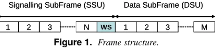
SPARE MAC implements a dynamic Time Division Multiple Access (TDMA) scheme, where all the nodes are time-synchronized. Time synchronization can be achieved via low-power synchronization receivers [5, 6] or through other proposed methods [7, 8, 9]. Furthermore, radio re-sources are organized into periodical frames partitioned into time slots as shown in Figure 1.

To understand the operation of SPARE MAC, we in-troduce the basic concept ofReception Schedule(RS). An RS is defined as a time slot (or group of time slots) dur-ing which a sensor becomes active for receivdur-ing data. In other words, an RS is a portion of the slotted time frame during which a sensor periodically wakes up for data recep-tion. Based on the concept of RS, the basic SPARE MAC philosophy can be summarized with the following two re-quirements:

• Each node is assigned an RS

• Each node knows the RS of all its potential receivers SPARE MAC implements a distributed scheduling so-lution which assigns an RS to each node and spreads the information of the assigned RS to neighboring nodes. The rationale behind SPARE MAC is to spare energy through limiting the impact of unnecessary transmissions, idle lis-tening and traffic overhearing, which are the main causes of energy waste in WSN. In fact, each node running SPARE MAC theoretically becomes active only:

• during the RS of the receiver if it has traffic to send, • during its own RS (limited idle listening),

• when it actually receives the traffic destined to itself only (limited overhearing).

Collisions occur when multiple senders transmit data to the same receiver in the same time slot. SPARE MAC does not prevent collisions from happening, but it reacts to a col-lision event by adopting proper countermeasures.

The RS assignment mechanism outlined above must be supported by a signalling protocol handling both the actual RS reservation and the RS exchange among neighboring

1 2 3 N WS 1 2 3 M

Signalling SubFrame (SSU) Data SubFrame (DSU)

1 2 3 N WS 1 2 3 M

Signalling SubFrame (SSU) Data SubFrame (DSU)

Figure 1. Frame structure.

nodes. In the next sections, we present the implementation details of different components of SPARE MAC. We start off by describing the slotted frame structure (2.2), then we discuss the implementation of the signalling phase, which relies upon the Wake-up Reliable Reservation ALOHA pro-tocol (2.3), and finally we describe the details of the data transfer procedures (2.4).

2.2 Frame Structure and Signalling

Sup-port

SPARE MAC adopts the periodical frame structure shown in Figure 1. Each frame is divided into two sub-frames: aSignalling SUbframe(SSU) and aData SUbframe (DSU) composed ofNandMtime slots, respectively. SSU is used for coordination purposes among neighboring nodes and for the exchange of all topological information needed to perform the scheduling of reception slots. Furthermore, the signalling part also includes aWake-up Slot(WS) slot during which all stations are forced to stay active. Sensors willing to trigger signalling procedures send out a tone in the WS. Details on the usage of the WS and on the sig-nalling procedures are given in Section 2.3. On the other hand, DSU contains data slots which are reserved for data reception. The dimension of the frame depends on the pa-rametersNandM, which in turn depend on the topology of the network and on traffic requirements.

2.3 Wake-up

Reliable

Reservation

ALOHA

The Wake-up Reliable Reservation ALOHA

(WRR-ALOHA) protocol leverages the characteristics of the Re-liable Reservation ALOHAprotocol [13] with the concept of wake-up scheduling. The goals of the WRR-ALOHA protocol are the following:

• to handle the access to the network by new sensors • to assign an RS to each sensor

• to let sensors exchange their RS assignment with one-hop neighbors

The first step for a sensor entering the network (after de-ployment and activation) is to acquire a slot in the SSU. To do so, the new sensor must gather information on the net-work topology and the current radio resource assignment from the already deployed sensors. To this end, the new-comer sends a tone in the wake-up slot, which is received by

(3)

its neighboring nodes. Upon reception of this tone, neigh-boring nodes become active and send out aBroadcast Sig-nalling Packet(BSP) in their own assigned slot during the following SSU. Each BSP contains, besides data and header information, a control field namedFrame Information(FI). The FI is a vector with N entries specifying the status of each of theNslots in the previous SSU preceding the cur-rent transmission, as observed by the transmitting terminal itself. A slot is signalled as BUSY if a BSP has been cor-rectly received from another terminal or transmitted by the terminal itself, otherwise is FREE. In the case of a BUSY slot, the identity of the transmitting terminal is reported.

Consequently, the FIs sent out by each sensor report the information on the activity of neighboring sensors as perceived in the previous SSU. Thus, a sensor receiving the FI from one of its neighbors gets aware of its neigh-bors’neighbors activity. Based on received FIs, the new-comer marks a slot in the SSU, say slot k, either as RE-SERVED or AVAILABLE according to the following:

Rule 1:Slot k is RESERVED, if it is coded as BUSY in at least one of the FIs received; and AVAILABLE, otherwise.

An AVAILABLE slot can be used by the newcomer. Upon accessing an AVAILABLE slot, the newcomer, say sensor j, will recognize in the next SSU the outcome of its access according to the following:

Rule 2The transmission is successful if the accessed slot is coded as "BUSY by sensor j" in all the received FIs; and failed, otherwise.

If the access has been successful, the newcomer stops sending tones in the wake-up slot and goes to sleep. Oth-erwise, the newcomer attempts a new access in another AVAILABLE slot. Furthermore, it keeps sending tones in the wake-up slot until it has successfully acquired a slot in the SSU, thus forcing its neighbors to keep sending out their BSPs.

We emphasize here that the WRR-ALOHA protocol guarantees that any BSP transmission is fully one-hop re-liable, i.e., all one-hop neighbors of the current transmitter correctly receives the transmitted BSP.

The very same BSP transmission procedure is used to assign RS to sensors and to exchange the RS assignments. In fact, each BSP, besides the FI and the transmitter’s ID (see Figure 2), also contains information on the current RS, i.e., indicating the slots selected for reception by the BSP transmitter. Consequently, each sensor receiving BSPs from its neighbors can store its neighbors’ RS, and choose an AVAILABLE RS for itself defined according to the follow-ing:

Rule 3: An AVAILABLE RS must not overlap with any RS of one-hop neighbors.

Rule 3 aims at avoiding those situations where two or more neighboring sensors1 _{cannot communicate because}

they have chosen the very same slots for reception. We ob-serve here that other policies of RS assignment can be im-plemented. For example, RS can be assigned also avoiding overlap with two-hop neighbors RSs.

Both the BSP and RS acquisition procedure outlined above are triggered whenever a new sensor wants to join the network. The RS acquisition and exchange is also triggered whenever any sensor needs to re-schedule its reception pe-riod.

ID 1 N 1 M

Frame Information (FI) Reception Schedule (RS)

ID 1 N 1 M

Frame Information (FI) Reception Schedule (RS)

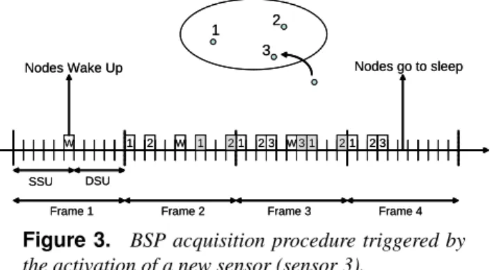
Figure 2. Broadcast Signalling Packet format. Figure 3 shows the case of a new sensor entering the sys-tem (sensor 3). Sensor 3 waits for the next wake-up slot and sends out a tone which activates its neighbors (in frame 1). Neighbors 1 and 2 send out their BSPs in the time slot they have previously acquired (frame 2), further signalling their own RS (shaded slots in the DSU). The information in the BSPs helps the newcomer to choose its own broadcast slot in the SSU, and its own RS in the DSU. As for the broadcast slot, the newcomer randomly picks an AVAILABLE slot in the SSU according toRule 1, say slot 4 in the SSU. As for the RS choice, the newcomer randomly picks an AVAIL-ABLE RS according toRule 3, say slot 1 in the DSU. The new sensor fires its own BSP in the following frame (frame 3), further indicating its own RS (shaded slot in the DSU). In frame 4, the new sensor checks the outcome of its access according toRule 2. Note that the newcomer keeps send-ing power in the WS to force all its neighbors to send their own BSPs until its slot acquisition has been acknowledged. After that, it goes to sleep.

W 1 2 W 1 23 W 1 2 3

Nodes Wake Up Nodes go to sleep

SSU DSU

1 3

2

Frame 1 Frame 2 Frame 3 Frame 4

1 2 31 2

W 1 2 W 1 23 W 1 2 3

Nodes Wake Up Nodes go to sleep

SSU DSU

1 3

2

Frame 1 Frame 2 Frame 3 Frame 4

1 2 31 2

Figure 3. BSP acquisition procedure triggered by the activation of a new sensor (sensor 3).

(4)

2.4 Data Transfer

Once a node has acquired a broadcast signalling slot ac-cording to the procedures explained in the previous section, it can access the radio resources of the DSU. To do so, it maintains a list of its one-hop neighbors with the the cor-responding RS. If the node is a transmitter, i.e., it has data to transfer to a specific one-hop neighbor, it becomes active according to the neighbor’s RS, transmits data and goes to sleep. On the receiver-side, each node wakes up according to its own RS to potentially receive data from its neighbors. We assume here that a node stays active throughout all its RS. Further optimizations in energy conservation are de-ferred to our future work.

Collisions may happen at a receiver when multiple sen-sors transmit on the same RS. To detect such collisions, re-ceivers are required to switch on in the SSU following the DSU and to send out an explicit acknowledgement. A trans-mitter interprets the lack of an acknowledgment as the indi-cation of collision. Collisions are resolved adopting a Col-lision Resolution Algorithm(CRA) based on binary expo-nential backoff. Each colliding station refrains from trans-mitting after a collision for a number of frames,i, computed as:

i=

½

random[1,2k] i f k ≤ 10

210 _otherwise_, (1)

wherekis the number of consecutive collisions experienced by the transmitted packet.

While SPARE MAC conserves energy by avoiding idle listening and overhearing, it does so at the expense of in-creased collision probability. At this point, we emphasize that SPARE MAC is efficient in those situations where data traffic is moderate-to-low on the average, which is the case in many WSN deployments. Under heavy traffic loads, the collision probability, hence the energy consumption, in-creases.

3 Protocol

Analysis

and

Dimensioning

Guidelines

In this section, we present an analytical model for eval-uating the average delay experienced by a packet (Section 3.1) and the average consumed power (3.2) when assuming a single slot RS. Further on, we discuss on the configuration of the SPARE MAC parameters (3.3).

3.1 Delay Analysis

We assume that the total traffic received by a given node is a Poisson process with rate G[packet/frame]. Each trans-mitter sends packets in the first RS of the intended receiver without any initial delay. Within this framework, the total traffic on the channel,G∗, can be written as:

G∗= G 1−Pc, (2) 0 0.4 0.8 1.2 1.6 0 0.5 1 1.5 2 G [kb/s] E [W ] [s ] Ga N=15 M=20 Dtg Gmax

Figure 4.One-hop delay (E[W]) versus offered traf-fic (G) when N=15 and M=20.

wherePc=1−e−G ∗

is the probability for a packet to col-lide. The process of transmission/reception of a packet can be modelled as an M/G/1 queue with the service time dis-tributed according to a random variableX with p.d.f. fX(x)

(wheremXis the mean value andσx2the variance ofX). We

assume thatXis an integer number representing the number of frames for a packet to be correctly received starting from its first transmission attempt.

Thus, the average waiting timeE[W], i.e., the average time an arriving packet has to wait before being received by the intended receiver is given by [10]:

E[W] = ³_ρ_E_[_Z_] 1−ρ +mx− 1 2 ´ ×Tf rame, (3)

where Z is the random variable representing the residual service time as seen by a packet entering the queue given that the server is busy, ρ=mXG, andTf rameis the frame

duration. The term 1/2 is included to account for the aver-age time between the packet arrival and the first RS which is half of a frame duration.

According to the renewal events theory, we can write: E[Z] = mX

2 +

σ2

X

2mX, (4)

By substituting Eq. (4) into Eq. (3), we can express the av-erage waiting time as a function of mean value and variance of the service time, i.e.,mXandσX2. Such quantities depend

on traffic on the channel, which is driven by the specific col-lision resolution algorithms implemented by SPARE MAC. The derivation of closed-form expressions of mX andσX2

for a binary exponential backoff scheme is provided in the Appendix.

Furthermore, we observe that Eq. (3) defines a func-tion which bounds the incoming traffic,G, to the one-hop delay, E[W], in the case each sensor chooses a single-slot RS, E[W] = f(G). In other words, it gives the observed

(5)

delay if all traffic is transmitted using an RS made of a sin-gle slot. This result can be easily used to determine the minimum number of slots in the RS to match a given de-lay constraint. SupposeDtgis the target average delay and

Gmax= f−1(Dtg)the corresponding traffic value. If Ga is

the actual offered traffic, the number of slotsmto be used within the RS to match the constraint on the average delay can be computed as:

m=d Ga

Gmaxe (5)

Consider the following example: Figure 4 shows the single-hop delay predicted by the model versus the chan-nel traffic in the caseN=15 andM=20.DtgandGmaxare

respectively equal to 270 [ms] and 630 [bit/s]. Given the actual incoming traffic,Ga=1.8 [kb/s], the number of slots

mto be used within the RS can be computed using Eq. (5) as:m=d1800

630e=3.

3.2 Energy Analysis

Energy consumption prediction plays an important role in designing solutions for WSNs. Here we present an av-erage power consumption prediction procedure, which de-pends on the process representing the status of the sensors within the frames. The energy status of a sensor within one slot can be transmitting (tx), receiving (rx), sleeping (sl) or idle (id). The total energy consumed by a sensor within a frame is equal to the sum of the energy consumed in each slot of the frame.

Assume that the traffic generated by a given sensor to-wards a specific recipient and the total received traffic are distributed as Poisson point processes with parametersGt

andGrrespectively, measured in[packets/frame]. The

out-going traffic to a receiver,G∗

t, and the incoming traffic,G∗r,

are related to the respective offered traffic through Equation (2), i.e.,

G∗

r =_e−GGr∗r, G

∗

t =_e−GGt∗r. ₍₆₎

If we consider a target sensor, the total energy consumed within a frame depends on whether the sensor will be re-ceiving in a frame and/or transmitting to one or more recip-ients. Under the Poisson assumption for the incoming and outgoing traffic, we can define the following probabilities:

• probability for a sensor to be transmitting towards i recipients in the same DSU:

ptx(i) = ¡_M₋₁ i ¢ (1−e−G∗ t₎i_e−G∗t(M−1−i) (7) with(0 ≤ i ≤ M−1).

• probability for a sensor to be receiving from j∈ {0,1}

transmitters in the same DSU:

prx(0) =e−G∗r prx(1) =1−prx(0) (8)

• the joint probability for a sensor to be transmitting to i recipients and receiving from j transmitters in the same DSU:

phtx(i),rx(j)i = ptx(i)prx(j) (9)

The average consumed energy per frame, Ef, comes from

a weighted average of the energy consumed in transmitting, receiving, idle, and sleeping states. Thus, we can write:

Ef = 1

∑

j=0 M

∑

i=0 phtx(i), rx(j)iE(i,j), (10) whereE(i,j)is the energy consumed in a frame when trans-mitting to i recipients and receiving from j transmitters. Consequently, we can write:

E(i,j) = ierx

s +jetxs + (N−i−j)esls+

+eid

w+ (M−i−j)esld+ietxd +jerxd

(11) whereeyxis the energy consumed in statey(y∈[tx, rx, idle,

sleep]) in a slot of typex(x∈[signalling (s), data (d), wake-up (w)]). Finally, the average consumed power per frame, Pf, can be calculated as:

Pf=_TEf

f rame. (12)

3.3 Frame Dimensioning

Dimensioning a SPARE MAC frame deals with finding optimum values forM andNconsidering the trade-off be-tween capacity, energy consumption, and delivery delay. The value N is strictly bounded by the need of assigning a unique BSP to all sensors in two-hop clusters. Hence,N mainly depends on the topology of the specific WSN. In the network topology shown in Figure 5, the biggest two-hop neighborhood contains S=7 sensors. Therefore, a mini-mumN=7 is required.

Figure 5.Cluster clouds network topology. On the other hand, the valueM is strictly related to the type of application traffic to be delivered. Roughly speak-ing, setting highMdecreases the actual data rate offered at reception and increases the average delivery delay. On the other hand, a large M decreases the average energy con-sumption. Once N is set, the range in whichM can be chosen is given by an interval [Mmin,Mmax], whereMminis

strictly related to the network topology, and can be defined as the dimension of the biggest one-hop neighborhood in

(6)

10 15 20 25 30 35 40 20 40 60 80 100 120 0 5 10 15 20 N M Capacity [kb/s]

Figure 6. Reception capacity versus N and M in the case of single slot RS. Data packets L = 512 bytes. the network. Referring again to Figure 5, the cardinality of the biggest one-hop cluster (the one on the left side) is equal to 5, thusMmin=5. IfMwas equal to 4 two sensors

would be forced to choose the same RS, thus they could not communicate.

On the other hand, Mmax depends on the bandwidth

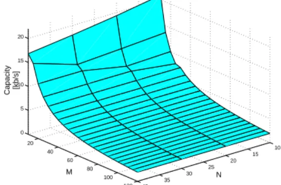
re-quirement of the application. Having in mind the dimen-sioning guidelines ofNandM, the data rate,R, of the chan-nel obtained by assigning a single RS can be calculated as:

R= BRS

NTBSP(N) +MTDP+Tw (13)

whereBRS is the RS dimension (in bits) andTBSP(N),TDP

andTw, are the BSP duration, the RS duration (in seconds),

and the wake up slot duration, respectively. Figure 6 shows the behavior of the reception capacity as a functions of the number of slots in the DSU,M, and the number of slot in the SSU,N.

4 Numerical Results

To test the performance of SPARE MAC, we conducted a simulation analysis in two different WSN topologies shown in Figure 7. In the first topology (Fig. 7.a), each sensor is within the transmission range of all the otherS−1 sensors in the network, thus representing a fully connected network scenario. The second topology (Fig. 7.b) represents the case ofconvergecasttraffic going from leaf sensors to a data sink.

The performance of SPARE MAC in each of these topologies are assessed using three performance metrics: the end-to-end throughput, the end-to-end delivery delay, and the consumed power. All the results presented in this section have been obtained using ns2.29 [12], running 50 simulations for each network configuration and averaging the results. The measured confidence index for all collected statistics is below 5% in 98% of all cases. Table 1 sum-marizes the standard setting of the simulation parameters.

a)

b)

a)

b)

Figure 7. Test topologies: fully connected cluster topology (a), tree topology (b)

Table 1.Standard setting of the simulation parame-ters.

Parameter Value

Simulation Run Length 1000 s

Bandwidth 250 kb/s

Data Slot 560 byte

Signalling Slot 50 byte

Wake-up Slot 9 byte

Packet Length 512 byte

TX Power 24 mW

RX Power 13.5 mW

Idle Power 13.5 mW

Sleep Power 5µW

First, we validate the proposed energy and delay models by comparing them with simulation results in Section 4.1. In Section 4.2, we compare the performances of SPARE MAC and SMAC [14] in theclustertopology, whereas Sec-tion 4.3 studies the performance of SPARE MAC in a multi-hop network scenario where data traffic converges to a sink node.

4.1 Model Validation

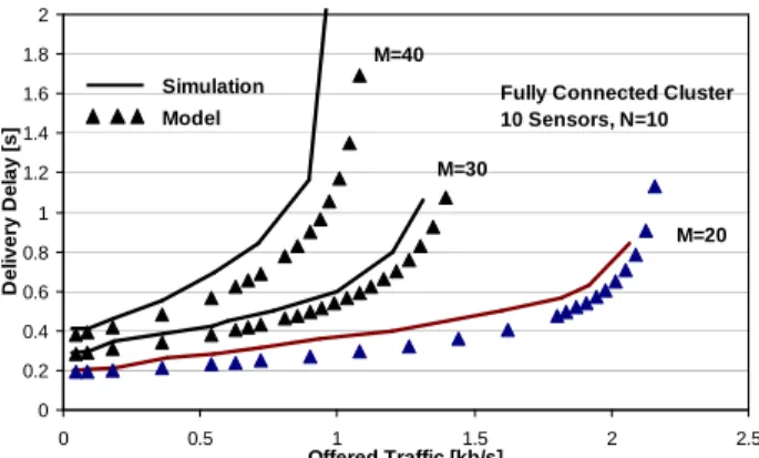
Figure 8 shows the comparison between the average de-lay measured in the simulations and predicted by the model in Section 3.1 in the cluster topology with 10 sensors. As clear from the figure, the delay predicted by the model has the same tendency as the simulated one. The model slightly underestimates the actual delay mainly due to the simplified assumptions on the collision probability.

Regarding the power consumption model, Figure 9 com-pares the simulated values of the consumed power against the one predicted by the model in Section 3.2 in the same one-hop cluster topology as above. Here, the predicted and measured results match closely for the tested traffic loads.

The good match between simulation and analytical model has been observed also for different number of sen-sors within the cluster. The corresponding results are not reported here for the sake of brevity.

4.2 SPARE MAC vs SMAC

We also compared the performance of our proposed SPARE MAC protocol with SMAC, which is one of the

(7)

0 0.2 0.4 0.6 0.8 1 1.2 1.4 1.6 1.8 2 0 0.5 1 1.5 2 2.5 Offered Traffic [kb/s] D e li v e ry D e la y [ s ]

Fully Connected Cluster 10 Sensors, N=10 Simulation Model M=20 M=30 M=40

Figure 8. Average delivery delay versus the offered traffic in the cluster topology with 10 sensors (RS=1). Delay model validation.

0 0.2 0.4 0.6 0.8 1 1.2 1.4 1.6 1.8 2 0 0.5 1 1.5 2 Offered Traffic [kb/s] A v e ra g e C o n s u m e d P o w e r [ m W ] M=40 M=20 Model Simulation

Fully Connected Cluster 10 sensors

N=10

M=30

Figure 9. Average power consumed versus the of-fered traffic in the cluster topology with 10 sensors (RS=1). Power consumption model validation.

most widely adopted MAC protocols. SMAC implements an access scheme based on an evolution of the IEEE 802.11b Distributed Coordination Function to account for energy efficiency. Under SMAC, the radios of the sensors are switched on and off periodically according to specific activity schedules. Sensors exchange their own schedule with other sensors through a synchronization procedure. The main parameters of SMAC are thesync interval, i.e., the interval between two consecutive packets carrying the activity schedules, and theduty cycle, that is, the percent-age of the time each sensors is active with respect to the overall cycle (sleep + active). In the simulations of SMAC, we adopted the same bandwidth and packet lengths reported in Table 1.

Figures 10 and 11 compare the behavior of SPARE MAC and SMAC in the cluster topology by reporting the aver-age consumed power and the averaver-age delivery delay versus the achieved throughput. Under single-hop cluster topol-ogy, every sensor generates Poisson traffic with equal prob-ability to all its neighbors. For each throughput value, we consider those configurations with the highest energy

effi-0 1 2 3 4 5 6 7 0 0.2 0.4 0.6 0.8 1 Throughput [kb/s] A v e ra g e C o n s u m e d P o w e r [m W ] DC=10% DC=20% DC=30% DC=50% M=50 M=40 M=30 M=20 SMAC SPARE MAC Fully Connected Cluster

N=10

Figure 10. Average consumed power versus the achieved throughput in the cluster topology (RS=1,

N=10). Comparison between SMAC and SPARE

MAC. 0 0.2 0.4 0.6 0.8 1 1.2 1.4 1.6 1.8 0 0.2 0.4 0.6 0.8 1 Throughput [kb/s] A v e ra g e D e li v e ry D e la y [ s ] DC=10% DC=20% DC=30% DC=50% M=50 M=40 M=30 M=20 SMAC SPARE MAC

Fully Connected Cluster N=10

Figure 11. Average delivery delay versus the achieved throughput in the cluster topology (RS=1,

N=10). Comparison between SMAC and SPARE

MAC.

ciency, i.e., with the lowest duty cycle in SMAC, and with longest frame (that is, highestM) in SPARE-MAC. From Figure 10, it is clear that SPARE MAC is able to support a given throughput level consuming much less power than SMAC. The power consumption increases linearly with re-spect to the achieved throughput in both cases. However, the SMAC curve is much steeper than the one of SPARE MAC.

As for the delivery delay, SPARE MAC always provides faster delivery with respect to SMAC with a gain ranging from 100 ms at high throughput to 1 s to lower throughput values.

4.3 Convergecast Applications

The network topologies tested so far are uniform with respect to the traffic, where all sensors have the same band-width requirements. However, WSNs devoted to moni-toring and data gathering applications are often deployed and/or organized into hierarchical structures like the one in

(8)

the tree topology of Figure 7. Here, each leaf generates the same traffic amount (Poisson distributed) towards the Sink. Therefore, the total amount of traffic at each level of the tree is different. The traffic bottleneck is represented by the sensors (two in this case) 1 hop away from the sink. To this end, the bandwidth assigned to each sensor must depend on the location of the sensor itself with respect to the traffic and the network topology. As seen in the previous sections, SPARE MAC allows to differentiate the bandwidth assigned in reception to different sensors by increasing/decreasing the number of slots in the correspondent RS.

Intuitively, the dimension of the RS depends on the throughput requirements, the end-to-end delay require-ments of the application, and on the overall energy effi-ciency of the network. The problem of finding the optimal dimensioning can be formulated as the problem of assign-ing the minimum number of slots for reception throughout the network while ensuring a bounded average end-to-end delay and the requested throughput. In a homogeneous tree topology, the problem can be formally stated as follows:

min

_∑

n i=1 miai (14) s.t. n

∑

i=1 Ti ¡Gi mi ¢ ≤Tbound, (15)

wherenis the number of levels in the tree structure,ai is

the number of sensors in each level,mithe number of slots

in the RS at level i, and Ti

¡_G

i

mi

¢

the delay experienced by traffic traversing leveli. Such delay depends on the overall traffic entering leveli,Gi, and the number of slots assigned

to leveli. Since the delay-traffic dependency is non-linear (see Eq. (3) ), so is the constraint (15). It can be shown that the problem can be reduced to an MILP (Mixed Integer Linear Programming) formulation [11]. In the following we provide a simple heuristic to determinemi. Such heuristic

exploits the delay model and the configuration guidelines provided in Section 3.1.

Constraint (15) on the end-to-end delay can be split into several constraints of single-hop delays; namely, if we as-sume to evenly split the delay among different hops, i.e., Ti= Tbound_n , we can easily dimension the single-hop delay,

using the methodology provided in Section 3.1. Given the actual traffic Gleaves generated by the leaves and the

one-hop delay bound,Tbound

n and consequently the corresponding

maximum trafficGmax, the number of slots in the RS,miis

given by Eq. (5), i.e.,mi=d_GG_maxi e, whereGi=Gleaves2i.

In other words, each triplet hGleaves,Tbound,ni induces a scheduling assignment m= [m1,m2, . . .mn] for the tree

topology of Figure 7.b.

Table 2 reports the scheduling assignment for the three levels of sensors in the tree topology of Figure 7.b,mi, in

the case the average end-to-end delay must be bounded at

Table 2.RS dimensions in a three-level tree topology with a end-to-end delay target Dtg=810[ms] when

varying the throughput. N=15, M=20.

Traffic offered by Leaves [kb/s] 0.125 0.25 0.325 0.5 0.625 0.7

m1 2 4 5 7 8 9

RS m2 1 2 3 4 4 5

m3 1 1 2 2 2 3

Dtg=810 [ms], and consequently the per-hop delayTi≤

270 [ms]. Level 1 represents the sink.

Figure 12 reports the end-to-end delay versus the achieved throughput when varying the dimension of the RS according to the dimensioning criteria provided by Table 2. As clear form the figure, the end-to-end delay is kept below the upper bound (810 [ms]) regardless the through-put by adjusting the dimensions of the RS. Obviously, when the throughput increases, the total dimension of the RS, i.e., mtot=∑3k=1mi, increases forcing the sensors to operate with

higher duty cycles; the effect is a higher power consumption throughout the network as represented in Figure 13.

0 0.1 0.2 0.3 0.4 0.5 0.6 0.7 0.8 0.9 1 50 100 150 200 250 300 350 400 450 500 550 600 650 700 750 800

Offered Traffic at leaves [b/s]

E n d -T o -E n d D e la y [ s ] m1=4 m2=2 m3=1 m1=2 m2=1 m3=1 m1=5 m2=3 m3=2 m1=7 m2=4 m3=2 m1=8 m2=4 m3=2 m1=9 m2=5 m3=3 Tree Topology SPARE MAC (N=15, M=20) SMAC (DC=50% )

Figure 12. Average end-to-end delivery delay ver-sus the achieved throughput at the sink in the tree topology. 0 1 2 3 4 5 6 7 8 9 50 100 150 200 250 300 350 400 450 500 550 600 650 700 750 800

Offered Traffic at leaves [b/s]

A v e ra g e C o n s u m e d P o w e r [m W ] m1=2 m2=1 m3=1 m1=4 m2=2 m3=1 m1=5 m2=3 m3=2 m1=7 m2=4 m3=2 m1=8 m2=4 m3=2 Tree Topology SPARE MAC (N=15, M=20) SMAC (DC=50% ) m1=9 m2=5 m3=3

Figure 13. Average power consumption versus the achieved throughput at the sink in thetreetopology.

(9)

The two figures report also the corresponding curves ob-tained under SMAC with adaptive listening, when bound-ing the sbound-ingle-hop average delivery delay at the very same value as above. We observe here that SMAC allows to de-fine just one value for the Duty Cycle (DC) throughout the network, thus the duty cycle of all the sensors depends on the traffic at the sink only2_{(DC=50% in the case of the}

fig-ure). On the other hand, under SPARE MAC, the activity of each sensor is optimized on the local traffic. As clear from Figure 12, SMAC provides lower end-to-end delay at low-moderate traffic, but, on the other hand, it is forced to consume much more power than SPARE MAC (Figure 13).

5 Related Works

In the following we compare qualitatively SPARE MAC against the most common MAC solutions for WSNs. This analysis is not exhaustive since the number of MAC schemes for WSNs proposed in the literature is very large, but it rather aims at highlighting the novel points of SPARE MAC and those network scenarios where it can help.

MAC schemes for WSNs can be categorized as con-tention based and concon-tention free protocols. Concon-tention based schemes resort to some type of random access mech-anism (ALOHA, CSMA, etc. . . ), allowing potential colli-sions on packet transmission to happen, and trying to re-cover from these collisions through proper repetition tech-niques. The SMAC protocol [14], whose performance we compared against SPARE MAC, belongs to this category. The strategy adopted by SMAC follows the one proposed in PAMAS [15], with the difference that, while PAMAS requires an extra radio interface devoted to transmit con-trol information, SMAC uses in-band signalling. SMAC lets the sensors exchange their activity schedules to mini-mize energy consumption due to overhearing and idle lis-tening. Collisions are avoided and resolved through classi-cal CSMA-CA schemes. Variants to SMAC have been pro-posed to let the activity cycle duration be adapted to traffic conditions [16].

Luet al.propose the DMAC protocol [17] for data gath-ering in tree based network topologies. Similarly to SMAC, DMAC adopts periodic sleep-activity cycles with a CSMA-CA approach, but it further introduces the concept of ac-tivity cycles scheduling in order to reduce the latency of transmissions. In other words, sensors know where they are positioned on the tree topology and organize their duty cycle so that the transmission time of sensors belonging to tree level i corresponds to the reception period of sensors of level i-1. In this sense, DMAC shares with SPARE MAC the concept of coordination between sender and receiver, how-ever, the DMAC is contention based and is mainly focused on latency reduction, rather than energy efficiency.

2_{over-dimensioning the duty cycles of leaf sensors}

On the other side, collision free protocols often rely upon dynamic TDMA slotted structures, assume slot synchro-nization among sensors and implements some kind of slot scheduling to assign radio resources to sensors. Valuable examples of TDMA based access schemes are protocols NAMA [19] and TRAMA [18], which share the same de-sign approach. In fact, they both implement a de-signalling phase among two-hop neighbors to eliminate hidden-node collisions and schedule collision-free transmission. How-ever, NAMA does not address energy efficiency, whilst TRAMA lets the nodes go to sleep if they are not en-gaged in transmissions/receptions. Different from SPARE MAC, both TRAMA and NAMA schedule transmission at the sender side, i.e., the sender distributes the information on the radio resource it is going to use. Further on, the schedule distribution procedure in TRAMA and NAMA is implemented with a contention based approach, which can lead to potential collisions on scheduling packets. On the other side, the reception schedule distribution in SPARE MAC exploits a fully reliable collision free broadcast chan-nel.

W MAC [20] is a particular type of TDMA-based MAC protocol which adopts wake-up slots. Each sensor is assigned a couple of slots within a time frame: a wake-up slot where the sensor is actually receiving and a data slot. Whenever a sensors has data to deliver to an in-tended receiver it fires a control packet in the wake-up slot of the intended receiver signalling its own ID. The intended receiver will then switch on again in the next frame in cor-respondence of the data slot of the transmitter. Different from SPARE MAC, TDMA-W MAC assigns data slots to transmitters. On the other side, SPARE MAC implements a receiver-oriented slot assignment and the wake-up slot is devoted to trigger the signalling phase for the distribution of the reception schedules.

6 Concluding Remarks

In this paper we proposed SPARE MAC, an energy effi-cient data centric MAC scheme for data collection in WSNs. SPARE MAC belongs to the category of TDMA based schemes but, different from other TDMA based approaches, the scheduling algorithm is receiver oriented. In fact, un-der SPARE MAC, each sensor is assigned radio resources for data reception and exchanges such assignment with its neighbors. Transmitting sensors can consequently become active in the receiving period of their intended receivers only, limiting overhearing, unnecessary transmissions, and idle listening. Further on, the SPARE MAC provides a reli-able one hop broadcast channel which can be used both for signalling purpose and for the support of broadcast oriented traffic (routing updates, reconfiguration messages, etc. . . ).

We have proposed analytical models for SPARE MAC, validated against simulation results in terms of data deliv-ery delay and energy efficiency. We have tested through

(10)

simulation SPARE MAC performance in terms of achieved throughput, energy efficiency and data delivery delay in one-hop cluster topologies with uniformly distributed traf-fic, and in tree-like topologies for convergecast applications. We have shown that SPARE MAC outperforms SMAC in all tested scenarios.

References

[1] I. F. Akyildiz, W. Su, Y. Sankarasubramaniam and E. Cayirci, A Survey on Sensor Networks,IEEE Communications Maga-zine, vol. 40, no. 8, August 2002, page(s): 102–116.

[2] I. F. Akyildiz, T. Melodia and K. R. Chowdhury, A Survey on Wireless Multimedia Sensor Networks, Computer Networks Journal (Elsevier), vol. 51, no. 4, March 2007, page(s): 921– 960.

[3] I. F. Akyildiz, E. Stuntebeck, Wireless Underground Sensor Networks: Research Challenges, Ad Hoc Networks Journal, vol. 4, July 2006, page(s): 669–686.

[4] I. Demirkol, C. Ersoy, F. Alagoz, MAC Protocols for Wireless Sensor Networks: A Survey,IEEE Communication Magazine, vol. 44, no. 4, April 2006, page(s): 115–121.

[5] A. Rowe, R. Mangharam, R. Rajkumar, RT-Link: A Time-Synchronized Link Protocol for Energy Constrained Multi-Hop Wireless Networks,Proc. of IEEE SECON 2006, page(s): 402–411.

[6] R. Mangharam, A. Rowe, R. Rajkumar, FireFly: A Time-synchronized Scalable Real-time Sensor Network Platform, Proc. of IEEE SECON 2006(poster).

[7] J. Elson, D. Estrin, Time Synchronization for Wireless Sensor Networks,Proc. of IEEE IPDPS 2001, page(s): 1965–1970. [8] I. Rhee, A. Warrier, M. Aia, J. Min, ZMAC: a Hybrid MAC

for Wireless Sensor Networks, Proc. of ACM SenSys 2005, page(s): 90–101.

[9] S. Ganeriwal, R. Kumar, M. Srivastava, Timing-sync proto-col for sensor networks,Proc. of ACM SenSys 2003, page(s): 138–149.

[10] L. Kleinrock,Queuing Systems, Volume I: Theory, Wiley In-terscience, 1975.

[11] L. Campelli, A. Capone, M. Cesana, A MAC Solution for Wireless Sensor Networks based on Slot Periodic Assignment for Reception, Politecnico di Milano, Department of Electron-ics and Information, Technical Report 2007.38, March 2007. [12] Network Simulator 2, website:http://www.isi.edu/

nsnam/ns/.

[13] F. Borgonovo, A. Capone, M. Cesana and L. Fratta, ADHOC MAC: new MAC architecture for ad hoc networks provid-ing efficient and reliable point-to-point and broadcast services, ACM Wireless Networks, vol.10, no. 4, page(s): 359–366, July 2004.

[14] W. Ye, J. Heidemann and D. Estrin, Medium Access Control with Coordinated, Adaptive Sleeping for Wireless Sensor Net-works,ACM/IEEE Transaction on Networking, vol. 12, no. 3, page(s): 493–506, June 2004.

[15] S. Singh and C. S. Raghavendra, PAMAS: Power Aware multi-access protocol with signalling for ad hoc networks, ACM Computer Communication Review, vol. 28, no. 3, page(s): 5–26, July 1998.

[16] T. van Dam , K. Langendoen, An adaptive energy-efficient MAC protocol for wireless sensor networks, Proc. of ACM SenSys 2003, page(s): 171–180.

[17] S. Bandyopadhyay and E. Coyle, An Energy Efficient Hier-archical Clustering Algorithm for Wireless Sensor Networks, Proc. of INFOCOM 2003, vol. 3, page(s): 1713–1723. [18] V. Rajendran, K. Obraczka, J. J. Garcia-Luna-Aceves,

Energy-efficient, collision-free medium access control for wireless sensor networks,ACM Wireless Networks, Feb. 2006, vol. 12, no. 1, page(s): 63–78.

[19] L. Bao, J. J. Garcia-Luna-Aceves, A New Approach to chan-nel access scheduling for ad hoc networks, Proc. of ACM MOOBICOM 2001, page(s): 210–221.

[20] Z. Chen, A. Khokhar, Self organization and energy efficient TDMA MAC protocol by wake up for wireless sensor net-works,Proc. of IEEE SECON 2004, page(s): 335–341.

Appendix: Service Time Mean Value and

Vari-ance

Under the assumptions of constant collision probability, pc, independent on the actual backoff stage,mX can be

ex-pressed as: mX=1−pc+ ∞

∑

i=1 pi_c(1−pc)[mX(i)+1], (16) wheremX(i) is the mean value of the integer random vari-able representing the service time at backoff stagei. Such variable is uniformly distributed in the interval[1,2i_]_{, thus}

we can write: mX(i)= i