Maximum Likelihood Estimation and Lagrange Multiplier Tests for Panel Seemingly Unrelated Regressions with Spatial Lag and Spatial Errors: An Application to Hedonic Housing Prices in Paris

DISCUSSION PAPER SERIES

Forschungsinstitut zur Zukunft der Arbeit Institute for the Study

Maximum Likelihood Estimation and Lagrange

Multiplier Tests for Panel Seemingly Unrelated

Regressions with Spatial Lag and Spatial Errors:

An Application to Hedonic Housing Prices in Paris

September 2010 Badi H. Baltagi Georges Bresson

Maximum Likelihood Estimation and

Lagrange Multiplier Tests for Panel

Seemingly Unrelated Regressions with

Spatial Lag and Spatial Errors:

An Application to Hedonic Housing

Prices in Paris

Badi H. Baltagi

Syracuse University and IZA

Georges Bresson

ERMES (CNRS), Université Panthéon-Assas Paris II

Discussion Paper No. 5227 September 2010 IZA P.O. Box 7240 53072 Bonn Germany Phone: +49-228-3894-0 Fax: +49-228-3894-180 E-mail: [email protected]

Any opinions expressed here are those of the author(s) and not those of IZA. Research published in this series may include views on policy, but the institute itself takes no institutional policy positions. The Institute for the Study of Labor (IZA) in Bonn is a local and virtual international research center and a place of communication between science, politics and business. IZA is an independent nonprofit organization supported by Deutsche Post Foundation. The center is associated with the University of Bonn and offers a stimulating research environment through its international network, workshops and conferences, data service, project support, research visits and doctoral program. IZA engages in (i) original and internationally competitive research in all fields of labor economics, (ii) development of policy concepts, and (iii) dissemination of research results and concepts to the interested public. IZA Discussion Papers often represent preliminary work and are circulated to encourage discussion.

IZA Discussion Paper No. 5227 September 2010

ABSTRACT

Maximum Likelihood Estimation and Lagrange Multiplier

Tests for Panel Seemingly Unrelated Regressions with

Spatial Lag and Spatial Errors:

An Application to Hedonic Housing Prices in Paris

This paper proposes maximum likelihood estimators for panel seemingly unrelated regressions with both spatial lag and spatial error components. We study the general case where spatial effects are incorporated via spatial errors terms and via a spatial lag dependent variable and where the heterogeneity in the panel is incorporated via an error component specification. We generalize the approach of Wang and Kockelman (2007) and propose joint and conditional Lagrange Multiplier tests for spatial autocorrelation and random effects for this spatial SUR panel model. The small sample performance of the proposed estimators and tests are examined using Monte Carlo experiments. An empirical application to hedonic housing prices in Paris illustrates these methods. The proposed specification uses a system of three SUR equations corresponding to three types of flats within 80 districts of Paris over the period 1990-2003. We test for spatial effects and heterogeneity and find reasonable estimates of the shadow prices for housing characteristics.

JEL Classification: C31, C33, R21

Keywords: hedonic housing prices, Lagrange multiplier tests, maximum likelihood, panel spatial dependence, spatial lag, spatial error, SUR

Corresponding author: Badi H. Baltagi

Department of Economics and Center for Policy Research 426 Eggers Hall Syracuse University Syracuse, NY 13244-1020 USA E-mail: [email protected] *

We would like to thank Stuart Rosenthal, Dan Black and anonymous referees for their helpful comments and suggestions. Also, numerous colleagues and conference participants at the Latin American Meeting of the Econometric Society, Buenos Aires, October 1-3, 2009, the First French Econometrics Conference, Toulouse School of Economics, December, 14-15, 2009 and the 16th International Conference on Panel Data, Amsterdam, July 2-4, 2010. Many thanks to Annick Vignes

1

Introduction

Zellner’s (1962) pioneering paper considered the estimation and testing of seemingly unrelated regressions (SUR) with correlated error terms. SUR has been applied in many research areas in economics and other fields, see Srivastava and Giles (1987) and Fiebig (2001) for excellent surveys. It is by now clear that SUR achieves gains in efficiency by estimating a set of equations simultaneously rather than estimating each equation separately. Common factors affecting these equations allow such gains in efficiency and has been demonstrated in economics, for e.g., in studying demand systems and translog cost functions, to mention a few important applications.

Avery (1977) and Baltagi (1980) extended the SUR model to panel data models with error components. This extension allows one to take advantage of panel data which pools regions, counties, countries, neighborhoods over time. Besides the larger variation in the data across these regions, one is able to control for unobserved heterogeneity across these units of observation.

Anselin (1988) extended the SUR model to allow for spatial correlation in the data. This extension allows one to take advantage of spillover effects across regions. Here, we focus on combining the spatial and panel aspects of the data in a SUR context. In fact, Anselin (1988) and Elhorst (2003) among others provided maximum likelihood (ML) methods that combine panel data with spatial analysis, while Kapoor, Kelejian and Prucha (2007) provided a generalized moments estimators (GM) approach for estimating a spatial random effects panel model with SAR disturbances. Fingleton (2008a) extended the GM approach of Kapoor, Kelejian and Prucha to allow for spatial moving average disturbances, see Anselin, Le Gallo and Jayet (2008) for a recent survey.

This paper follows Wang and Kockelman (2007) who applied ML methods to a SUR model with spatial effects incorporatedvia autocorrelation in the spatial error terms and heterogeneity in the panel incorporatedvia random-effects. However, this paper extends the ML approach developed by Wang and Kockelman (2007) to the general case where spatial effects are incorpo-rated via spatial error terms and via a spatial lag dependent variable and where the heterogeneity in the panel is incorporated via an error component specification.

We propose joint and conditional Lagrange Multiplier tests for spatial autocorrelation and random effects for this spatial SUR panel model. The small sample performance of the proposed estimators and tests are examined

using Monte Carlo experiments. We show that ignoring these spatial effects and/or heterogeneity can lead to misleading inference.

An empirical application to hedonic housing prices in Paris illustrates these methods. The proposed specification uses a system of three SUR equa-tions corresponding to three types of flats within 80 districts of Paris over the period 1990-2003.1_{. One of the main contributions of the paper is that it}

pays special attention to the heterogeneity and spatial variation in housing prices across districts and it tests for their existence.2 We find significant spatial effects and heterogeneity across the Paris districts, and we show that ML methods that incorporate these effects lead to reasonable estimates of the shadow prices of housing attributes.

Section 2 sets up the panel SUR model with spatial lag and spatial error components. In section 3, we present the ML estimation under normality of the disturbances. Section 4 considers the problem of jointly testing for random effects as well as spatial correlation in the context of this spatial SUR panel model. This extends earlier work on testing in spatial panel models by Baltagi et al. (2007) from the single equation case to the SUR case. Section 5 performs Monte Carlo experiments which compare the small sample properties of the proposed ML estimators and LM tests. Section 6 provides an empirical application of these methods to the problem of estimating hedonic housing prices in Paris, while section 7 concludes. We recognize that there is a large literature on hedonic housing and that our application is only meant to illustrate our spatial panel ML methods and the the asscociated LM test statistics.

1_{Hedonic measures have a strong theoretical grounding and use regression techniques}

to control for compositional and quality change (see, for example, Arguea and Hsiao (1993), Can (1992), Dubin (1992), Dubin et al. (1999), Griliches (1971), Halvorsen and Pollakowski (1981) and Rosen (1974) to mention a few).

2_{For spatial effects in real estate (see Fingleton (2008b), Glaeser (2008), and Helpman}

(1998) to mention a few). For spatial econometric methods (see Anselin (1988), Anselin and Bera (1998), Anselin et al. (2008), Baltagi (2010), Baltagi et al. (2007), and Elhorst (2003, 2010) to mention a few).

2

The panel SUR with spatial lag and spatial

error components

We consider a spatial system of equations model viewed as an extension of the single equation spatial model introduced by Cliff and Ord (1973, 1981). In particular, we specify a system of spatially interrelated panel equations corresponding to N cross sectional units over T time periods. The spatial SUR model for panel data is composed ofM equations (each potentially hav-ing a different set of explanatory variables) forN regions which are observed over T time periods. Consider the set of M equations:

yjt = γjW yjt+Xjtβj+εjt , j = 1, ..., M, t= 1, ..., T (1)

= γjyjt+Xjtβj +εjt

where yjt is a (N×1) vector,W is an(N ×N)spatial weights matrix3,Xjt

is a (N _×kj) matrix of exogenous variables, βj is a (kj ×1) vector of

para-meters and εjt is a (N ×1) vector of disturbances. The vector yjt(=W yjt)

is typically referred to as the spatial lag of yjt. In addition to allowing for

general spatial lags in the endogenous variables, we also allow for spatial autocorrelation in the disturbances. In particular, we assume that the dis-turbances are generated either by a spatially autoregressive (SAR) process or a spatially moving average (SMA) process:

εjt =

½

λjWεjt+ujt for SAR

λjW ujt+ujt for SMA

(2) andujt is an error component:

ujt =µj+vjt (3)

When we pool theT time periods, we get: yj =γj(IT ⊗W)yj+Xjβj +εj , εj =

½

λj(IT ⊗W)εj +uj for SAR

λj(IT ⊗W)uj +uj for SMA

(4)

3_{For ease of presentation, we are assuming that the system involves only one weight}

matrix. This also seems to be the typical specification in applied work. Our results can be

generalized in a straight forward way to the case in which the weight matrix varies across equations.

with uj = (ιT ⊗IN)µj+vj (5) where µj = ¡ µj1, ...., µjN ¢0 , vj = (vj11, ..., vjN1, ..., vj1T, ..., vjN T)0 and ιT is a

(T _×1)vector of ones, see Anselin, Le Gallo and Jayet (2008). So: y = (Γ_⊗IT ⊗W)y+Xβ+ε , ε= ½ (Λ_⊗IT ⊗W)ε+u for SAR (Λ_⊗IT ⊗W)u+u for SMA (6) where Γ=diagM j=1 © γ_jª andΛ=diagM j=1{λj}.Then, Ay=Xβ+ε ,Bε =u (7) with    A = IN T M−(Γ⊗IT ⊗W) B = ½ IN T M −(Λ⊗IT ⊗W) for SAR [IN T M+ (Λ⊗IT ⊗W)]−1 for SMA (8) or A =    IT ⊗A1 . .. IT ⊗AM   , B =    IT ⊗B1 . .. IT ⊗BM    (9) with Aj =IN −γjW ,Bj = ½ IN −λjW =Hj for SAR (IN +λjW)− 1 =L−_j1 for SMA (10) The variance-covariance matrix of ε is given by:

Ωε =B−1Ωu(B0)−

1

(11) where Ωu is the variance-covariance matrix of the error component term, see

Baltagi (1980): Ωu = [Ωjl] with Ωjl=σµjl(JT ⊗IN) +σvjlIN T (12) = Σu⊗IN =Ωµ⊗JT ⊗IN +Ωv⊗IT ⊗IN = ¡TΩµ+Ωv ¢ ⊗JT ⊗IN +Ωv⊗ET ⊗IN

with JT =JT/T , ET =

¡

IT −JT

¢

andJT is a(T ×T) matrix of ones.

Ωµ =      σ2 µ1 σµ12 · · · σµ1M σµ₂₁ σ2µ2 · · · σµ2M .. . ... . .. ... σµM1 σµM2 · · · σ 2 µM     andΩv =      σ2 v1 σv12 · · · σv1M σv21 σ 2 v2 · · · σv2M .. . ... . .. ... σvM1 σvM2 · · · σ 2 vM     . Based on a joint standard normal distribution for the error term ν =

Ω−u1/2B(Ay−Xβ), the log-likelihood function for the joint vector of

obser-vations y is proportional to: ` ∝₋1 2ln|Ωu|+ ln|B|+ ln|A|− 1 2ν 0_{ν (13)} with ν0ν = (Ay₋Xβ)0B0Ω−_u1B(Ay₋Xβ) (14) = (Ay₋Xβ)0Ω−_ε1(Ay₋Xβ) = ε0Ω−_ε1ε

3

Maximum Likelihood Estimation

`∝    −N2 ln|Σu|+T M P j=1 ln_|Bj|+T M P j=1 ln_|Aj| −12(Ay−Xβ) 0_B0_(Σ−1 u ⊗IN)B(Ay−Xβ) (15)

Using the results in Baltagi (1980) and Magnus (1982),

( |Σu|= ¯ ¯TΩµ+Ωv ¯ ¯_|Ωv| T−1 Σ−1 u = ¡ TΩµ+Ωv ¢−1 ⊗JT +Ω−v1⊗ET (16) we can express the log-likelihood function as follows:

` ∝ ₋N 2 ln ¯ ¯TΩµ+Ωv ¯ ¯₋N(T −1) 2 ln|Ωv|+T M X j=1 ln_|Bj|+T M X j=1 ln_|Aj| −1 2(BAy−BXβ) 0³¡_TΩ µ +Ωv ¢−1 ⊗JT ⊗IN ´ (BAy₋BXβ) (17) −1 2(BAy−BXβ) 0¡_Ω−1 v ⊗ET ⊗IN ¢ (BAy₋BXβ)

Generalizing the Wang and Kockelman (2007) approach, the model can be estimated using a three-step method: First, β can be estimated using gen-eralized least squares (GLS), conditional on Ωµ, Ωv, γ = (γ1, ...,γM)0 , and

λ= (λ1, ...,λM)0.Then Ωµ andΩv can be estimated conditional onβ,γ and

λ. These first two steps are iterated until the optimal Ωµ, Ωv, and β are

found (conditional onγ andλ). The third step is to substitute the estimated

Ωµ,Ωv, andβ and to maximize the concentrated log-likelihood function over

γ andλ. The estimatedγ andλthen re-enter the estimation of Ωµ,Ωv, and

β. This procedure is iterated until convergence.

The estimation method proposed can be performed using the following steps:

3.1

Step 1: Estimate

β

conditional on

Ω

,

Ω

,

γ

and

λ

Note that JT ⊗IN denotes an average of the(BAy−BXβ)values over time

for each equation, and ET ⊗IN denotes each observation’s deviation from

these averages. If one lets P0_{P =} ¡_TΩ

µ+Ωv

¢−1

and Q0_{Q = Ω}−1

v , one can

transform the data as follows:

½

y∗ _{= (Q⊗I}

N T)BAy−((P −Q)⊗IN T)BAy

X∗ = (Q_⊗IN T)BX−((P −Q)⊗IN T)BX

(18) where bars indicate averages over time. In this way, the regression resembles a standard linear regression, with transformed data:

b

β =³X∗0X∗´− 1

X∗0y∗ (19)

3.2

Step 2: Estimate

Ω

and

Ω

conditional on

β

,

γ

and

λ

Denote by _be =B³Ay₋Xβb´, the spatial-autocorrelated transformed resid-uals, then the last part in Eq.(17) (conditional on bothβ,γ andλ) is simply:

−₂1be0¡Ω_v−1_⊗ET ⊗IN

¢ b

e (20)

This term is actually a scalar that equals its trace, so:

b e0¡Ω−_v1_⊗ET ⊗IN ¢ b e = tr¡be0¡Ω_v−1_⊗ET ⊗IN ¢ b e¢ (21) = tr¡ee0¡Ω−_v1_⊗IN T ¢ e e¢=tr¡¡Ω−_v1_⊗IN T ¢ e eee0¢

with

e

e= (IM ⊗ET ⊗IN)be (22)

Thus, _ee is simply the transformed residuals _be expressed in deviations from their time mean. UsingΠe (of dimensionN T M_×N T M) to denote the matrix

e

eee0, Eq.(21) can be further simplified as

b

e0¡Ω−_v1_⊗ET ⊗IN

¢ b

e=tr³Ω−_v1Θe´ (23)

where Θe is an (M_×M) matrix in which each element is the trace of an

(N T _×N T) sub-block matrix of Πe: e Θj,l =tr      e Π(j−1)N T+1,(l−1)N T+1 Πe(j−1)N T+1,(l−1)N T+2 · · · Πe(j−1)N T+1,lN T e Π(j−1)N T+2,(l−1)N T+1 Πe(j−1)N T+2,(l−1)N T+2 · · · Πe(j−1)N T+2,lN T .. . ... . .. ... e ΠjN T,(l−1)N T+1 ΠejN T,(l−1)N T+2 · · · ΠejN T,lN T      , ∀j, l (24) Similarly,_be0³¡_TΩ µ +Ωv ¢−1 ⊗JT ⊗IN ´ b ecan be simplified as tr³¡TΩµ+Ωv ¢−1 Θ´, where Θ also is an (M _×M) matrix with each element being the trace of

the corresponding sub-block matrix of Π. This comes from the transformed residuals be but now averaging them over time: e=¡IM ⊗JT ⊗IN

¢ b

e. Thus Eq.(17) can be finally expressed as

` ∝ ₋N 2 ln ¯ ¯TΩµ+Ωv ¯ ¯₋N(T −1) 2 ln|Ωv|+T M X j=1 ln_|Bj|+T M X j=1 ln_|Aj| −1₂tr³¡TΩµ+Ωv ¢−1 Θ´₋ 1 2tr ³ Ω−_v1Θe´ (25)

Thefirst order conditions for ML estimation are obtained by setting the score vector equal to zero:

d= µ ∂` ∂θ ¶ = 0 , θ=³β0,γj,λj,σµjl,σvjl ´0 ,j = 1, ..., M (26)

In particular, ∂` ∂Ωµ = <sub>−</sub>N T 2 ¡ TΩµ+Ωv ¢−1 + T 2 ¡ TΩµ+Ωv ¢−1 Θ¡TΩµ +Ωv ¢−1 ∂` ∂Ωv = ₋N 2 ¡ TΩµ +Ωv ¢−1 −N(T −1) 2 Ω −1 v +1 2 ¡ TΩµ+Ωv ¢−1 Θ¡TΩµ +Ωv ¢−1 +1 2Ω −1 v ΘΩe −1 v

which gives immediate solutions forΩµ and Ωv:

( Ωv = 1 N(T−1)Θe Ωµ = _{N T}1 Θ−_N(T1₋₁₎Θe (27) By iterating steps 1 and 2, the optimal values for Ωµ, Ωv and β can be

obtained conditional on γ andλ.

3.3

Step 3: Estimate

γ

and

λ

conditional on

Ω

,

Ω

and

β

The optimized Ωµ, Ωv and β from the first two steps are substituted into

the log-likelihood function, and the only parameters left are γ_j and λj,

j = 1, ..., M. These can be estimated by iteratively maximizing Eq.(17)

via `(γ,λ<sub>|</sub>β,Ωµ,Ωv) and `(β,Ωµ,Ωv|γ,λ) until convergence. The

informa-tion matrix given by:

[I(θ)]−1 =₋E · ∂2` ∂θ∂θ0 ¸−1 (28) is not block-diagonal between γj and λj (and γj and β). As a consequence,

the expression for the inverse[I(θ)]−1 is not straightforward, but not analyt-ically prohibitive due to the sparseness of the non-diagonal parts (see Anselin (1988)). The I(θ) elements are given in the Appendix. Derivations of the score vector and the information matrix are available upon request from the authors in the supplement material.

4

Joint and conditional LM tests

Testing for spatial dependence has been surveyed by Anselin (1988) and Anselin and Bera (1998). This has been extended to single equation spatial

panels by Baltagi et al. (2007). Here we extend this to SUR spatial panels. Let us partitionθas follows: θ= [θ01,θ02]

0

whereθ1 pertains to the parameters included in the null hypothesis and θ2 to the remainder parameters. The Lagrange Multiplier (LM) or score test statistic for testing, H0 :θ1 = 0,may be written as: LMθ1=0 =De 0 θ1Je −1 θ1 Deθ1 (29)

whereDθ1 is the score of the log-likelihood with respect toθ1. Jθ1 is the

cor-responding block of the information matrix pertaining to θ1,andDe denotes that Dis evaluated under the null H0. Under normality of the disturbances, this statistic is asymptotically distributed as N _{→ ∞}, as a χ2 _{with k}

θ1

de-grees of freedom, where kθ1 denotes the number of parameters in the vector

θ1 (see Breusch and Pagan (1980)).

In the next sub-section, we consider a joint LM test for spatial dependence (in the form of an omitted spatially lagged variable ¡γj = 0, ∀j

¢

or spatial autocorrelation in the disturbance term(λj = 0, ∀j)) as well as heterogeneity

(in the form of random effects ¡σµlm = 0,∀l, m

¢

).

4.1

The joint LM test

For the general panel SUR with spatial lag and spatially correlated errors de-scribed by equations (4)-(5), testing for no spatial correlation and no random effect in this model amounts to jointly testing the three sources of misspeci-fication:

H₀a:£γj, λj, σµlm

¤0

= 0, _∀j, l, m= 1, .., M

In this case, model (4)-(5) reduces to the pooled homoskedastic SUR model: yj =Xjβj+εj,εj =vj, ∀j = 1, .., M

For the score vector Dθ1, only

h³ ∂` ∂γj ´ ,³<sub>∂λ</sub>∂` j ´ ,³_∂σ∂` µlm ´i0 need to be consid-ered since ³<sub>∂β</sub>∂`´ and ³_∂σ∂`

vlm

´

are zero as a result of the conditions for max-imum likelihood estimation. Under the null hypothesis, the corresponding LM statistic is given by:

LMHa 0 =De 0 Ha 0Je −1 Ha 0DeH a 0

where the score vector is: e DHa 0 =   ε 0¡_Ω−1 v F jj ⊗IT ⊗W ¢ y ε0¡_Ω−1 v F jj ⊗IT ⊗W ¢ ε −N T 2 T r £ Fjk_Ω−1 v ¤ + T 2ε0 £ Ω−1 v F jk_Ω−1 v ⊗JT ⊗IN ¤ ε   and e JHa 0 = ¡ J11₋J12J22−1J120 ¢ with J11=    e Iγγ Ieγλ 0 e Iλλ 0 e Iσµσµ   , J12=   0 e Iγβ0 0 0 e Iσµσv 0  , J22= Ã e Iσvσv 0 0 Ieββ0 ! Fjk _{is an (M}

×M) matrix of zeroes except for its (j, k)and(k, j)elements, which are equal to one. Herejandk index equations1throughM. Iexy=Ixy

in whichA and B reduce toIM N T andΩµ= 0. Intermediate matrices4, used

in elements of the information matrix Ixy (see appendix) reduce to DAj =

DBj =Sj =Rj =UjB =W. Derivation of the corresponding LM statistic is

available upon request from the authors in the supplement material. Under the null Ha

0, this statistic is expected to be asymptotically distributed as χ2 with ³2M +M(M₂+1)´ degrees of freedom. We do not formally establish the large sample distribution of the LM score tests derived in this paper, but we conjecture that they are likely to hold under similar sets of primitive assumptions developed in Kelejian and Prucha (2001) for the Moran I test and its close cousins the LM tests for spatial dependence. See also Pinkse (1998, 1999) who provided general conditions under which Moran Iflavoured tests for spatial correlation have a limiting normal distribution in the presence of nuisance parameters in six frequently encountered spatial models.

4 DAj =W A−j1, DjB= ½ W H_j−1 for SAR L−_j1W for SMA ,U B j = ½ H_j−1W for SAR W L−_j1 for SMA Sj= ½ HjW A−j1 for SAR

L−_j1W A−_j1 for SMA andRj =

½

HjW A−j1Hj−1 for SAR

4.2

Two-dimensional conditional LM tests

4.2.1 Conditional LM test for no spatial correlation and no spatial

lag given random effects

Testing for no spatial correlation and no spatial lag given random effects amounts to jointly testing:

H₀b :£γ_j, λj

¤0

= 0, _∀j = 1, .., M;allowing for random effects.

In this case, model (4)-(5) reduces to the one-way error component SUR model:

yj =Xjβj +εj, εj = (ιT ⊗IN)µj +vj, ∀j = 1, .., M

Under the null hypothesis, the corresponding LM statistic is given by: LMHb 0 =De 0 Hb 0Je −1 Hb 0 e DHb 0

where the score vector is:

e D_Hb 0 =   ε0 n¡ TΩµ+Ωv ¢−1 Fjj ⊗JT ⊗W o y+ε0©_Ω−1 v F jj ⊗ET ⊗W ª y ε0n¡_TΩ µ+Ωv ¢−1 Fjj ⊗JT ⊗W o ε+ε0©_Ω−1 v F jj ⊗ET ⊗W ª ε   and e JHb 0 = ¡ J11₋J12J22−1J120 ¢ with J11= Ã e Iγγ Ieγλ e Iλλ ! , J12= µ 0 0 Ieγβ0 0 0 0 ¶ , J22 =   Iσµσµ Iσµσv 0 I0 σµσv Iσvσv 0 0 0 Ieββ0  

where Iexy are elements of the information matrix (Ixy) in which matrices

A = IM N T, B = IM N T, DAj = DBj = Sj = Rj = UjB = W. Derivation of

the corresponding LM statistic is available upon request from the authors in the supplement material. Under the null Hb

0, this statistic is expected to be asymptotically distributed as χ2 with (2M) degrees of freedom.

4.2.2 Conditional LM test for no spatial lag and no random effects given spatial error correlation

Testing for no spatial lag correlation and no random effect given spatial error correlation, amounts to jointly testing:

H₀c :£γ_j,σµlm

¤0

= 0,_∀j, l, m= 1, .., M;allowing for spatial error correlation. In this case, model (4)-(5) reduces to the pooled SUR model with spatial errors:

yj =Xjβj+εj ,εj =

½

λj(IT ⊗W)εj +vj for SAR

λj(IT ⊗W)vj +vj for SMA ,∀j = 1, .., M

Under the null hypothesis, the corresponding LM statistic is given by: LMHc 0 =De 0 Hc 0Je −1 Hc 0DeH c 0

where the score vector is

e DHc 0 = · ε0_B0¡_Ω−1 v F jj ⊗IT ⊗BjW ¢ y −N T2 T r £ Flm_Ω−1 v ¤ + T₂ε0_B0£_Ω−1 v F lm_Ω−1 v ⊗JT ⊗IN ¤ Bε ¸ and e JHc 0 = ¡ J11₋J12J₂₂−1J₁₂0 ¢ with J11= Ã e Iγγ Ieγσµ e Iσµσµ ! , J12= Ã e Iγλ Ieγσv Ieγβ0 e Iσµλ Ieσµσv 0 ! , J22=    e Iλλ Ieλσv 0 e Iσvσv 0 e Iββ0   

where Iexy = Ixy in which A =IM N T, Ωµ = 0, DAj =W, Sj =Sej =HjW for

SAR and Sj =Sej =L−j1W for SMA and Rj =Rej =HjW Hj−1 for SAR and

L_j−1W Lj andRj =Rej =L−j1W Lj for SMA. Derivation of the corresponding

LM statistic is available upon request from the authors in the supplement material. Under the null Hc

0, this statistic is expected to be asymptotically distributed as χ2 _with ³_{M +} M(M+1)

2

´

4.2.3 Conditional LM test for no spatial error correlation and no

random effects given a spatial lag

Testing for no spatial error correlation and no random effects given a spatial lag, amounts to jointly testing:

H₀d:£λj, σµlm

¤0

= 0, _∀j, l, m= 1, .., M;allowing for a spatial lag. In this case, model (4)-(5) reduces to the pooled SUR model with spatial lag:

yj =γj(IT ⊗W)yj +Xjβj +εj , εj =vj, ∀j = 1, .., M

Under the null hypothesis, the corresponding LM statistic is given by: LM_Hd 0 =De 0 Hd 0 e J_H−1d 0 e D_Hd 0

where the score vector is:

e D_Hd 0 = · ε0¡_Ω−1 v F jj ⊗IT ⊗W ¢ ε −N T2 T r £ Flm_Ω−1 v ¤ + T₂ε0£_Ω−1 v F lm_Ω−1 v ⊗JT ⊗IN ¤ ε ¸ and e JHd 0 = ¡ J11₋J12J₂₂−1J₁₂0 ¢ with J11= Ã e Iλλ 0 e Iσµσµ ! , J12= Ã e Iλγ 0 0 e Iσµγ Ieσµσv 0 ! , J22 =    e Iγγ Ieγσv Ieγβ0 e Iσvσv 0 e Iββ0    where Iexy = Ixy in which B = IMN T, Ωµ = 0, DjA = W A− 1 j , DjB = W, UB

j =W, Sj =DjA, Rj =DAj. Derivation of the corresponding LM statistic

is available upon request from the authors in the supplement material. Under the null Hd

0, this statistic is expected to be asymptotically distributed as χ2 with ³M +M(M₂+1)´ degrees of freedom.

4.3

One-dimensional conditional LM tests

4.3.1 Conditional LM test for no spatial lag correlation given

spa-tial error correlation and random effects

Testing for no spatial lag correlation amounts to testing: H₀e :£γj

¤

= 0 ,_∀j = 1, .., M;allowing for spatial error correlation and random effects. In this case, model (4)-(5) reduces to the one-way error component SUR

model with spatial errors:

yj = Xjβj+εj , εj =

½

λj(IT ⊗W)εj +uj for SAR

λj(IT ⊗W)uj+uj for SMA

with uj = (ιT ⊗IN)µj +vj, ∀j = 1, .., M

Under the null hypothesis, the corresponding LM statistic is given by: LMHe 0 =De 0 He 0Je −1 He 0DeH e 0

where the score vector is:

e DHe 0 =ε 0_B0_Ω−1 u B ¡ Fjj _⊗IT ⊗W ¢ y and e JHe 0 = ¡ J11₋J12J₂₂−1J₁₂0 ¢ with J11=³Ieγγ ´ , J12=³ Ieγλ Ieγσµ Ieγσv Ieγβ0 ´ , J22 =     Iλλ Iλσµ Iλσv 0 Iσµσµ Iσµσv 0 Iσvσv 0 Iββ0    

where Iexy = Ixy in which A = IM N T, DjA = W, Sj = Sej = HjW for SAR

and Sj = Sej = L−j1W for SMA and Rj = Rej = HjW Hj−1 for SAR and

Lj−1W Lj andRj =Rej =L−j1W Lj for SMA. Derivation of the corresponding

LM statistic is available upon request from the authors in the supplement material. Under the null He

0, this statistic is expected to be asymptotically distributed as χ2 with M degrees of freedom.

4.3.2 Conditional LM test for no spatial error correlation given a

spatial lag and random effects

Testing for no spatial error correlation given a spatial lag and random effects, amounts to testing:

H₀f : [λj] = 0 , ∀j = 1, .., M;allowing for a spatial lag and random effects.

In this case, model (4)-(5) reduces to the one-way error component SUR model with spatial lag:

yj =γj(IT ⊗W)yj+Xjβj+εj , εj = (ιT ⊗IN)µj+vj, ∀j = 1, .., M

Under the null hypothesis, the corresponding LM statistic is given by: LM_Hf 0 =De 0 H₀fJe −1 H₀fDeH0f

where the score vector is:

e D_Hf 0 =ε 0_Ω−1 u ¡ Fjj _⊗IT ⊗W ¢ y and e J_Hf 0 = ¡ J11₋J12J₂₂−1J₁₂0 ¢ with J11 =³Ieλλ ´ , J12=³ Ieλγ 0 0 0 ´ , J22=     e Iγγ Ieγσµ Ieγσv Ieγβ0 Iσµσµ Iσµσv 0 Iσvσv 0 e Iββ0     where Iexy = Ixy in which B = IM N T, DAj = W A− 1 j , DjB = W, UjB = W,

Sj =DAj ,Rj =DAj. Derivation of the corresponding LM statistic is available

upon request from the authors in the supplement material. Under the null H₀f, this statistic is expected to be asymptotically distributed as χ2 _{with M} degrees of freedom.

4.3.3 Conditional LM test for no random effects given a spatial lag and spatial error correlation

Testing for no random effects given a spatial lag and spatial error correlation, amounts to testing:

H₀g :£σµlm

¤

= 0 ,_∀l, m= 1, .., M;allowing for a spatial lag and spatial error correlation. In this case, model (4)-(5) reduces to the pooled homoskedastic SUR model

with spatial lag and spatial errors: yj =γj(IT ⊗W)yj+Xjβj+εj ,εj =

½

λj(IT ⊗W)εj+vj for SAR

λj(IT ⊗W)vj +vj for SMA

, _∀j = 1, .., M Under the null hypothesis, the corresponding LM statistic is given by (see

Appendix 2):

LMH₀g =DeH0 ₀gJe−

1

H₀gDeH0g

where the score vector is:

e DH₀g =− N T 2 T r £ FlmΩ−_v1¤+ T 2ε 0_B0£_Ω−1 v F lm_Ω−1 v ⊗JT ⊗IN ¤ Bε and e JH₀g = ¡ J11₋J12J₂₂−1J₁₂0 ¢ with J11=³Ieσµσµ ´ , J12=³ Ieσµγ Ieσµλ Ieσµσv 0 ´ ,J22 =      e Iγγ Ieγλ Ieγσv Ieγβ0 e Iλλ Ieλσv 0 e Iσvσv 0 e Iββ0     

where Iexy = Ixy in whichΩµ = 0. Derivation of the corresponding LM

sta-tistic is available upon request from the authors in the supplement material. Under the null H₀g, this statistic expected to be asymptotically distributed as χ2 with ³M(M₂+1)´ degrees of freedom.

5

Monte Carlo experiments for the ML

esti-mates and the LM tests

5.1

The data generating process

Consider the spatial SUR panel data model composed of M = 2 equations for N individuals (cities, regions, countries, ...) andT time periods:

       yj = γj(IT ⊗W)yj+Xjβj +εj εj = ½ λj(IT ⊗W)εj+uj for SAR λj(IT ⊗W)uj +uj for SMA uj = (ιT ⊗IN)µj +vj with j = 1,2 Let Xj = [Xj1, Xj2] andβj = £

β_j1,β_j2¤0. We fix the spatial lag coefficients as γ₁ = 0.8, γ₂ = 0.8, the spatial error coefficients as λ1 = 0.5, λ2 = 0.5, the βj coefficients as β11 = β12 = β21 = β21 = 1. Following Nerlove (1971), we consider two explanatory variables [Xj1, Xj2] generated by:

½

Xj,1,it = a1,1t+a1,2Xj,1,it−1+ωj,1,it

Xj,2,it = a2,1t+a2,2Xj,2,it−1+ωj,2,it

where ωj,1,it (resp. ωj,2,it) is a random variable uniformly distributed on the

interval [b1,1, b1,2] (resp. [b2,1, b2,2]) and where the value Xj,1,i0 (resp. Xj,2,i0)

is chosen asc1,1+c1,2ωj,1,i0 (resp.c2,1+c2,2ωj,2,i0 ). Wefix the parameters as:

½

a1,1 = 0.1 , a1,2 = 0.5 , b1,1 =−0.5 , b1,2 = 0.5 , c1,1 = 5 ,c1,2 = 10 a1,1 = 0.2 , a1,2 = 0.3 , b1,1 =−0.6 , b1,2 = 0.6 , c1,1 = 10 , c1,2 = 5 We use several weighting matrices W which essentially differ in their degree of sparseness. The first matrix is a “1 ahead and 1 behind” matrix such that it’s i-th row(1 < i < N)of the N_×N matrix has non-zero elements in positionsi+ 1andi₋1. So, that thei-th cross-sectional unit is related to the one immediately after it and the one immediately before it. This matrix is row normalized so that all its non-zero elements are equal5 _{to1/2. The other}

weighting matrices are labelled as “l ahead and l behind” with the non-zero elements being 1/2l, for _∀l. For each Xj,it, we generate T + 10 observations

and we drop the first ten observations in order to reduce the dependency on

5_{The matrix is defined in a circular world so that the non-zero elements in rows 1and}

initial values and we keep the last T observations for estimation. The (2N T _×1)vector of disturbances is ε=B−1[µ+v] with B = µ IT ⊗B1 0 0 IT ⊗B2 ¶ , Bj = ½ IN −λjW =Hj for SAR (IN +λjW)− 1 =L−_j1 for SMA , j = 1,2 The inverse of the variance-covariance matrix is Ω−ε1 =B0Ωu−1B with Ω−u1 = Σ−1

u ⊗IN where (Σu⊗IN)is the variance-covariance of the error component

term (µ+v) with: Σu =Ωµ⊗JT +Ωv⊗IT and Ωµ = µ σ2 µ1 ρµσµ1σµ2 ρ_µσµ1σµ2 σ 2 µ2 ¶ , Ωv = µ σ2 v1 ρvσv1σv2 ρ_vσv1σv2 σ 2 v2 ¶ where σ2_µ 1 = 1, σ 2 µ2 = 0.5, ρµ = 0.8, σ 2 v1 = 1, σ 2 v2 = 0.5,ρv = 0.6

In order to generate the vector of disturbances(µ+v), we use the Choleski decomposition6_{. For all estimators,1000replications are performed. We}

com-pute the bias and the RMSE7 of the coefficients βi,j (i, j = 1,2), the spatial

lag coefficients γ_j (j = 1,2), the spatial autoregressive or moving average coefficients λj (j = 1,2) and the variance components (σ2µ1, σ

2

µ2, σµ12, σ

2

v1,

σ2

v2, σv12). We choose N = (25,50), T = (5,10), “1 ahead and 1 behind”

and “5 ahead and 5behind” weighting matrices.

6_{As(µ+v)∼N(0,Σ}

u⊗IN)andµandvare uncorrelated,µ∼N¡0,¡Ωµ ⊗JT

¢ ⊗IN¢ andv _∼N(0,Ωv⊗IN T), then, v_'Cv⊗IN · e u1 e u2 ¸ andµ_' µ ιT ⊗(Cµ⊗IN)eµ1 ιT ⊗(Cµ⊗IN)eµ2 ¶

where (_eu1,ue2) and (µe1,µe2) are standard normal. Cµ (resp. Cv) is the lower triangular

matrix defined by the decomposition: CµCµ0 (resp. CvCv0) namely

Cµ= " σµ1 0 ρ_µσµ2 σµ2 q 1₋ρ2 µ # andCv= · σv1 0 ρ_vσv2 σv2 p 1₋ρ2 v ¸ (see Anderson (1984)).

7_{Following Kapoor, Kelejian and Prucha (2007), our measure of dispersion is closely}

related to the standard measure of the RMSE, but it is based on quantiles rather than moments because, unlike moments, quantiles are assured to exit. For ease of presentation,

5.2

The results for the ML estimates

Table 1 gives the results on the bias and RMSE of the ML estimators for the SUR parameters, the spatial lags and spatial errors coefficients for a SAR process. Results on the estimates of the variance components are deleted to save space, these are available upon request from the authors. We report the results for 8 cases withN = 25,50,T = 5,10and for “1ahead and1behind” and “5 ahead and 5 behind” weighting matrices. Table 1 suggests that the biases are small (less than 3%). These biases decrease as N increases from

25 to 50, _∀T. Increasing the number of neighbors from (W = 1 to W = 5) does not change the results significantly. The RMSE also improves as we double N from 25 to 50holding T fixed. Also when we double T from 5to

10 holding N fixed. Table 2 shows these results for the SMA specification. The results are similar but, the magnitude of these biases and RMSE are smaller in absolute value than those for the SAR process.

5.3

The results for the LM tests

5.3.1 Joint LM test for Ha

0 :γj = 0, λj = 0, σµ_jk = 0, ∀j, k = 1, .., M

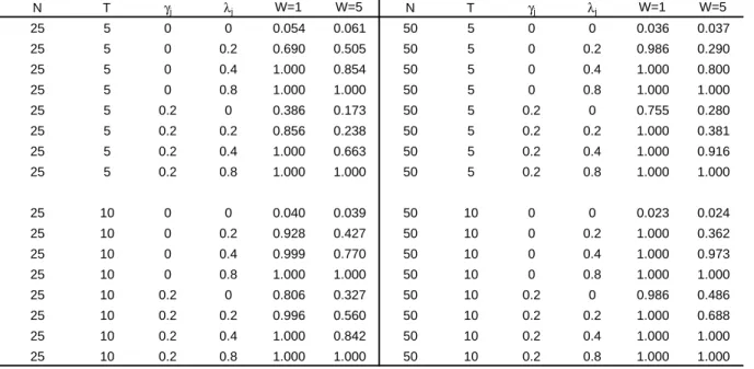
We use the same experimental design for the Monte Carlo simulations as in subsection 5.1. Table 3 gives the frequency of rejections at the 5%level for the joint LM test for Ha

0 :γj = 0, λj = 0, σµjk = 0, ∀j, k = 1, .., M = 2. For 1000 replications, counts between 37 and 63 are not significantly different from 50 at the 0.05 level. The results are reported for N = 25, 50, T = 5,

10 and for “1 ahead and 1 behind” and “5 ahead and 5 behind” weighting matrices. Table 3 shows that at the5% level, the size of the joint LM test is close to0.05and varies between0.036and0.054depending onN andT. The

we also refer to our measure as RMSE. It is defined by:

RM SE= s bias2₊ · IQ 1.35 ¸2

where bias is the difference between the median and the true value and IQ is the

in-terquantile range Q3−Q1 where Q3 is the0.75 quantile and Q1 is the0.25quantile. If

the distribution is normal, the median is the mean and, aside from a slight rounding error,

power8 _{of the joint LM test is reasonably high as long asγ}

j orλj are larger

than 0.2. In fact, if γj orλj >0.4, this power is almost one in all cases. For

a fixedγ_j orλj, this power dramatically improves as N and T increase. For

instance, for N = 25, T = 5, W = 1, λj = 0.2, the power is around 69%. If

we double T from 5 to 10, this power tends to 93%. Increasing the number of neighbors from one to five, ( i.e., W = 1 to W = 5) does not change the results significantly but slightly reduces the speed of convergence of the power to one.

5.3.2 Two-dimensional conditional LM tests

Conditional LM test for no spatial correlation and no spatial lag

given random effects Hb

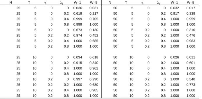
0 : γj = 0, λj = 0, ∀j = 1, .., M. Table 4 gives

the frequency of rejections at the 5% level for the two-dimensional LM test for H0b : γj = 0, λj = 0, ∀j = 1,2 (allowing σµ_jk 6= 0). In particular, we use

σ2

µ1 = 1, σ

2

µ2 = 0.5 and ρµ = 0.8. The size of this test is not significantly

different from 0.05 for N = 25, T = 5,10 and W = 1. However, it is undersized for N = 50, T = 5,10 and W = 5. The power of this LM test is reasonably high as long as γj or λj are larger than 0.2. In fact, if λj > 0.4,

this power is almost one in all cases. For a smallγj orλj,this power strongly

improves as N and T increase.

Conditional LM test for no spatial lag and no random effects given

spatial error correlation H0c : γj = 0, σµ_jk = 0,∀j, k = 1, .., M. Table 5

gives the frequency of rejections at the 5% level for the two-dimensional LM test for Hc

0 : γj = 0, σµjk = 0, ∀j, k = 1,2 (allowing λj = 0.5). For N = 25,

T = 5, the test is over-sized (0.09) but if we doubleT from5to10, or double N from 25 to 50, the size of this test becomes close to 0.05. The power of this LM test is reasonably high as long as γj is larger than 0.2. In fact, if

γj > 0.4, this power is almost one in all cases. Increasing the number of

neighbors (W = 1 to W = 5) does not change the results significantly but slightly reduces the speed of convergence of the power to one.

8_{We use the SAR specification:}

Conditional LM test for no spatial error correlation and no random

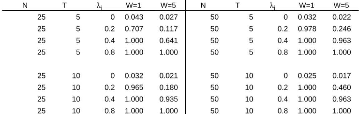
effects given a spatial lag H0d : λj = 0,σµ_jk = 0,∀j = 1, .., M. Table 6

gives the frequency of rejections at the 5% level for the two-dimensional LM test for Hd

0 : λj = 0, σµjk = 0, ∀j, k = 1,2 (allowing γj = 0.5). The size

of this test is not significantly different from 0.05 for N = 25, T = 5, but becomes slightly undersized as N, T andW increase. The power of this LM test is high as long asλj is larger than0.2. In fact, if λj >0.4,this power is

always one. Increasing the number of neighbors (W = 1 to W = 5) slightly reduces the speed of convergence of the power to one.

5.3.3 One-dimensional conditional LM tests

Conditional LM test for no spatial lag correlation given spatial

error correlation and random effects He

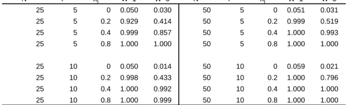
0 :γj = 0, ∀j = 1, .., M. Table

7 gives the frequency of rejections at the 5% level for the one-dimensional LM test for He

0 : γj = 0, ∀j = 1,2 (allowing σµjk 6= 0 and λj = 0.5). The

size of this test is not significantly different from 0.05 for N = 25, T = 5, but becomes slightly undersized as N, T and W increase. The power is reasonably high as long as γ_j is larger than 0.2. If γ_j > 0.4, this power is almost one in all cases. For a fixed γj, this power improves as N and T

increase. Increasing the number of neighbors (W = 1 to W = 5) slightly reduces the speed of convergence of the power to one.

Conditional LM test for no spatial error correlation given a spatial

lag and random effects H0f : λj = 0, ∀j = 1, .., M. Table 8 gives the

frequency of rejections at the 5% level for the one-dimensional LM test for H₀f :λj = 0,∀j = 1,2 (allowingσµjk 6= 0 andγj = 0.5). At the5%level, the

size of this LM test is not significantly different from0.05for all experiments involving W = 1. However, for W = 5, it becomes slightly undersized. The power is almost one as long asλj is larger than0.2. For afixedλj, this power

improves as N and T increase.

Conditional LM test for no random effects given a spatial lag and

spatial error correlation H₀g : σµjk = 0, ∀j, k = 1, .., M. Table 9 gives

the frequency of rejections at the 5% level for the one-dimensional LM test for H₀g : σµ_jk = 0, ∀j, k = 1,2 (allowing γj = 0.5 and λj = 0.5). At the 5%

σµjk 6= 0 (σ

2

µ1 = 1, σ

2

µ2 = 0.5, ρµ = 0.8) whatever the size of N andT. This

holds for both sets of W matrices considered.

6

An application to hedonic housing prices in

Paris

We illustrate our spatial panel methods by estimating a three SUR equations for hedonic housing prices in Paris. As the capital of France, Paris represents one of the most important real estate markets. The city of Paris is divided into 20 arrondissements (administrative districts) which in turn are divided into 4 quartiers (quarters). Our units of observation are the 80quartiers.

In France, the housing classification used for flats by real estate agencies and notaries is the following: the studio (or efficiency) which is the cheapest rents in a given area, and consist mainly of a large room which is the living, dining, and bedroom combined. The kitchen facilities is usually a part of this central room, but the bathroom is its own smaller separate room. The two rooms (F2) flats (or one-bedroom apartments in the US or Great Britain), in which one bedroom is separate from the rest of the apartment. The three rooms (F3) flats (or two-bedroom in the US or Great Britain), and the four rooms (F4) flats (or three-bedroom in the US or Great Britain), etc.

6.1

Data Description

The French institutional setting is characterized by a network of notaries who have a monopoly in registering real estate transactions. The data base “BIEN”, managed by the Notary Chamber of Paris covers Ile-de-France,

i.e. the city of Paris and the Paris region9. For each transaction, we have information on the price for which the property was sold, along with its detailed characteristics (size, number of rooms and bathrooms, floor level, whether it has a balcony, whether it has a garage, a maid’s room, time of construction, etc.) and its precise localization (Lambert II grid coordinates) with a precision of the order of 5 meters.

The data base covers the period 1990-2003. The dependent variable is the

9_{The data on a particular sale is made on a voluntary basis. However, the rate of}

coverage in 2003 is estimated to be 83% in Ile-de-France. Moreover, the database is

(log) mean price per square meter10_{in eachquartier for each time period and}

the explanatory variables are the mean characteristics of properties in each

quartier for each time period. Using this aggregatedquartier data gives us a balanced panel data of N T = 80_×14 = 1120 observations per variable.11

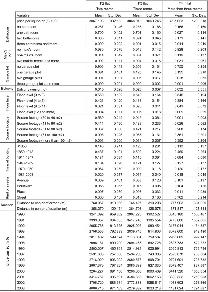
Put Table 10 here

Table 10 gives some descriptive statistics for housing prices and housing characteristics by three types of flats sold in the 80 quartiers during the period 1990₋2003. We have dropped studios, and flats with more than 8 rooms. So, the statistics pertain to flats with two rooms, three rooms and four to seven rooms (hereafter F2, F3, F4m, respectively).

The mean price per square meter is about 3000 euros, this ranged from

932 to 1200 euros per square meter. The mean price of flats has followed a J-shape curve. We observe a decrease from 1990 to 1997 and a boom after. This downswing and then upswing are more pronounced for the larger flats (F4m) and lead to mean prices per square meter between 4000 and 4400

euros.

Note that 29% (resp. 26%, 16%) of the F2 flats (resp. F3 and F4m) are not equipped with a bathroom and 70% (resp. 70%, 63% ) have one bathroom. The majority of properties are sold without a parking lot (90%,

85%,75%respectively for F2, F3 and F4m) and without a maid’s room (98%,

95%,83% resp. for F2, F3 and F4m).

Less than 3% of the flats have a balcony. These properties are mainly located between the ground floor and the third floor (55%) and only 8.4%

of buildings have more than 7 floors. The mean square footage of all the properties is around 60 m2. About 80% of these buildings are located in

10_{Our SUR ML estimator with spatial lags and spatial errors is derived only for a}

balanced panel data set with three indexes(jit)wherej = 1, ..., M equations,i= 1, ..., N

individuals (“quartiers”) and t = 1, ..., T time periods. The initial data base “BIEN”

covers more than260,000transactions and is an unbalanced clustered panel data set with

four indexes (jlit) where l = 1, ..., Li flats sold in “quartier” i(= 1, ..., N). This is why

we use mean price per square meter³PLi_l=1pjlit/Li

´

instead of price of eachflat(pjlit)of

typej in each “quartier”iat timet.

11_{Unfortunately, some variables of interest like property taxes, crime rates, etc., were}

not available in this data set at the quartier level. These unobservable characteristics of

the Paris districts may account for the spatial correlation in the disturbances and may be

streets, followed by avenues (7₋10%) and boulevards (5₋10%). The mean distance between these flats and the barycenter of each quartier is around

360 m.

Putfigure 1 here

Figure 1 summarizes the spatial localization of mean prices per square meter of properties in the Paris area. This graph reveals the spatial heterogeneous behavior of housing prices, with low prices (< 2500 euros per sq.m) for some arrondissements as XV IIIth, XIXth and XXth which are the north side popular districts of Paris and high prices (> 4000 euros per sq.m) for somearrondissements asVth_{, V I}th_{, V II}th_{, V III}th _{andXV I}th _{which are the}

famous, young, trendy and fashionable districts of Paris. Put figures 2 and 3 here

Figures 2 and 3 give the mean prices per square meter of the properties in Paris during the period 1990-2003. We observe a decrease from 1990 to 1997 and a boom after. These downswing and upswing are more pronounced for some arrondissements as Vth, V Ith, V IIth and XVth. These graphs reveal the heterogeneity in house price movements across time and quartier. Figure 3 also gives the proportion of flats according to square footage, by

arrondissement.

6.2

The model and estimation results

To our knowledge, there is no econometric study on hedonic housing prices for the Paris real estate market that uses both panel and spatial dimensions and also take into account both micro-markets and market segmentation between several kinds of flats.12

The hedonic price function describes the expected price (expressed in logs) as a function of the house characteristics described in the data section (see Rosen (1974)). However, here we generalize it by introducing both spatial lag and spatial errors:

ln (Yjt) = γjW1jln (Yjt) +Xjtβj+εjt , j = 1,2,3, t= 1, ..., T (30)

with εjt = λjW2jεjt+ujt andujt =µj +vjt.

12_{Some of the hedonic housing studies for France include Gravel et al. (1997), David et}

al. (2002), Laferrère (2003), Meese and Wallace (2003), Le Blanc and Lagarenne (2004), Maurer et al. (2004), Nappi-Choulet and Maury (2009) and Fack and Grenet (2010).

Yjt is the (N ×1)vector of mean price per square meter for time period

t = 1, ..., T and flat type j = 1,2,3. The vector of observations is over

the (N = 80) quartiers. Xjt is a (N ×kj) matrix of mean characteristics

of properties in the quartiers for time period t and flat type j. βj is a

(kj ×1) vector of parameters and εjt is an (N ×1) vector of disturbances.

µ_j is an (N _×1)vector of unobserved quartiers effects and vjt is an (N×1)

vector of remainder disturbances. In this standard SUR hedonic housing price specification, the coefficients βj measure the shadow prices of average

house attributes forflats of type j. W1j andW2j are(N ×N)spatial weight

matrices, usually containing functions of distance or contiguity relations. This is an extension of the single equation spatially autoregressive (SAR) process introduced by Cliffand Ord (1973, 1981) to the SUR case, see Anselin (1988). The vector[W1jyjt]is typically referred to as the spatial lag ofyjt. In addition

to allowing for general spatial lags in the endogenous variables, we also allow for spatial autocorrelation in the disturbances. In particular, we assume that the disturbances (εjt) are generated by a spatially autoregressive (SAR)

process. γj is the coefficient of the spatially lagged dependent variableW1jyjt,

while λj is the coefficient of the spatially correlated errors.

The Lambert II grid coordinates allow us to compute distances dpq

be-tweenflats of the same type j sold in the twoquartiers pandq. As the rela-tionship we are modelling varies over space, mean prices of transactions that are near should exhibit similar relationships and those that are more distant may exhibit dissimilar relationships. Each spatially lagged variable depends upon a weight matrix which may vary across equations: Wj =

n

w(pqj)

o

with wpp(j) = 0and the weight wpq(j) is defined bywpq(j)=d−_pq1/³PN_n=1d−_pn1

´

forp₆=q. This is row standardized, so that each row sums to1. In this case, the spatial weight matrix is filled with N(N ₋1) = 6320 nonzero elements depending on dpq.

Another possible source of locational information is contiguity, reflecting the relative position in space of one unit with respect to the other units. The spatial contiguity matrix is defined as w(pqj) = 1 for p 6= q, for entities that

share a common edge; otherwise, this weight is equal to zero. We consider here the 16 nearest neighbors (i.e. quartiers) which roughly corresponding to the4nearestarrondissements. Regarding spatial dependence, neighboring

quartiers should exhibit a higher degree of spatial dependence thanquartiers

located far apart. This contiguity matrix is also row-normalized. In this case, the spatial contiguity matrix is sparse and is filled with only 16N = 1280

nonzero elements.

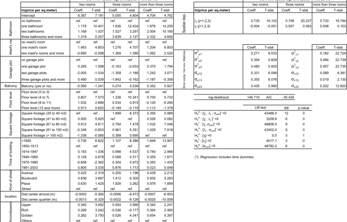
Table 11 gives the estimation results of our hedonic housing price SUR system with spatial lags and spatial errors where the weights matrices W1j

andW2j are functions of distances13. The estimated values of the spatial

de-pendence coefficients (γ1,γ2 andγ3) are not significantly different from zero. In contrast, the estimated values of the spatial autocorrelation coefficients (λ1, λ2 andλ3) are(0.735,0.756 and0.73)which are all statistically different from zero.

The estimated variance-covariance matrices of the disturbances shown in Table 11 report significant cross-correlations between the three types offlats. This is true for the unobserved quartiers effects as well as the remainder disturbances. These significant cross-correlations favor the use of a panel SUR model for hedonic housing prices in Paris.

Lagrange multiplier (LM) tests for spatial autocorrelation, spatial lags and random effects are also reported in Table 11. These LM tests do not reject zero spatial lag on the dependent variable but they do reject zero effects on the spatial autoregressive structure of the disturbances and also the zero variance-covariance effects from the random quartier effects.

In summary, with distance matrices for both spatial lags and spatial er-rors, our results seem to favor a hedonic housing price SUR system with spatial autoregressive disturbances and random quartier error components but without a spatial lag on the dependent variables.14

Put Table 11 here

Except for three specific dummies (upper, rich and golden districts) and two distances variables (distance from the center of the arrondissement and distance from the center of the quartier, which are expressed in meters), all the other explanatory variables are ratios. So, the shadow price for an attribute Xkj is computed at the average price per square meter of the flat

of type j. For F2 flats, if the demand for these flats with one bathroom increases by 10%, shadow price is expected to be, on average, 361 euros per

13_{Time dummies have been removed to save space.}

14_{As the estimated parameters bγ}

j were not statistically significant in Table 11, the

model was re-estimated by dropping the spatial autoregressive lag in yj, but not the

spatial dependence in the disturbances, see (3). The results are practically the same and are not reported here to save space. They are available upon request from the authors. They are used here to compute the shadow prices for house attributes.

square meter (hereafter e.s.m) to get this property. If the demand for F2 flats with one maid’s room increases by10%, the shadow price is around448

e.s.m. The impact of garage plot(s) is relevant for the largest F4mflats, and the shadow price is 123 e.s.m for one garage and 409 e.s.m for two garage plots, altough with wider confidence intervals. Shadow prices are expected to be higher for properties located at higher floor levels. For F2 flats, the shadow price of floor level (4 to 7) is 247 e.s.m. For F2 flats, the shadow price for larger square footage is 153 e.s.m as we go from [20m2₋40m2]

to [41m2

−60m2_{], and 279 e.s.m as we go to [61m}2

−80m2_{]. The quality} of flats is also linked to their date of construction. As compared to the reference period (1850-1913) which includes the 19th century Hausmannian construction in Paris (1852-1870), old buildings built in the previous period are strongly demanded since their shadow prices are608 e.s.m for F4mflats. The closest the flat is to the quartier (or arrondissement) barycenter, the higher is the shadow price. This price is expected to be between388and806

e.s.m less on average if the distance to the center of thequartier is increased by 100 meters. Last, living in the rich districts of Paris strongly increase the average price per square meter of all kinds of flats (around 1700 e.s.m for the F3 flats). Fashionable districts have a premium, especially “upper-class areas” (XIVth and XVth arrondissements), “rich, famous, young and trendy areas” (Vth _{andV I}th_{arrondissements) and “golden adresses” (V II}th_,

V IIIth _{andXV I}th _{arrondissements).}

For robustness checks we also used the contiguity spatial weight matrix and we get similar results but with different magnitudes. The LM tests still reject the spatial lag but not the spatial autocorrelation. These results are reported in Table 12.

Put Table 12 here

7

Conclusion

This paper proposed ML estimators for a panel SUR with both spatial lag and spatial error components. It extends the MLE approach developed by Wang and Kockelman (2007) to the general case where spatial effects are incorporated via spatial error terms and via a spatial lag on the dependent

variables and where the heterogeneity in the panel is incorporatedviaan error component specification. This panel SUR model can be estimated using an iterative three-step method.

We also considered the problem of testing for random effects as well as spatial correlation under normality of the disturbances, and proposed joint and conditional LM tests for several sources of misspecification. This ex-tends earlier work by Baltagi, et al. (2007) on spatial panels from the single equation to the SUR case.

While we did not derive the asymptotic distribution of our test statistics, we conjectured that they are likely to hold under similar set of primitive assumptions described in Kelejian and Prucha (2001). We reported extensive Monte Carlo experiments on bias and RMSE relating to the ML estimators for the SUR parameters, the variance components, the spatial lags and spatial errors coefficients for SAR and SMA process.

We find that the biases are small (less than 3%) even when N is small. These biases decrease when we double N. The results are similar for the SMA specification but, on average, bias and RMSE are smaller than those of the SAR process.

The same experimental design for the Monte Carlo simulations was used to obtain the size and power for the joint LM test, the two-dimensional conditional LM tests and the one-dimensional conditional LM tests. At the

5%level, the size of these LM tests are close to 0.05depending onN andT. The power of these tests is reasonably high as long as the spatial lag and the spatial error components are larger than0.2.

The results in the paper should be tempered by the fact that in our Monte Carlo experiments, N = 25, 50 and T = 5, 10 and we consider only two equations. One could encounter more equations, and larger N in micropanels. LargerN will probably improve the performance of these tests whose critical values are based on their large sample distributions. However, it is well known that maximum likelihood and quasi-maximum likelihood estimation of the spatial autocorrelation coefficients can be computationally difficult, particularly when N is large.

The paper concludes with an empirical illustration involving hedonic housing prices in Paris. For the 80 quartiers data for the city of Paris ob-served over the period1990₋2003,our results suggest that a reasonable spec-ification is a hedonic housing price SUR system with spatial autoregressive disturbances and random quartier effects, but without a spatial lag on the dependent variables. Using this specification, wefind statistically significant

as well as reasonable estimates of the shadow prices for mean characteristics of three types of flats considered.

References

Anderson, T., 1984. An Introduction to Multivariate Statistical Analysis, Wiley, New

York.

Anselin, L., 1988. Spatial Econometrics: Methods and Models, Kluwer Academic

Pub-lishers, Dordrecht.

Anselin, L., Le Gallo, J., and H. Jayet, 2008. Spatial panel econometrics, The

Econo-metrics of Panel Data: Fundamentals and Recent Developments in Theory and Practice, Chapter 19, L. Mátyás and P. Sevestre, (eds.), Springer, Berlin, 625-660. Anselin, L. and A.K. Bera, 1998. Spatial dependence in linear regression models with an

introduction to spatial econometrics, in Handbook of Applied Economic Statistics,

A. Ullah and D.E.A Giles, (eds.), Marcel Dekker, New York.

Arguea, N. and C. Hsiao, 1993. Econometric issues of estimating hedonic price functions,

Journal of Econometrics, 56, 243-267.

Avery, R.B, 1977. Error components and seemingly unrelated regressions,Econometrica

45, 199-209.

Baltagi, B., 1980. On seemingly unrelated regressions with error components,

Econo-metrica 48, 1547-1551.

Baltagi, B.H., 2010. Spatial panels, forthcoming in The Handbook of Empirical

Eco-nomics and Finance, A. Ullah and D.E.A. Giles, (eds.), Chapman and Hall. Baltagi, B., S.. H. Song, B. C. Jung and W. Koh, 2007. Testing for serial correlation,

spa-tial autocorrelation and random effects using panel data,Journal of Econometrics

140, 5-51.

Breusch, T.S. and A.R. Pagan, 1980. The Lagrange multiplier test and its applications

to model specification in econometrics, Review of Economic Studies47, 239-253.

Can, A., 1992. Specification and estimation of hedonic housing price models, Regional

Science and Urban Economics, 22, 453-477.

Cliff, A., and Ord, J., 1973. Spatial Autocorrelation, Pion, London.

David A., Dubujet F., Gouriéroux C. and Laferrère A., 2002. Les indices de prix des

logements anciens,Insee méthodes, Paris, 98.

Dubin, R., 1992. Spatial autocorrelation and neighborhood quality,Regional Science and

Urban Economics, 22, 433-452.

Dubin, R., Pace, K, and T. Thibodeau, 1999. Spatial autoregression techniques for real

estate data, Journal of Real Estate Literature, 7, 79-95.

Elhorst, J.P., 2003. Specification and estimation of spatial panel data models,

Interna-tional Regional Science Review,26, 244-268.

Fack, G. and J. Grenet, 2010. When do better schools raise housing prices? Evidence

from Paris public and private schools,Journal of Public Economics, 94(1-2), 59-77.

Fiebig, D.G., 2001. Seemingly unrelated regression, in A Companion to Theoretical

Econometrics, Chapter 5, Baltagi, B.H. (ed.), Blackwell, Massachusetts.

Fingleton, B., 2008a. A generalized method of moments estimator for a spatial panel

model with an endogeneous spatial lag and spatial moving average errors, Spatial

Economic Analysis,3, 27-44.

Fingleton, B., 2008b. Housing supply, housing demand and affordability,Urban Studies,

45, 1545-1563.

Glaeser, E.L., 2008. Cities, Agglomeration and Spatial Equilibrium, Oxford University

Press, Oxford.

Gravel, N., Martinez, M. and A. Trannoy, 1997. Evaluation des prix hédoniques du

loge-ment dans les communes du Val-d’Oise,Rapport pour la Direction Départementale

de l’Equipement du Val-d’Oise, THEMA-CNRS, Université de Cergy-Pontoise.

Griliches Z., 1971. Price Indices and Quality Change, Harvard University Press,

Cam-bridge, Massachusetts.

Halvorsen, R., and H. Pollakowski, 1981. Choice of functional form for hedonic price

equations,Journal of Urban Economics, 10, 37-49.

Helpman, E., 1998. The size of regions, in Public Economics, Pines, D. Sadla. E and I.

Kapoor, M., H.H. Kelejian and I.R. Prucha, 2007. Panel data models with spatially

correlated error components,Journal of Econometrics 140, 97-130.

Kelejian, H.H. and I.R. Prucha, 2001. On the asymptotic distribution of the Moran I

test with applications. Journal of Econometrics 104, 219-257.

Laferrère A., 2003. Hedonic housing price indices: the French experience, IMF and

BIS conference on Real Estate Indicators and Financial Stability, Washington, DC, October 27-28.

Le Blanc, D and C. Lagarenne, 2004. Own-occupied housing and the composition of

the household portfolio: the case of France, Journal of Real Estate Finance and

Economics, 29, 259-275.

Le Sage, J. and R.K. Pace, 2009. Introduction to Spatial Econometrics, Taylor & Francis,

New York.

Magnus, J.R., 1982. Multivariate error components analysis of linear and non-linear

regression models by maximum likelihood,Journal of Econometrics,19, 239-285.

Maurer, R., Pitzer, M. and S. Sebastian, 2004. Hedonic price indices for the Paris housing

market,Advances in Statistical Analysis (Allgemeines Statistisches Archiv), 88(3),

303-326.

Meese R. and N. Wallace, 2003. House price dynamics and market fundamentals: the

Parisian housing market,Urban Studies, 40 (5-6), 1027-1045.

Nappi-Choulet I. and T. Maury, 2009. A Spatiotemporal Autoregressive Price Index for

the Paris Office Property Market,Real Estate Economics, 37(2), 305 340.

Pinkse, J., 1998. Asymptotic properties of Moran and related tests and a test for spatial correlation in probit models. Working paper, Department of Economics, University of British Columbia.

Pinkse, J., 1999. Moran-Oavoured tests with nuisance parameters: examples, inAdvances

in Spatial Econometrics: Methodology, Tools and Applications, Anselin, L. and R.J.G.M. Florax (Eds.), Springer, Berlin, 67-77.

Nerlove, M. 1970. Further evidence on the estimation of dynamic economic relations

Rey, S.J. and M.G. Boarnet, 2004. A taxinomy of spatial econometric models for

si-multaneous equations systems, inAdvances in Spatial Econometrics: Methodology,

Tools and Applications, Anselin, L. and R.J.G.M. Florax, (eds.), Springer, New York, 99-120.

Rosen, S., 1974. Hedonic prices and implicit markets,Journal of Political Economy,82,

34-55.

Srivastava, V.K and D.E.A Giles, 1987. Seemingly Unrelated Regression Equations:

Model and Estimation, Marcel Dekker, New York.

Wang X., K.M. Kockelman, 2007. Specification and estimation of a spatially and

tem-porally autocorrelated seemingly unrelated regression model: application to crash

rates in China,Transportation,34, 281-300.

Zellner, A., 1962. An efficient method of estimating seemingly unrelated regression

equa-tions and tests for aggregation bias,Journal of the American Statistical Association,

8

Appendix: the information matrix

[I(θ)]−1 =₋E

·

∂2` ∂θ∂θ0

¸−1

is not block-diagonal betweenγ_j andλj (andγj andβ) and theI(θ)elements

are: Iββ0 = X0B0Ω−_u1BX Iβγj = X 0_B0³¡_TΩ µ+Ωv ¢−1 Fjj_⊗JT ⊗Sj ´ Xβ +X0B0¡Ω_v−1Fjj_⊗ET ⊗Sj ¢ Xβ Iβλj = 0,Iβσ_µlm = 0, Iβσ_vlm = 0 Iγjγl = T ×T r £ FjjFll¤T r£D_jADA_l ¤ +T rhβ0X0³Fll¡TΩµ+Ωv ¢−1 Fjj_⊗JT ⊗Sl0Sj ´ Xβi +T r£β0X0¡FllΩ_v−1Fjj_⊗ET ⊗Sl0Sj ¢ Xβ¤ +T rhFll¡TΩµ+Ωv ¢−1 Fjj+ (T ₋1)FllΩ_v−1FjjiT r[R_l0Rj] Iγ_jλl = T ×T r £ FjjFll¤_×T r£DjAU B l ¤ +T rhFjj¡TΩµ+Ωv ¢−1 Fll¡TΩµ+Ωv ¢i T rhRj ¡ DlB ¢0i + (T ₋1)_×T r£FjjΩ−_v1FllΩv ¤ ×T rhRj ¡ D_lB¢0i Iγjσµlm = T ×T r h Flm¡TΩµ+Ωv ¢−1 FjjiT r[Rj] Iγ_jσ_vlm = T r h Flm¡TΩµ+Ωv ¢−1 Fjj+ (T ₋1)FlmΩ_v−1FjjiT r[Rj]

Iλjλl = T ×T r £ FjjFll¤T r£D_lBD_jB¤ +T rhFll¡TΩµ+Ωv ¢−1 Fjj¡TΩµ+Ωv ¢i T rhDB_j ¡D_lB¢0i + (T ₋1)_×T r£FllΩ−_v1FjjΩv ¤ T r h DjB ¡ DlB ¢0i Iλjσµlm = T ×T r h Flm¡TΩµ+Ωv ¢−1 FjjiT r£DjB ¤ Iλjσ_vlm = T r h Flmn¡TΩµ+Ωv ¢−1 + (T ₋1)Ω−_v1oFjjiT r£DB_j ¤ Iσ_µjkσ_µlm = N T2 2 T r h Fjk¡TΩµ+Ωv ¢−1 Flm¡TΩµ+Ωv ¢−1i Iσ_µjkσ_vlm = N T 2 T r h Fjk¡TΩµ+Ωv ¢−1 Flm¡TΩµ+Ωv ¢−1i Iσ_vjkσ_vlm = N 2T r h Fjk¡TΩµ+Ωv ¢−1 Flm¡TΩµ +Ωv ¢−1 + (T ₋1)FjkΩ_v−1FlmΩ−_v1i where DAj =W A− 1 j , D B j = ½ W H_j−1 for SAR L−_j1W for SMA , U B j = ½ H_j−1W for SAR W L−_j1 for SMA Sj = ½ HjW A−j1 for SAR

L−_j1W A−_j1 for SMA andRj =

½ HjW A−j1H− 1 j for SAR L−_j1W A−_j1Lj for SMA Fjk _{is an (M}

×M) matrix of zeroes except for its (j, k)and(k, j)elements, which are equal to one. Here j, k, l and m index equations 1 through M. Derivations of the score vector and the information matrix are available upon request from the authors in the supplement material.

Table 1 - Bias and RMSE of ML estimators and standard errors of estimators Table 1 - Bias and RMSE of ML estimators and standard errors of estimators Table 1 - Bias and RMSE of ML estimators and standard errors of estimators Table 1 - Bias and RMSE of ML estimators and standard errors of estimators for panel SUR with spatial lag and spatial autoregressive errors (SAR) for panel SUR with spatial lag and spatial autoregressive errors (SAR) for panel SUR with spatial lag and spatial autoregressive errors (SAR) for panel SUR with spatial lag and spatial autoregressive errors (SAR)

bias rmse bias rmse bias rmse bias rmse bias rmse bias rmse bias rmse bias rmse

ββββ11111111 1 0.01738 0.28376 -0.00557 0.01938 0.01407 0.29966 -0.00706 0.02209 0.02211 0.17986 -0.00090 0.00817 0.00237 0.18398 -0.00130 0.00975 ββββ12121212 1 0.02729 0.21200 -0.00371 0.01417 0.02357 0.21581 -0.00401 0.01991 0.02690 0.13011 -0.00026 0.00660 0.01162 0.13721 -0.00063 0.00986 λλλλ1111 0.5 -0.00562 0.01990 0.00000 0.00336 -0.00243 0.01618 -0.00040 0.00620 -0.00539 0.01425 0.00018 0.00168 -0.00327 0.01255 0.00006 0.00334 γγγγ1111 _0.8 -0.00228 0.07582 -0.00016 0.00527 -0.04313 0.14258 0.00667 0.02194 0.00694 0.05353 -0.00040 0.00276 -0.02129 0.09120 0.00195 0.00964 σσσσ2222 µ11 µ11 µ11 µ11 1 -0.07766 0.33669 -0.02377 0.09473 -0.07991 0.34847 -0.02549 0.09808 -0.05091 0.31141 -0.01547 0.08894 -0.05717 0.31981 -0.01605 0.08963 σσσσ2222 µ12 µ12 µ12 µ12 0.56569 -0.03881 0.21092 -0.01492 0.06074 -0.04486 0.21885 -0.01521 0.06380 -0.02148 0.18879 -0.00727 0.05567 -0.02723 0.19788 -0.00893 0.05637 σσσσ2222 µ22 µ22 µ22 µ22 0.5 -0.04632 0.17166 -0.01288 0.04858 -0.04935 0.17690 -0.01420 0.05037 -0.02410 0.15524 -0.00677 0.04442 -0.02505 0.16435 -0.00758 0.04709 ββββ21212121 1 0.01499 0.19823 -0.00415 0.01383 0.01969 0.22051 -0.00699 0.01613 0.01423 0.11973 -0.00150 0.00631 0.00441 0.14076 -0.00220 0.00762 ββββ22222222 1 0.02111 0.14887 -0.00315 0.01009 0.01571 0.14981 -0.00501 0.01284 0.01559 0.09000 -0.00102 0.00474 0.00310 0.10058 -0.00211 0.00