UC San Diego
UC San Diego Electronic Theses and Dissertations
TitleReal Exchange Rates and Foreign Portfolio Investment
Permalink
https://escholarship.org/uc/item/8c11f29h
Author
Bloom, Patrick Roll
Publication Date
2019
UNIVERSITY OF CALIFORNIA SAN DIEGO
Real Exchange Rates and Foreign Portfolio Investment
A dissertation submitted in partial satisfaction of the requirements for the degree
Doctor of Philosophy in Economics by Patrick Bloom Committee in charge:
Marc-Andreas Muendler, Chair Prashant Bharadwaj James Hamilton Gordon Hanson Michael Melvin Natalia Ramondo 2019
Copyright Patrick Bloom, 2019
The dissertation of Patrick Bloom is approved, and it is acceptable in quality and form for publication on microfilm and electronically:
Chair
University of California San Diego
EPIGRAPH
The only moment of happiness possible, that’s the present. The past gives regrets. And the future uncertainty. Man understood this very quickly and invented religion. It forgives him for the evil he’s done in
the past and tells him not to worry about the future—because he’ll go to Paradise. That means, take advantage of the present.
TABLE OF CONTENTS
Signature Page . . . iii
Epigraph . . . iv
Table of Contents . . . v
List of Figures . . . viii
List of Tables . . . ix
Acknowledgements . . . xi
Vita . . . xii
Abstract of the Dissertation . . . xiii
Chapter 1 Nominal vs long-term real exchange rate volatility . . . 1
1.1 Introduction . . . 1
1.2 Definitions and foundations . . . 3
1.2.1 Pricing measure and domestic bonds . . . 3
1.2.2 Foreign bonds . . . 4
1.2.3 Inflation-linked bonds . . . 4
1.2.4 Foreign inflation-linked bonds . . . 4
1.2.5 Real exchange rate . . . 5
1.2.6 Key identity . . . 5
1.2.7 Comparison to the literature . . . 7
1.3 Empirical strategy . . . 7
1.4 Data . . . 9
1.5 Discussion of measurement . . . 10
1.5.1 CPI timing . . . 10
1.5.2 Inflation-linked bond timing . . . 10
1.5.3 Illiquidity . . . 11
1.5.4 Default Risk . . . 12
1.5.5 Inflation-floor protection . . . 13
1.6 Results . . . 13
1.7 Conclusion . . . 17
Chapter 2 An equity portfolio investment channel for real exchange rate volatility . . 19
2.1 Introduction . . . 19
2.2 Portfolio equity investment . . . 26
2.2.1 Literature on real effects of portfolio investment . . . 26
2.3 Structural breaks after equity market liberalizations . . . 37
2.4 Model . . . 38
2.4.1 Preview of model . . . 38
2.4.2 Preferences, demands, prices, and the real exchange rate . . 40
2.4.3 Production and the market for intermediate inputs . . . 41
2.4.4 Market-clearing . . . 42
2.4.5 Equilibrium . . . 43
2.4.6 Foreign investment . . . 44
2.4.7 The real exchange rate . . . 44
2.4.8 Equities valuation . . . 45
2.4.9 Productivity and signal . . . 45
2.4.10 Foreign investors . . . 46
2.4.11 Key equations . . . 47
2.5 Empirical support . . . 48
2.5.1 Quarterly portfolio investment and the nominal exchange rate 48 2.5.2 Real exchange rates and new varieties . . . 51
2.6 Parametrization and magnitudes . . . 53
2.6.1 Parameters . . . 53
2.6.2 Interest Rate Shock . . . 56
2.6.3 Volatility . . . 57
2.7 Conclusion . . . 58
Chapter 3 Foreign ownership and productivity of Chilean manufacturers . . . 59
3.1 Introduction . . . 59
3.2 Productivity measurement . . . 62
3.2.1 Production . . . 62
3.2.2 Tornqvist and Malmqvist productivity indices . . . 63
3.2.3 The Levinsohn-Petrin approach . . . 64
3.2.4 The Ackerberg-Caves-Frazer approach . . . 66
3.2.5 GMM framework . . . 67
3.3 Estimation strategy . . . 68
3.3.1 Ordinary Least Squares . . . 68
3.3.2 Local linear regressions . . . 69
3.4 Data . . . 70
3.5 Results . . . 72
3.5.1 OLS in levels . . . 72
3.5.2 Local linear regressions . . . 72
3.5.3 OLS in changes . . . 75
3.5.4 Instrumental variables . . . 79
3.5.5 Share of inputs imported . . . 81
Appendix A Appendices to Chapter 1 . . . 85
A.1 Illiquidity, robustness to maturity . . . 86
A.2 A general approach to the stochastic discount factor . . . 86
Appendix B Appendices to Chapter 2 . . . 89
B.1 Robustness of extensive margin . . . 90
B.2 Portfolio constraints . . . 90
B.3 Firms’ use of external capital . . . 91
B.4 Dynamics of flows under leverage constraint . . . 92
Appendix C Appendices to Chapter 3 . . . 95
C.1 Industry details . . . 96
C.2 Robustness to productivity measure . . . 96
C.3 Robustness to outliers . . . 98
LIST OF FIGURES
Figure 1.1: Mexican inflation-linked bond yields and smoothed par and zero real yield curves on November 30, 2012. Source: Bloomberg Finance LP and author’s calculations. . . 10 Figure 1.2: 20 year ”breakeven inflation” expectations for Mexico versus 1 yr inflation
expectations reported by the Banco de Mexico. Data from Bloomberg, FRED, national statistical agencies, and author’s calculations. . . 12 Figure 1.3: Real yields with 20 year maturity for Mexio and USA. Sample is April 2008
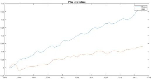
to July 2017. Data from Bloomberg, FRED, national statistical agencies, and author’s calculations. . . 14 Figure 1.4: Consumer price indices for the US and Mexico, rebased so the price level
starts at 1. Sample is April 2008 to July 2017. Data from FRED and national statistical agencies. . . 14 Figure 1.5: Exchange rates between Mexico and the United States, rebased so the
nominal exchange rate starts at 1. Sample is April 2008 to July 2017. Data from Bloomberg, FRED, national statistical agencies, and author’s calculations. 15 Figure 1.6: Exchange rates between Brazil and the United States, rebased so the nominal
exchange rate starts at 1. Sample is November 2005 to July 2017. Data from Bloomberg, FRED, national statistical agencies, and author’s calculations. . 17 Figure 2.1: Broad Real Effective Exchange Rates, May 2013 - April 2018. Rebased to
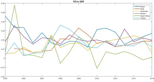
100 at May 2013. Source: Bank for International Settlements . . . 20 Figure 2.2: Foreign direct investment to GDP for select countries 2000-2016. The series
is the net incurrence of liabilities in equity securities from the IMF Balance of Payments Database. . . 30 Figure 2.3: Foreign portfolio investment to GDP for select countries 2000-2016. The
series is the net incurrence of liabilities in equity securities from the IMF Balance of Payments Database. . . 30 Figure 2.4: 30yr constant maturity real yields. Constructed by the Board of Governors
LIST OF TABLES
Table 1.1: Variance decomposition of nominal exchange rate for Mexico, Brazil, South Africa, and Turkey exchange rates versus the US. . . 15 Table 1.2: Covariance decomposition of nominal exchange rate for Mexico, Brazil, South
Africa, and Turkey exchange rates versus the US. . . 16 Table 2.1: Mean and standard deviation of monthly changes in Broad Real Effective
Exchange Rates, May 2013 - April 2018. Data from Bank for International Settlements and author’s calculations. . . 20 Table 2.2: Regression of extensive margin of imports on investment inflows and lag of
the dependent variable. . . 31 Table 2.3: Regression of extensive margin of imports on investment inflows and lag of
the dependent variable with added controls. . . 32 Table 2.4: Instrumental variables regression of extensive margin of imports on investment
inflows and lag of the dependent variable. . . 34 Table 2.5: Regression of extensive margin of intermediate input imports on investment
inflows and a lag of the dependent variable. . . 35 Table 2.6: Instrumental variables regression of extensive margin of intermediate input
imports on investment inflows and a lag of the dependent variable. . . 36 Table 2.7: Regression of extensive margin on post-liberalization indicator interactions. 38 Table 2.8: Regression of change in log exchange rate (appreciation) on lag of inward
equity portfolio investment and lag appreciation. . . 49 Table 2.9: Instrumental variables regression of change in log exchange rate (appreciation)
on lag of inward equity portfolio investment and lag appreciation. . . 51 Table 2.10: Regression of log real exchange rate change on extensive margin of imports
and investment inflows. . . 52 Table 2.11: Parameters for estimation of magnitudes. Author’s calculations. . . 53 Table 3.1: Summary statistics for manufacturing plants in Chile 1998-2001. TFP is
calculated by the Levinsohn-Petrin method with electricity use as proxy for plant-observed productivity. Plant level data from ENIA published by INE. . 71 Table 3.2: Regression of log TFP on foreign ownership . . . 73 Table 3.3: Regression of log TFP on foreign ownership with fixed effects by year, region,
and 3-digit ISIC industry code. Columns 1-5 restrict the sample to those plants with foreign ownership less than 10%, 20%, 30%, 40%, and 50% respectively. 73 Table 3.4: Local linear regression of log TFP on foreign ownership. . . 74 Table 3.5: Change in log TFP on change in foreign ownership. Fixed effects by year,
region, and 3-digit ISIC industry code. . . 75 Table 3.6: Change in log TFP on change in foreign ownership. Columns 1-5 correspond
to restricting to levels of lagged foreign ownership less than 10%, 20%, 30%, 40%, and 50%. . . 76
Table 3.7: Change in log TFP on change in foreign ownership. Sample is restricted to plants with a level of lagged foreign ownership below 10%. Columns 1-5 correspond to restricting to changes of foreign ownership less than 10%, 20%, 30%, 40%, and 50%. . . 77 Table 3.8: Change in log TFP on change in foreign ownership. Sample is restricted
to plants with a change in foreign ownership below 10%. Columns 1-5 correspond to restricting to levels of lagged foreign ownership less than 10%, 20%, 30%, 40%, and 50%. . . 77 Table 3.9: Change in log TFP on lags of changes in foreign ownership. . . 78 Table 3.10: Instrumental variables regression of log TFP level on change in foreign
ownership. . . 80 Table 3.11: Instrumental variables regression of change in log TFP on change in foreign
ownership. . . 81 Table 3.12: Instrumental variables regression of change in log TFP on change in foreign
ownership. Columns 1-5 correspond to restricting to levels of lagged foreign ownership less than 10%, 20%, 30%, 40%, and 50%. . . 82 Table 3.13: Regression of share of inputs imported on foreign ownership. Column 1
represents the full sample. Columns 2-6 restrict the sample to plants with less than 10%-50% of foreign ownership respectively. . . 83 Table 3.14: Instrumental variables regression of share of inputs imported on foreign
ownership. . . 83 Table A.1: Nominal exchange rate variance decomposition for Mexico. The long term is
10 years forward. Sample is April 2008 to July 2017. . . 86 Table A.2: Nominal exchange rate variance decomposition for Brazil. The long term is
10 years forward. Sample is November 2005 to July 2017. . . 86 Table A.3: Nominal exchange rate variance decomposition for South Africa. The long
term is 10 years forward. Sample is September 2011 to July 2017. . . 86 Table B.1: Regression of extensive margin of imports on investment inflows and lag of
the dependent variable, using a 5% threshold. . . 90 Table B.2: Regression of extensive margin of imports on investment inflows and lag of
the dependent variable weighted by their GDP. . . 91 Table B.3: Regression of portfolio equity investment on lagged equity returns. . . 92 Table C.1: Industry classifications in ENIA dataset. Source: INE. . . 96 Table C.2: Change in log TFP on change in foreign ownership with ACF measure of TFP. 97 Table C.3: Change in log TFP on change in foreign ownership with Tornqvist measure of
TFP. . . 97 Table C.4: Change in log TFP on change in foreign ownership with Tornqvist measure of
ACKNOWLEDGEMENTS
Thanks to my advisor Marc Muendler for all of the guidance. Thanks also to my committee for helpful comments.
Above all, thank you to my best friends for making this life worth living: Tim Cussins, James Dent, Luke Egeler, Paul Hanly, Ben Jackson, Rob Laragh, Mike Thornley, and Diego Vera.
VITA 1982 Born in Pasadena, California
2002 B. S. in Physicswith highest honors, University of Texas at Austin 2002 B. A. in Economics and Mathematicswith highest honors, University of
Texas at Austin
2003 M. Sc. in Economicswith merit, London School of Economics
ABSTRACT OF THE DISSERTATION
Real Exchange Rates and Foreign Portfolio Investment
by
Patrick Bloom
Doctor of Philosophy in Economics
University of California San Diego, 2019
Marc-Andreas Muendler, Chair
Chapter 1 uses real interest rates to show that the long-term real exchange rate and a risk premium are more volatile than the nominal exchange rate for four developing countries. Chapter 2 finds country-level effects of foreign portfolio investment in 18 developing countries and proposes a channel for real exchange rate volatility driven by foreign portfolio investment. Chapter 3 shows that there are plant-level productivity gains in Chile from small levels and small increases in foreign ownership typical of portfolio investment.
Nominal exchange rate changes can be decomposed into inflation differentials and real components, each having different causes and consequences. Although we have explanations for each component, the relative importance of the long-run real exchange rate has previously not
been quantified. Chapter 1 uses inflation-linked bond data for Brazil, Mexico, South Africa, and Turkey to quantify the contribution of those components to exchange rate changes against the United States. We find that the long-term expected real exchange rate plus its risk premium is even more volatile than the nominal exchange rate.
Volatility and unforecastability of real exchange rates is a fundamental puzzle of inter-national economics, and these features are even more pronounced in developing countries. In chapter 2, we present a new fact, that inward portfolio investment in equities predicts the extensive margin of imports in 18 developing countries. With this we build a purely real model in which foreign investors finance new intermediate inputs and increase productivity in the tradeable goods sector. We express the Balassa-Samuelson determined real exchange rate as a function of foreign investment. We use the established fact that investors in developed countries exhibit positive feedback or operate under portfolio constraints and show how therefore the real exchange rate reacts positively to equity prices. We test and confirm the prediction of the model that equity portfolio investment predicts exchange rates at quarterly frequencies. We also confirm that the extensive margin of imports comoves with the real exchange rate at annual frequencies, and do not reject that equity portfolio investment acts through this channel only.
In chapter 3, we measure the effect of foreign ownership on the productivity of Chilean manufacturers between 1998 and 2001. Total factor productivity is measured at the plant level using multiple alternative methods. Both the level of foreign ownership and increases in foreign ownership are significant predictors of productivity. These effects remain when restricting the sample to plants with low foreign ownership and small changes in foreign ownership, showing the importance of foreign portfolio investment on productivity. A non-parametric fit suggests that low levels of foreign ownership are as significant as larger stakes. When controlling for endogeneity in the foreign investment decision by instrumenting with total developed countries’ portfolio outflows the positive effects on productivity remain. Finally we show that foreign ownership predicts that firms source more of their intermediate inputs from abroad.
Chapter 1
Nominal vs long-term real exchange rate
volatility
1.1
Introduction
The exchange rate between two currencies determines the relative price of domestic goods and assets between the two countries. Exchange rate changes are therefore a combination of differentially changing domestic price levels and a changing relative price level. This paper quantifies the importance of the first, nominal, contribution, and the second, real, contribution.
Standard expositions of exchange rate determination rely primarily on differential inflation, uncovered interest parity, and purchasing power parity. By design those approaches ignore the violation of purchasing power parity, even though it is known to be large and persistent (Rogoff 1996.) The real exchange rate for traded goods may even be as volatile as for non-traded goods (Engel 1999).1
1Engel (1999) demonstrated this for the US exchange rate versus several developed countries using five different
metrics for traded goods prices. Further work documenting this fact across many currency pairs by Betts and Kehoe (2008) used sectoral gross output deflators or producer price indices for traded goods prices, whereas Burstein, Eichenbaum, and Rebelo (2006) used a weighted average of import and export price indices for developed countries. Yepez and Dzikpe (2019) extend Engel’s methods to developing countries with similar results.
The standard exchange rate model in small, open economy macroeconomics (illustrated in e.g. Chari, Kehoe, and McGrattan 2002) is that monetary shocks interact with sticky prices. In this model, a positive monetary shock with fixed prices increases output and depreciates the currency, and then as prices adjust the real exchange rate returns to its previous level under presumed relative purchasing parity. This mean-reversion implies that the long-term expected real exchange rate would be much less volatile than the current nominal exchange rate. We provide evidence against this theory.
Earlier empirical work by Mussa (1986) founds that real exchange rates were less volatile under fixed nominal regimes than under floating nominal exchange rate regimes. He concluded that sticky prices were the dominant mechanism. However, we find that these inflation-linked bond markets do not agree that real exchange rate volatility is transient and mean-reverting as sticky prices adjust.
Real exchange rate changes between advanced economies are humped-shaped in that they are initially persistent and then mean reverting. Burstein and Gopinath (2014) document that the half-lifes of those real exchange rate changes are between 1.5 and 6 years. This would imply that current real exchange rate changes would not greatly influence very long-term expectations because current changes largely die out over time.
Clarida (2012) studies daily currency fluctuations between the dollar and the pound, euro, and yen. He assumes a constant long-term expected real exchange rate, and attributes all variation to the risk premia. This amounts to assuming that future relative purchasing power parity holds over the sample.2 This paper instead examines countries where neither absolute nor relative PPP is expected versus the US. This is a richer problem in exchange rate economics.
The contribution of this paper is to solve for the expected long-term real exchange plus its risk premium as a function of observables, assuming only no-arbitrage, and then to quantify this component with market data. We find that the long-term expected real exchange rate plus its risk
premium is even more volatile than the nominal exchange rate.
The rest if this paper is organized as follows. Section 2 shows the financial math relating exchange rates, price levels, real yields, and expectations. Section 3 discusses how we will apply this framework. Section 4 describes the sources for data. Section 5 covers possible complications or problems. Sections 6 reports the results. And section 7 concludes.
1.2
Definitions and foundations
1.2.1
Pricing measure and domestic bonds
Any asset with uncertain payoffxT can be priced as
xt=Et 1 ItmTxT = 1 ItEt[mTxT], (1.1)
whereIt is the gross nominal interest rate between periodstandT, andmT is the pricing kernel or stochastic discount factor (following e.g. Harrison and Kreps 1979). The existence of thismT
follows only from no-arbitrage and its uniqueness from market completeness, or that all of these assets are tradeable. In this paper, we will be careful to sub-script all variables such that zs is
F
s-measurable, whereEsindicates an expectation conditional with respect toF
s. Et[mT] =1 andmT is non-negative almost everywhere, so we can definemT = ddQP as a Radon-Nikodyn derivative
and rewrite the pricing formula as
xt =EQt 1 ItxT = 1 ItE Q t [xT]. (1.2)
Actual expectations are formed under the physical probability measurePwhereas the risk-neutral measureQprices assets.
payoffIt.
1.2.2
Foreign bonds
The nominal exchange rate Et is expressed in units of domestic currency per foreign
currency. Therefore an increase inEtrepresents an appreciation of the foreign currency.
Applying the pricing formula to one foreign bond from the perspective of a domestic investor we get Et =EQt 1 It It∗ET = I ∗ t ItE Q t [ET] (1.3)
whereIt∗ is the gross nominal interest rate on foreign bonds betweent and T. This relation is what we know as “Uncovered Interest Parity.”
1.2.3
Inflation-linked bonds
An inflation-linked bond pays a certain real returnRt multiplied by the increase in the
price levelΠT, whereΠT =PT/Pt. 3
Therefore the pricing formula applied to a domestic inflation-linked bond is
1=EQt 1 ItRtΠT = Rt It E Q t [ΠT]. So EQt [ΠT] = It Rt . (1.4)
1.2.4
Foreign inflation-linked bonds
A foreign inflation-linked bond pays a certain real returnR∗tmultiplied by the increase in the price levelΠ∗T, whereΠ∗T =PT∗/Pt∗.
3To be clear, (nominal) bonds pay a certain nominal return, which is risky in real terms. Inflation-linked bonds
The pricing formula gives us Et=EQt 1 ItR ∗ tΠ∗TET =R ∗ t It E Q t [Π∗TET]. (1.5)
1.2.5
Real exchange rate
The real exchange rateQt for the foreign consumption basket with respect to the domestic
is Qt =EtP ∗ t Pt . (1.6)
So real exchange rate growth follows as
QT Qt = ET Et Π∗T ΠT . (1.7)
1.2.6
Key identity
Rearranging (1.7) and taking expectations we get
EtEQt [QTΠT] =QtEQt [ETΠ∗T].
The expectation on the right-hand side appeared earlier in pricing the foreign inflation-linked bond (1.5), so we can replace it and state
EQt [QTΠT] =Qt
It R∗t .
Now we use the pricing formula for the domestic inflation-linked bond (1.4) to substitute forIt
and stateQt as a function of real returns and expectations:
Qt= R∗t Rt EQt [QTΠT] EQt [ΠT] .
Plugging this expression for the real exchange rate into the definition of the real exchange rate (1.6) we can solve for the nominal exchange rate:
Et= Pt Pt∗ R∗t Rt E Q t " QT ΠT EQt ΠT # . (1.8)
This is a sort of “Real Uncovered Interest Parity” relation.
We are interested in the true expected long-term real exchange rate, which we will call
QEt =EP
t [QT]. The expectation (1.8) can be rewritten as
Et= Pt Pt∗ R∗t RtQ E t Θt, (1.9)
which definesΘt, a risk-premium term.4. It is important to note, that even a risk-neutral investor,
where the risk-neutral probability measureQis almost everywhere equal to the physical measure P, could haveΘ6=1 because of the possible covariance between the real exchange rate and the
domestic inflation rate. On the other hand, in our application we are interested in the covariance between US inflation and, for example, the real exchange rate with Turkey. We expect this to be zero.
Taking logs of both sides, and denoting logs of uppercase variables by their lowercase,
et= pt−p∗t +rt∗−rt+qEt +θt. (1.10)
Finally taking differences in time we have
∆et=πt−π∗t +∆rt∗−∆rt+∆qEt +∆θt, (1.11)
where∆is the difference betweent−1 andt in a monthly series.
It is worth stressing that this decomposition has relied only upon the assumption of
no-4Specifically,Θ t=1+Q1E t CovP Q T, dQ dPΠT EPt hd Q dPΠT i !
arbitrage. Nor have we required any assumptions about the form of the pricing measure. This is in contrast to Clarida (2012) who assumes that the pricing measure is homogeneous in the domestic price level.
1.2.7
Comparison to the literature
Clarida (2012) presents results for developed countries’ exchange rates by plotting et
versus pt−p∗t +r∗t −rt. He calls the latter the “risk-neutral fair value.” Following from 1.10 the difference is qtE+θt. Arguably, for similar, large, and economically-integrated developed
countries it may be reasonable to assume thatqEt is constant and thatθt is significant and volatile.
However, for smaller, poorer, countries that are distant to US investors,θt should be close to zero,
andqtE explains the difference.
Imakubo, Kamada, and Kan extend the Clarida framework assuming investors expectations of the real exchange rate is formed as the HP-filter of historical observations. We take the opposite approach and require fewer assumptions.
1.3
Empirical strategy
In this paper, we use the US Dollar as the domestic currency and examine, as foreign currencies, the Mexican Peso, Brazilian Real, South African Rand, and Turkish Lira.5
The notation above usedt andT for the two time periods. We will call these today, and the long-term. The long-term will be 10-20 years depending on the data. Given that the real rate yield curve is typically flat between 10 and 20 years maturities the differences are arguably of minor economic importance.6
5This sample of countries is not random; these are the only developing countries that issue inflation-linked bonds.
This reflects some financial competence on the part of the debt management agency in these countries. On the other hand, they may be issuing inflation-linked bonds because investors are wary of high inflation in that currency. We acknowledge these competing selection effects may be present.
The changes denoted by ∆ will be interpreted to be monthly, reflecting the frequency
of CPI measurement by national statistical agencies. Accordingly we will perform a variance decomposition of monthly exchange rate changes.
Exchange rates, inflation rates, and real yields from inflation-linked bonds are all easily observable. These will allow us to jointly construct a monthly series for the sum ∆qEt +∆θt.
Disentangling those two components would require some stricter assumptions, which we forego in the interest of generality.7
There is a strong argument thatΘt is close to 1, so thatθt is near zero. This would follow
if the long-term real exchange rateQT is independent of both the stochastic discount factor and the domestic inflation rate. The first condition holds if US investors’ marginal utilities vary independently of, for example, the prospects of South African mining operations. The second condition holds if over the long term, US inflation varies little with the real economy of Brazil. Consequently, it is economically difficult to justify a large θt. To proveθt =0 follows from
independence, return to (1.8) and apply the law of iterated expectations to
EPt QT mTΠT EPt(mTΠT) = EthEthQTEmTΠT t(mTΠT) |mT,ΠT ii (1.12) = EthQTEth mTΠT Et(mTΠT) |mT,ΠT ii =Et[QT]
Once we have time series forπt−π∗t +∆rt∗−∆rt and for∆qtE+∆θt, we can use (1.11) to
decompose the variance of∆et as
Var(∆et) =Var(πt−πt∗+∆rt∗−∆rt) +Var(∆qEt +∆θt) +2Cov(πt−π∗t +∆r∗t −∆rt,∆qtE+∆θt).
(1.13) A similar decomposition applies to the nominal exchange rate as a levelet,following from (1.10).
10 and 20 years averaged 70 basis points with a standard deviation of 37 bps. Furthermore, all results at 20 year maturity are reproduced at 10 years maturity as a robustness check in appendix A.1.
7One approach could be to parametrize the pricing kernel. In appendix A.2 we outline a general approach for
A second decomposition uses the identity
Var(∆et) =Cov(∆et,Πt−Πt∗+∆rt∗−∆rt) +Cov(∆et,∆qtE+∆θt) (1.14)
and similarly in changes. When we divide through byVar(∆et)(in our case we normalize it), the terms on the right hand side are like regression coefficients that must sum to 1. In this case they can be interpreted as how well∆et explains its constituents.
1.4
Data
Long-term real yield data for the US is collected by the Federal Reserve, cleaned with the method of Gurkaynak, Sack, and Wright (2010), and available at
https://www.federalreserve.gov/econresdata/default.htm.
Real yield data for Brazil, Mexico, South Africa, and Turkey is available from Bloomberg Finance L.P. We use month end yields and spline a real-yield par curve at each date. This par curve represents the yields of coupon-paying bonds. Splining a curve is standard practice to smooth over any bond-specific idiosyncrasies. We then convert the resulting par curve to a zero curve, from which we can select a fixed maturity. Figure 1.1 shows the results of this approach for Mexican inflation-linked bonds on November 30, 2012 (the midpoint of the sample).
Exchange rates are from the St. Louis Federal Reserve’s FRED database, as is US CPI. The Brazilian CPI (called IPCA) is from the website of the Brazilian statistical agency (IBGE.) The Mexican CPI (INPC) is from Banco de Mexico. The South African CPI is from Statistics South Africa. The Turkish CPI is from the Turkish Statistical Institute. All of these consumer price indices are reported and analyzed as monthly series.
Figure 1.1: Mexican inflation-linked bond yields and smoothed par and zero real yield curves on November 30, 2012. Source: Bloomberg Finance LP and author’s calculations.
1.5
Discussion of measurement
1.5.1
CPI timing
CPI for a month is measured throughout that month and then published sometime in the following month. In this paper we assume that the CPI is known by market participants at the end of the measurement month and the exchange rate is priced accordingly.
1.5.2
Inflation-linked bond timing
For settlement purposes, inflation-linked bonds trade with respect to a reference CPI, which is the CPI 3 months earlier, and interpolated between months. This means that the relevant price levels in the inflation-linked bond pricing-formula are actually mis-timed by 3 months. We can add a correction for this. We haven’t done that, but it is tiny, because 3 months of inflation is small versus the future inflation over the 20 year life of the bond. Gurkaynak, Sack, and Wright (2010) ignore this when reporting expected future inflation on the Federal Reserve website. If the inflation observed since the reference CPI is the same as it is expected to be in the future, then
this correction would be zero.8
1.5.3
Illiquidity
One possible objection to this approach is that these markets for inflation-linked bonds are relatively illiquid. However, we expect there exists a marginal investor willing to buy cheap assets. So the illiquidity objection is a rejection of the weak form of the efficient markets hypothesis. More generally, we can only ask what the market expects based on observable prices. Those expectations may be wrong ex-post or strange ex-ante.
Figure 1.2 plots the 10 year “breakeven inflation” computed as the difference between the nominal and real yields on Mexican nominal and inflation-linked government bonds versus the mean 1 year inflation expectations from Banco de Mexico’s business conditions survey. The co-movement is evidence that the inflation-linked bond market tracks reported expectations. If anything, the correlation is higher than we might expect, suggesting that current inflation is assumed to last long into the future.
One possible manifestation of illiquidity could be prices that update infrequently because the bonds are not being traded on a given day. We would expect this problem to be more prevalent for 20 year maturities than for 10 year, and also to be more significant earlier in the time series because of the financial crisis of 2008. Appendix A.1 shows results for the 10 year maturities that are substantively similar to those for the 20 year maturities. Furthermore, figures 1.5 and 1.6 show similar behavior for the long-term real exchange rate plus risk premium in 2008-2009 and in 2012-2016. Consequently, we conclude that the results are not driven by stale prices on illiquid bonds.
8Specifically, this correction would be to the real yield, and the magnitude is the difference between expected
Figure 1.2: 20 year ”breakeven inflation” expectations for Mexico versus 1 yr inflation expectations reported by the Banco de Mexico. Data from Bloomberg, FRED, national statistical agencies, and author’s calculations.
1.5.4
Default Risk
If there were a serious possibility of default on these bonds then the yields would carry some premium. No country has defaulted on bonds issued in a currency they can print since Russia in 1998, which was a special case (the local currency debt was largely held by foreign investors, including Long Term Capital Management). The US has occasionally threatened to default in the last few years but in those episodes US bonds have actually gone up in price.
The credit default swap (CDS) market shows a probability of default for these countries, but this is somewhat technical. The CDS reflects the probability of a credit event and a recovery rate on the lowest valued deliverable security. Say for example, if Turkey defaults on a euro-denominated bond for political reasons and continues payments on its local-currency bonds. Then the buyer of protection uses the CDS to deliver the defaulted euro-denominated bond to the seller of protection. The local-currency bonds would be unaffected. Therefore the CDS market hugely overstates the probabilities of credit events in local-currency markets.
high inflation. This would lead the market to under-price inflation because full repayment is less likely in that scenario. Therefore the market-implied expected long-term real exchange rate would be lower than the true (physical measure) expectation. We admit that these “peso problems”, or unobservable risks, are possible but doubt that they are significant factors in pricing. Either way they would affect theθt term and not the results we present.
The key results of this paper concern the volatility and not the level of the long-term real exchange rate. If default or capital controls are more likely under high inflation, then that would slow the market from pricing high inflation. This would reduce the volatility of the long-term real exchange rate. So if these concerns are salient, our results are conservative estimates of the volatility of the long-term real exchange rate, which we will find to be dominant.
1.5.5
Inflation-floor protection
Most inflation-linked bonds have a built-in floor. This means that investors are protected in case of deflation over the life of the bond. 20 years of deflation in the developing countries we study has not happened in recent history and we assume the risk of this in the future is assessed as low by market participants. In the US, the value depends on when exactly the bond was issued. Over the long term this risk must be small. Therefore we use 20 year real yields for the US without worrying about adjusting for the possibility of 20 years of deflation.
1.6
Results
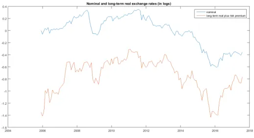
Figure 1.3 plots the log of the gross 20 year real yields for Mexico and the US, which are
randr∗in equation 1.10. Figure 1.4 plots the evolution of the price levels, or CPI, in Mexico and the US. Figure 1.5 plots the result of the decomposition, following equation 1.10, of the nominal exchange and the expected long-term real exchange rate plus its risk premium. Of note is that the latter is more volatile than the former. Furthermore, the market always expects a real depreciation
Figure 1.3: Real yields with 20 year maturity for Mexio and USA. Sample is April 2008 to July 2017. Data from Bloomberg, FRED, national statistical agencies, and author’s calculations.
over the next 20 years.
Figure 1.4: Consumer price indices for the US and Mexico, rebased so the price level starts at 1.
Sample is April 2008 to July 2017. Data from FRED and national statistical agencies.
Table 1.1 reports the variance decomposition in levels and monthly changes for Mexico, Brazil, South Africa, and Turkey. The variance of the nominal exchange rate for each country has been normalized to 100 for both levels and changes. The long-term is defined as 20 years for the
Figure 1.5: Exchange rates between Mexico and the United States, rebased so the nominal exchange rate starts at 1. Sample is April 2008 to July 2017. Data from Bloomberg, FRED, national statistical agencies, and author’s calculations.
Table 1.1: Variance decomposition of nominal exchange rate for Mexico, Brazil, South Africa,
and Turkey exchange rates versus the US. The long term is 20 years forward, except for Turkey where it is 10 years forward. Sample is April 2008 to July 2017 for Mexico, November 2005 to July 2017 for Brazil, September 2011 to July 2017 for South Africa, and April 2010 to July 2017 for Turkey, in all cases the sample start is determined by data availability. Data are normalized such thatvar(et) =100 for each row. Data from Bloomberg, FRED, national statistical agencies,
and author’s calculations.
var(qEt +θt) var(pt−p∗t −rt+rt∗) cov(qtE+θt,pt−p∗t −rt+rt∗)
Mexico levels 137 21 -29
changes 496 362 -379
Brazil levels 117 47 -32
changes 356 189 -222
South Africa levels 28 36 18
changes 208 92 -100
Turkey levels 31 40 14
changes 256 189 -172
first three countries and as 10 years for Turkey.
For all four countries, the long-term real exchange rate plus its risk premium is more volatile than the nominal exchange rate, where volatility is defined as the variance of the changes.
For Mexico and Brazil,qEt +θt varies more than the nominal exchange rate,et, in levels. For
South Africa and Turkey on the other hand, qEt +θt varies less than et in levels, suggesting
mean-reversion in the changes of the former.
Table 1.2 reports the covariance decomposition, where the two columns of course sum to the normalized variance 100. The same key facts are apparent: that the real exchange rate plus the risk premium is the dominant contributor to variance of changes (volatility) in all countries, and that South African and Turkey are qualitatively different in levels.
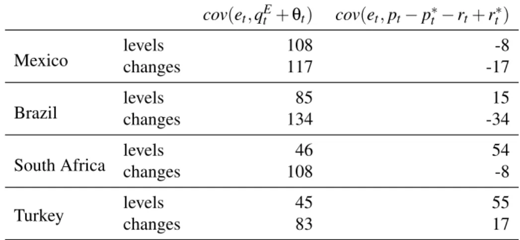
Table 1.2: Covariance decomposition of nominal exchange rate for Mexico, Brazil, South
Africa, and Turkey exchange rates versus the US. The long term is 20 years forward, except for Turkey where it is 10 years forward. Sample is April 2008 to July 2017 for Mexico, November 2005 to July 2017 for Brazil, September 2011 to July 2017 for South Africa, and April 2010 to July 2017 for Turkey, in all cases the sample start is determined by data availability. Data are normalized such thatvar(et) =100 for each row. Data from Bloomberg, FRED, national
statistical agencies, and author’s calculations.
cov(et,qEt +θt) cov(et,pt−p∗t −rt+rt∗)
Mexico levelschanges 108117 -17-8
Brazil levelschanges 13485 -3415
South Africa levelschanges 10846 54-8
Turkey levels 45 55
changes 83 17
Figure 1.6 plots the time series of the decomposition for Brazil. It is interesting to note that, for example, the depreciation of the Brazilian Real in 2015 was driven by the long-term real exchange rate. Relative to the US dollar, the currency is always (over our whole sample) expected to depreciate in real terms over the next 20 years.
Figure 1.6: Exchange rates between Brazil and the United States, rebased so the nominal exchange rate starts at 1. Sample is November 2005 to July 2017. Data from Bloomberg, FRED, national statistical agencies, and author’s calculations.
1.7
Conclusion
Real exchange rate volatility may be the fundamental puzzle of international macro-economics (Chari, Kehoe, and McGrattan 2002.) Real exchange rates are the long-term, conceptual determinants of exchange rates outside of hyper-inflationary episodes. For the exchange rates between the United States and Brazil, Mexico, South Africa, and Turkey, the long-term real exchange rate and risk premium contribute more than double the variance to monthly changes in nominal exchange rates.
This evidence reinforces to the “exchange rate determination puzzle” in which exchange rates vary considerably more than fundamentals, and which may be explained by, for example, heterogeneity of beliefs (Bacchetta and van Wincoop 2006.) This evidence is inconsistent with the standard open economy macroeconomics explanation of sticky prices and monetary shocks. After a monetary shock, these models predict prices will adjust slowly so that the real exchange will mean revert to a level determined by fundamentals.
long-term real rate is significant. It is, more nearly, that the expected long-term real exchange rate is the only thing that matters.
Chapter 2
An equity portfolio investment channel for
real exchange rate volatility
2.1
Introduction
Exchange rates are volatile and move more than forecast by standard existing models (the sixth puzzle of Obstfeld and Rogoff, 2000.)1 Accounting for inflation differentials it is variation in the real exchange rate, or the ratio of price levels between countries, that is particularly difficult to explain. In other words, relative price levels are neither stable nor mean-reverting.
In figure 2.1, we plot real exchange rates for six developing countries and the United States over a five year period (taken from the BIS and normalized to show only changes.) Table 2.1 shows the standard deviation of monthly real exchange rate changes for each country. Ignoring trends, developing countries’ real exchange rates are more volatile than for the US, by roughly a factor of two. So the fundamental puzzle of real exchange rates is even more pronounced in these countries. A key distinction is that developing countries have lower productivity and price
1“The central puzzle in international business cycles is that fluctuations in real exchange rates are volatile and
persistent.” So state Chari, Kehoe, and McGrattan 2002 in the first sentence of their abstract and then again in the first sentence of their paper.
Figure 2.1: Broad Real Effective Exchange Rates, May 2013 - April 2018. Rebased to 100 at May 2013. Source: Bank for International Settlements
levels, and therefore can either catch up or fall back in relative terms to the US. The US on the other hand is near the technological frontier and makes productive advances through an entirely different mechanism.
Developing countries interact commercially with developed countries with trade in goods and with financial investment flows, both of which may facilitate changes in productivity. Financial flows dominate the discussion of economic outcomes in developing countries in the
Table 2.1: Mean and standard deviation of monthly changes in Broad Real Effective Exchange
Rates, May 2013 - April 2018. Data from Bank for International Settlements and author’s calculations. (1) (2) mean std dev United States 0.24% 1.09% India 0.11% 1.53% Indonesia -0.15% 1.97% Mexico -0.36% 2.25% Turkey -0.54% 2.41% South Africa 0.05% 2.99% Brazil -0.20% 3.33%
popular and financial press. However in most international economic models prices adjust without any transactions taking place. Given the scale of financial flows and documented effects at the firm level, it is natural to investigate their importance at the country level.2 We fill this gap by providing a real model that incorporates foreign investment, new trade, and exchange rate determination.
We use import customs data from the UN Comtrade database, classified by the Harmonized System at the 6-digit level, and international investment flow data from the IMF’s Balance of Payments Database for the years 2000-2016. We document that equity portfolio investment predicts the extensive margin of imports in developing countries. We furthermore control for endogeneity of the equity portfolio investment, by instrumenting for recipient inflows with equity portfolio outflows from large developed countries, weighted by trade shares to the recipient countries, and find similar results. We use the classification of imports into Broad Economic Categories provided by the UN and find that more than 90% of the new imports predicted were intermediate or capital goods.
Then we look at older episodes of equity market liberalizations and import data classified by the SITC system at the 5-digit level. We test for a structural break in the growth rate of the extensive margin of imports and find that it increased (formally, we reject the null hypothesis that it stayed the same.) This new fact, that equity portfolio investment finances new imports at the country level forms the foundation of the model. In an appendix we also tests and confirm the already established fact that equity portfolio investment is procyclical with respect to equity returns in these countries. We use this to motivate the inclusion of a portfolio or leverage constraint in the model.
This paper presents a purely real model of the exchange rate in which foreign investment finances imports of new intermediate goods. These intermediate goods are used to make tradeable goods more productively. We don’t require transport costs and therefore tradeable goods have
one price globally. The real exchange rate is determined by the relative price of nontradeable goods, as in the Balassa-Samuelson effect (both 1964). Furthermore the real exchange rate moves with relative national incomes, known as the Penn effect. We choose to model this way in order to capture the economically beneficial effects of foreign investment.
In order to richen the dynamics we assume that foreign investors face a leverage constraint. To build an information channel into the model we assume there is an information signalling mechansim about future productivity in order to generate equity price volatility. The leverage constraint for foreign investors causes feedback from equity prices into investment, productivity, and thus the equilibrium exchange rate. The endogenous amplification of volatility explains why real exchange rates move as much as they do.
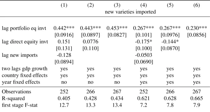
The first key test we perform is a regression of nominal exchange rates on portfolio equity investment at the quarterly frequency, where we find predictability. The second test is a regression of the real exchange rate on new varieties of imports, where we find comovement, and on lagged portfolio equity investment, where we do not reject that it is insignificant other than via new imports. We then parametrize the model and ask how important this channel is for transmiting equity price volatility to exchange rate volatility and for the effect of a rise in the world real interest rate on real exchange rates.
The contributions of this paper are to 1) document the real effects of portfolio equity investment on new imports, 2) solve a real model in which foreign investment appears explicitly in the closed form solution for the real exchange rate, and 3) illustrate the connection between equity prices and real exchange rates. This solves the puzzle that developing countries exchange rates react to the world real interest rate, and not just to interest rate differentials, as predicted by uncovered interest parity. 3
The model is entirely real, so is distinct from mechanisms in which the central bank is at fault for all crises. Furthermore, although bad loans or other problems in the banking system
3Developing countries’ currencies’ generalized depreciations between 2013 and 2017 are largely attributed to
can obviously cause a crisis, the mechanism in this paper operates independently of anything happening in a domestic banking system. The model ascribes real effects to portfolio flows, and offers a closed form expression for the real exchange rate. Several empirical facts corroborate the model’s mechanisms and implications.
This paper contains elements from international trade, macroeconomics, and finance, and consequently builds upon several distinct literatures.
A long-studied question has been the relationship between trade and growth and the direction of causation. Frankel and Romer (1999) suggest that trade itself causes growth at the macro level. Both Romer (1990) and Grossman and Helpman (1991) modeled growth as the creation of new intermediate inputs, which we use to make the connection between portfolio investment and productivity via new intermediates. Feenstra and Kee (2008) examine the relationship between export variety and country productivity, whereas we flip this and think about imported input variety determining productivity.
Leverage constraints are understood as a source of amplification and contagion of falling asset prices by Pavlova and Rigobon (2008), however changing the market price of an endowment stream is a relatively small and uninteresting effect compared to understanding the large real fluctuations in those countries. We show how leverage constraints connect prices to financial flows to real outcomes.
A large literature focuses on crisis episodes in developing countries and seeks to explain the prevalence of those episodes. The first point is that borrowing in a foreign currency makes depreciations worse for the borrower, and being forced to borrow in foreign currency is typically called the “original sin” of developing countries. Eichengreen and Hausmann (1999) suggest that foreign currency borrowing creates financial fragility and can be avoided by developing deeper domestic credit markets to allow local currency borrowing. Tirole (2003), however, argues that foreign currency borrowing is optimal because it commits the country to avoid depreciation at the expense of creditors. We do not consider debt at all and target a completely distinct mechanism.
The existing literature on third-generation currency crises that arose after the Asian crisis of 1998 typically has domestic firms borrowing in foreign currency to finance production (e.g. Aghion, Bacchetta, and Banerjee 2001 or Corsetti and Pesenti 2001.) A shock to production, the interest rate, or the exchange rate can then lead to default or depreciation via a drop in domestic money demand. However, in these cases, optimal monetary policy can prevent the devaluation and the default. This is the international crisis equivalent of Friedman and Schwartz’s conclusion that the Great Depression was, as Ben Bernanke put it, essentially the central bank’s fault.4 This paper argues that any less-developed country open to capital flows may experience real exchange rate volatility independent of monetary policy.
The standard explanation in small, open economy macroeconomics is illustrated in Chari, Kehoe, and McGrattan (2002.) Monetary shocks and sticky prices interact so that when the money supply increases the real exchange rate depreciates and output increases. This is the opposite correlation from our model and the Balassa-Samuelson effect. Furthermore, Blanco and Cravino (2018) find at the micro level that prices which are updated in each period do not violate relative purchasing power parity any less. In Chapter 1 we showed that the market expectation of the long term real exchange rate and its risk premium is as volatile or more volatile than the nominal exchange rate. Consequently, neither price setters nor financial markets behave as if it is sticky prices that cause the real exchange rate movement.
In distinct mechanisms, many important papers generate exchange rate movements with a selected shock or shocks. Mendoza (2010) generates a leverage cycle, including busts, with correlated shocks for total factor productivity, the world interest rate, and the price of intermediate inputs. An alternative explanation has been that foreign securities firms face destructive trading costs in equities which, coupled with a domestic collateral constraint that limits debt borrowing, make equity prices volatile and debt-deflation possible (Mendoza and Smith 2013.) Ghironi and Melitz (2005) generate real exchange rate movement via productivity shocks to heterogeneous
firms that cause variety destruction.
Finally, the impossibility of controlling the exchange rate, allowing international capital mobility, and implementing independent monetary policy is well established as the “trilemma” (Obstfeld and Taylor 2004.) More recently, Rey (2015) argues for the existence of a ”global financial cycle” that subsumes domestic monetary policy. Those papers primarily view capital flows as a monetary phenomenon. This chapter documents that portfolio flows have significant effects via real channels, and that country-specific factors remain important in the face of a global cycle.
One interpretation of this chapter is a contribution to explain the ”global financial cycle” as operating through a specific channel of portfolio investment in equities and new imports of intermediates. However we are in contrast to Rey in showing that there are gains to international capital flows in the data and we present them as our key empirical motivating fact.
The remainder of the chapter is organized as follows. Section 2 and 3 document an empirical facts, entirely new, that portfolio equity investment predicts imports of new varieties of goods. Section 4 briefly describes the model, and then presents the full model, resulting in a few key equations for the important dynamics. Section 5 reports two regressions: the first is of the quarterly exchange rate change on lags of equity price changes, portfolio flows, and the exchange rate change, confirming that portfolio equity investment predicts the exchange rate; the second is of the annual real exchange rate on imports of new varieties of goods in that year and on the previous year’s foreign equity investment inflows, confirming that new varieties comove with the real exchange rate and finding no other statistically significant effect of the preceding years’ foreign investment inflows. In section 6 we ask what plausible magnitudes the model explains and apply the parametrized model to explain the ”taper tantrum” and excess exchange rate volatility. Section 7 concludes.
2.2
Portfolio equity investment
2.2.1
Literature on real effects of portfolio investment
Many studies have found that foreign portfolio investment relaxes domestic financial constraints and frictions. Henry (2007) summarized “(a)ll the evidence we have indicates that countries derive substantial benefits from opening their equity markets to foreign investors.” Claessens and Rhee (1994) found that stock markets in which it was easier to invest had higher P/E ratios. Levine and Zervos (1998) showed that stock market liquidity and banking development positively predict growth. Henry (2000) found that stock market liberalizations in developing countries were followed by positive excess stock returns. This shows that foreign investors provide additional productive capital for a lower expected return at the margin. Sensitivity of small firms’ investment to cash flow fell 80% after financial liberalizations in a panel of firms from 13 countries (Laeven 2002.) Edison, Klein, Ricci, and Sløk (2004) and Bekaert, Haney, and Lundblad (2005) found that financial liberalizations spurred growth, or in other words that financing market failures inhibited productive investment. Forbes (2007) found that the Chilean “encaje” tax on capital flows caused financial constraints for small firms. So access to foreign capital did finance investment that would otherwise not happen. After equity market liberalizations, firms in sectors more dependent on external finance increased exports more (Manova 2008.) Taken together, these results suggest that portfolio equity investment provides financing for productive investment that would not otherwise occur.
A separate literature supports the notion that foreign ownership improves productivity, including in linked firms, and makes exporting more likely, including in neighboring firms. Mexican manufacturing firms with some foreign investor were more likely to export and other firms near them were too (Aitken, Hanson, Harrison 1997.) Small Venezuelan firms between 1976 and 1980 showed a positive correlation between foreign ownership and productivity (Aitken and Harrison 1999.) Javorcik (2004) examined foreign ownership of Lithuanian firms and
found “backward linkages”, or improved productivity in other sectors. Foreign ownership was correlated with productivity, and the foreign ownership variable had a mean of 7.8% and a standard deviation of 23%, indicating that this effect was about portfolio investment and not direct investment. Ramondo (2009) found “foreign-owned” plants in Chile are more productive, where “foreign-owned” is defined as 10% or more foreign share of ownership. Bloom (2019b) examines the same plants and finds that the beneficial effects of foreign ownership occur at levels of ownership associated with portfolio investment, and finds no evidence that direct investment is more important. From these studies, we can expect portfolio equity investment to improve productivity in recipient firms.
Finally there is evidence that listed firms are better managed and that free advice improves productivity. Listed firms were better managed than private or family firms, and privatized firms were better managed than government-owned (Bloom and Van Reenen 2010.) Free consulting on management practices at Indian firms improved productivity by 11% (Bloom, Eifert, Mahajan, McKenzie, and Roberts 2013.) And we know that investors impart knowledge of best-practices to firms’ management via roadshows and earnings conference calls (Jung, Wong, and Zhang 2018 or Call, Sharp, and Shohfi 2018.) Together this implies that portfolio equity investment can improve productivity in recipient firms via advice and recommendations from foreign investors.
2.2.2
Traded varieties and portfolio investment
The extensive margin of imports
In this section we document a new fact, that equity portfolio flows predict imports of new varieties of goods, or the extensive margin of international trade. We furthermore show that these new varieties of goods are primarily intermediate inputs and capital goods.
Import data is available from UN Comtrade. We use the 1996 Harmonized System of classification at the 6 digit level. We examine 18 developing countries in the years
2000-2016 (because before 2000, some imports are unclassified and reported as a residual outside of classification.)5 These constitute the largest less-developed countries that are relatively open to foreign portfolio investment.6
Each country reports its own customs data to UN Comtrade, however very small flows are not recorded, and the cutoff for reporting is not consistent across countries. Therefore, we want to count small flows and zeros similarly, to avoid inconsistencies, and consider them all sparsely-traded. This follows Kehoe and Ruhl (2013) in their definition of the extensive margin of trade (their paper title refers to the ”new goods margin”). Earlier work on the extensive margin such as Hummels and Klenow (2005) or Broda and Weinstein (2006) followed Feenstra (1994) in only considering zero recorded imports as non-traded when measuring the extensive margin. Kehoe and Ruhl (2013) document that their method is more robust and behaves as expected around events like trade liberalizations.
Imports are ranked by traded value in US dollars, and the first set comprising 90% of imports by value are mainly-traded goods that sum to Mt(t) in US dollars.7 The remaining goods, sparsley-traded, sum toSt(t).The superscript indicates when the goods are ordered, and the subscript indicates when the imported values are summed. So we have thatImportst=Mt(t)+St(t), 5Argentina, Brazil, Chile, Colombia, India, Indonesia, Malaysia, Mexico, Nigeria, Peru, Philippines, Poland,
Russia, South Africa, Thailand, Turkey, Venezuela, Vietnam.
6Largest means that each has GDP greater than 195bn USD in 2016, less-developed means GDP per capita less
than 16k USD in 2016 , and relatively open means that the average level of the Chinn-Ito Financial Openness Index from 1990-2015 is greater than -1.2. Bangladesh and Egypt are excluded because they are missing some recent years’ import data in the UN Comtrade database.
7The definition of the extensive margin of imports as the 10% least traded goods follows Kehoe and Ruhl (2013.)
and that import growth can be decomposed as the weighted average of each group’s growth: Importst+1 Importst = M (t) t+1+S (t) t+1 Mt(t)+St(t) = M (t) t Mt(t)+S(tt) Mt(+t)1 Mt(t) + S (t) t Mt(t)+S(tt) S(tt+)1 St(t) = 0.9×M (t) t+1 Mt(t) +0.1×S (t) t+1 St(t) . OLS regression
To test the mechanism for new varieties growth, we are interested in absolute growth in the goods below the sparsely-traded threshold,St(+t)1−St(t).The dependent variable in the regression is this divided by GDP in yeart.This represents the margin of import growth to GDP attributable to the goods in theS(tt)category:
Importst+1−Importst GDPt = Mt(+t)1−Mt(t) GDPt + St(t+)1−St(t) GDPt .
We will refer to this as both the extensive margin of imports and as new varieties of imported goods, although strictly speaking they may already be imported in small values.
The independent variables of foreign investment inflows come from the IMF Balance of Payments Database. They record net incurrence of liabilities for each country in each year, classified as foreign direct or portfolio investment. We plot direct investment and portfolio investment as fractions of GDP in figures 2.2 and 2.3 respectively.
The estimating equation is
S(t+t)1−S(tt) GDPt ! i =αi+δt+β In f lows GDP i,t +γControlsi,t+εi,t+1.
Figure 2.2: Foreign direct investment to GDP for select countries 2000-2016. The series is the net incurrence of liabilities in equity securities from the IMF Balance of Payments Database.
Figure 2.3: Foreign portfolio investment to GDP for select countries 2000-2016. The series is
varieties imported on lagged portfolio investment. It is remarkable that foreign direct investment has no significant effect. Portfolio investment, however, has predictive power at the 1% signifi-cance level. Because all specifications include country fixed effects, we do not cluster standard errors by country, in agreement with Abadie, Athey, Imbens, and Wooldridge (2017).8
Table 2.2: Regression of extensive margin of imports on investment inflows and lag of the
dependent variable. The final column means that an extra 1000 USD of portfolio investment predicts 89.6 USD of extra imports of new varieties. All variables are expressed as fractions of GDP. Data cover 2001 to 2015. Data from IMF, World Bank, and Federal Reserve. Standard errors in brackets. *** p<0.01, ** p<0.05, * p<0.1
(1) (2) (3) (4) (5) (6)
new varieties imported
lag portf eq invt 0.211*** 0.213*** 0.214*** 0.0956*** 0.0902*** 0.0896*** [0.0388] [0.0373] [0.0371] [0.0361] [0.0347] [0.0345] lag direct eq invt -0.00322 0.00551 -0.0174 -0.0150
[0.0356] [0.0327] [0.0306] [0.0285]
lag new imports 0.044 -0.056
[0.061] [0.061]
country f.e. yes yes yes yes yes yes
year f.e. no no yes yes yes
Observations 252 266 267 252 266 267
R-squared 0.510 0.508 0.508 0.686 0.685 0.685
The Rey hypothesis for a global financial cycle finds some confirmation in the significance of the year fixed effects. Clearly portfolio flows are synchronized across countries and imports of new varieties are also, so the coefficient on portfolio flows is smaller when year fixed effects are included. However, the results with year fixed effects show that within-year variation is important too. Therefore within the global financial cycle, country differences matter.
Table 2.3 repeats the regression adding two lags of GDP growth as a control. GDP is expressed in US dollars, so local currency appreciation appears in this control. If portfolio equity investment is driven by news that also causes new imports in the following year, that news should
8Columns 1 and 4 suffer from dynamic panel, or Nickell (1981), bias because they include both country fixed
also increase current GDP and appreciate the local currency. Therefore, if this news channel is significant, adding the control of dollar local GDP growth should decrease the estimated effect of portfolio equity investment on new imports. Table 2.3 reports estimates nearly identical to table 2.2, suggesting that the news channel is not a primary causal mechanism for the new imports.
Table 2.3: Regression of extensive margin of imports on investment inflows and lag of the
dependent variable with added controls. The final column means that an extra 1000 USD of portfolio investment predicts 88.7 USD of extra imports of new varieties. GDP growth is year-on-year change in each country’s GDP expressed in US dollars. All other variables are expressed as fractions of GDP. Data cover 2001 to 2015. Data from IMF, World Bank, and Federal Reserve. Standard errors in brackets. *** p<0.01, ** p<0.05, * p<0.1
(1) (2) (3) (4) (5) (6)
new varieties imported
lag portfolio eq invt 0.207*** 0.205*** 0.205*** 0.0944*** 0.0894** 0.0887** [0.0385] [0.0371] [0.0369] [0.0362] [0.0346] [0.0345] lag direct equity invt 0.00405 0.00349 -0.0223 -0.0192
[0.0356] [0.0326] [0.0310] [0.0287]
lag new imports -0.0354 -0.0470
[0.0697] [0.0630]
two lags gdp growth yes yes yes yes yes yes
country fixed effects yes yes yes yes yes yes
year fixed effects no no no yes yes yes
Observations 252 266 267 252 266 267
R-squared 0.521 0.521 0.521 0.688 0.688 0.688
Instrumental variables
We cannot yet claim that the portfolio equity investment is causing the new imports in these countries because of endogeneity. This endogeneity consists of “push” factors such as global monetary conditions and global growth, and “pull” factors such as news of investment opportunities in the recipient country. We can eliminate the latter by instrumenting for portfolio equity inflows to a country with a Bartik-like (1991) instrument that interacts portfolio equity outflows from the USA, UK, Japan, and Euro area with the recipient countries’ share of imports
by the developed country in the year 2005 and a measure of ease of trading in the recipient stock market.
This instrument is also in the style of the gravity model of financial flows from Portes and Rey (2005), however here we considered both positive and negative flows, instead of estimated sums of inflows and outflows in absolute value. Portes and Rey found that the magnitude of inflows could be well-estimated by ln|in f lowsi,t|=βln|out f lowsj,t |+δ
Xi j+εi,t whereXi j
are controls, such as distance or shared language, between countriesiand j. To adapt this to our problem, with positive and negative flows, we take the exponent and fit a non-linear model by least squares.
The estimating equation for the first-stage of the instrumental variables regression is
In f lowsi,t GDPi,t = αi+δt+βU SA Out f lowsU SA,t GDPi,t Tradeshare γ1 i,U SAOpenness γ2 i,t +βEU ROut f lowsEU R,t GDPi,t Tradeshare γ1 i,EU ROpenness γ2 i,t +βU KOut f lowsGDPi,tU K,tTradeshareγ1i,U KOpenness
γ2 i,t +βJPNOut f lowsGDPi,JPNt ,tTradeshareγ1i,JPNOpenness
γ2
i,t+controlsi,t+εt. (2.1)
The idea is to approximate what fraction of developed countries’ outflows would go to each destination country. This should depend on how linked the two countries are by trade in physical goods. It should also depend on the easy of trading in that market. The “openness” index used is the IMF’s Financial Market Access index. The tradeshare is the balance of payments counterpart to the financial account flow. Specifically it is the share of the developed country’s imports that come from the developing country. The coefficientsγ1andγ2are chosen jointly to minimize the
sum of squared errors in the non-linear first stage.9
This instrument is valid if the weighted shares are orthogonal to the innovations in the
9The estimated equation for the first stage of column 6, for example, of table 2.4 usesβ
U SA=−0.15 (0.21) ,βEU R=0.33 (0.57), βU K=1.20 (1.48),βJPN=−(00.70.74) ,γ1=0.57 (0.27), andγ2=(20..0062).