Vehicle currency

Federal Reserve Bank of Dallas

Globalization and Monetary Policy Institute

Working Paper No. 10

http://www.dallasfed.org/institute/wpapers/2008/0010.pdf

Vehicle Currency

Michael B. Devereux University of British Columbia

Globalization and Monetary Policy Institute, Federal Reserve Bank of Dallas Shouyong Shi

University of Toronto April 2008

Abstract

While in principle, international payments could be carried out using any currency or set of currencies, in practice, the US dollar is predominant in international trade and financial flows. The dollar acts as a ‘vehicle currency’ in the sense that agents in non-dollar economies will generally engage in currency trade indirectly using the US dollar rather than using direct bilateral trade among their own currencies. Indirect trade is desirable when there are transactions costs of exchange. This paper constructs a dynamic general equilibrium model of a vehicle currency. We explore the nature of the efficiency gains arising from a vehicle currency, and show how this depends on the total number of currencies in existence, the size of the vehicle currency economy, and the monetary policy followed by the vehicle currency’s government. We find that there can be very large welfare gains to a vehicle currency in a system of many independent currencies. But these gains are asymmetry weighted towards the residents of the vehicle currency country. The survival of a vehicle currency places natural limits on the monetary policy of the vehicle country.

JEL codes: F40, F30, E42

*

Michael B. Devereux, Department of Economics, University of British Columbia, 997-1873 East Mall, Vancouver, B.C. Canada V6T 1Z1 ([email protected]). Shouyong Shi, Department of Economics, University of Toronto, 150 St. George St., University of Toronto, Toronto, Ontario M5S 3G7, Canada ([email protected]) First version: March 2005. We thank Randy Wright, Neil Wallace, Cedric, Tille, Nancy Stokey, Bob Lucas and V.V. Chari for comments and discussions. We have also received valuable comments from the participants of seminars and conferences at the University of Western Ontario, the Federal Reserve Bank of New York, the University of Washington, the University of Oregon, the National Bureau of Economic Research (Cambridge, 2005), Minnesota Summer Workshop on Macro Theory (2005), Canada Macro Study Group (Vancouver, 2005), and the conference organized by University of Basel and the Swiss National Bank (Monte Verita, 2007). Both authors acknowledge financial assistance from SSHRC and the Bank of Canada Fellowship. Devereux also acknowledges financial assistance from Target and the Royal Bank of Canada. The opinions expressed in this paper are the authors’ own and they do not represent the view of the Bank of Canada or the Federal Reserve Bank of

1. Introduction

A universal feature of international monetary systems is the predominance of one currency in facilitating international trade andfinancialflows. Since the middle of the 20th century, the US dollar has played the role of an international currency. But before the first world war, the British pound was the most accepted international currency, and before that, in the seventeenth and eighteenth centuries, it was the Dutch guilder. In frictionless models of international trade there is no reason for exchange between countries to take place in any particular currency. In practice, however, the presence of transactions costs of trading leads agents to make and receive payments in a currency which has a high trade volume, and is widely acceptable to all countries. A very large proportion of international exchange in currencies has the US dollar on one side of the transaction (BIS, 2008). In this sense the dollar acts as a ‘vehicle currency’. It is cheaper for payments between agents in small countries with thinly traded currencies to be made indirectly using US dollars than to use direct bilateral trade in their own currency markets.

While the efficiency benefits of a vehicle currency in avoiding transactions costs of trade are clear, they also introduce an asymmetry into the international monetary system by giving a central role to one currency. This may give the residents of the country issuing that currency an advantage, either in the ease with which payments may be made, or through the direct gains from issuing a currency which is in demand by residents of other currencies. In addition, by their very nature, vehicle currencies are likely to become locked in a way which gives the issuer of the currency a natural monopoly. On the other hand, the historical record shows that the international system does abandon international currencies and adopts alternative currencies. Is it likely, for instance, that the vehicle currency role of the dollar will be given up in favor of the euro in the future? The option of using alternative currencies as vehicles may place a constraint on the policy actions of monetary and fiscal authorities of vehicle currency countries.

The economics literature has long recognized the benefits of a vehicle currency as a solution to a problem of transactions costs (e.g. Krugman, 1980, Black, 1991). But this literature has almost wholly been either simply descriptive, or based on partial equilibrium models in which relative prices or trades are exogenous. There are few general equilibrium models analyzing the way in which a vehicle currency facilitates international exchange (see below for references). In the absence of such a framework, it is not possible to assess the efficiency gains to a vehicle currency, nor to address the nature of the asymmetry inherent in such a system, or the limits on economic policies that are necessary to maintain the role of a vehicle currency.

This paper develops a dynamic general equilibrium model of a vehicle currency. In our model, a vehicle currency arises as an equilibrium precisely in the manner described in the narrative descriptions; by eliminating costly bilateral exchange in small currency markets, a vehicle currency can reduce the transactions cost of exchange. But the advantage of a fully specified general equilibrium model is that we can be precise about the trading mechanism underlying a vehicle currency equilibrium, the effect of a vehicle currency on equilibrium exchange rates, and the nature and magnitude of gains to a vehicle currency.

In addition, we use the model to analyze the specific gains to the issuer of such a currency. Finally, we can explore how a vehicle currency arises, and the constraints on monetary policy necessary for a vehicle currency to survive.

We build a multi-country monetary exchange economy model. The money of a partic-ular country is required to finance purchases in that country, through a cash-in-advance constraint. But the way in which agents acquire foreign currencies may differ. We model foreign exchange trade as a costly process that takes place through ‘trading post’ tech-nologies. Trading posts have been modelled by Shapley and Shubik (1977), Starr (2000) and Howitt (2005). They represent locations where agents can go in order to buy or sell one currency for another; that is, they facilitate bilateral trade in currencies. But trading posts are costly to set up. In a purely symmetric world, there would be one trading post for all possible bilateral pair of currencies. Trading possibilities would be the same for the holders of any currency, so that currencies and countries would be treated equally. But in a world with a large number of currencies, this environment would involve significant real resources used up in setting up trading posts.

An alternative equilibrium is where one country operates as a ‘vehicle currency’. This offers significant efficiencies, since less resources are used up in trading. At the same time however, it confers significant benefits on the vehicle currency issuer. The main object of the paper is to explore this trade off.

Our model has N > 3 countries, labeled 1,2, ..., N. In a Symmetric Trading Equilib-rium, there areN(N ₋1)/2 bilateral foreign exchange trading posts, and agents from any country can use their currency directly to buy the currency of any other country. In a Vehicle Currency Equilibrium, country 1 acts as an intermediary. There are only N ₋1 trading posts, with currency 1 being on one side of all currency trades. Agents from any countryi >1 who wish to purchase currencyj /_∈{i,1_}mustfirst purchase currency 1 and then use currency 1 to purchase currency j.

The gains to a Vehicle Currency Equilibrium come from being able to facilitate all possible trades while reducing the number of trading posts by (N/2₋ 1)(N ₋ 1). For largeN, these gains may be substantial. The gains are reflected in smaller bid-ask spreads in currency markets. But the gains are unevenly distributed. Residents of the issuing country have the same opportunity set as in a Symmetric Trading Equilibrium, since they can directly buy the currency of any other country. But residents of the peripheral countries (i.e. all countriesi >1) must visit two trading posts in order to complete an exchange with another peripheral country. This imposes additional costs of trade. Wefind that a Vehicle Currency Equilibrium always benefits residents of country 1. But residents of peripheral countries may lose or gain.

The model points to three key features in the assessment of the gains to a vehicle currency. The first is the number of currencies. The more independent countries and cur-rencies, the greater are the transactions cost gains to using a vehicle currency in exchange. With only a small number of currencies, a vehicle currency will not offer much welfare gain for peripheral countries, because the costs of indirect exchange will offset the gains to reduced transactions costs for peripheral countries. The second key feature is the size of countries. Larger countries have a natural advantage as providers of the vehicle

cur-rency because they engage in more international trade than smaller countries, leading to larger volume in foreign exchange markets. Finally, the monetary policy followed by the authority of the vehicle currency is a crucial determinant of the size and distribution of the gains to a vehicle currency. A higher rate of inflation in the vehicle country shifts the transactions gains away from the rest of the world, and towards vehicle currency residents. But if the vehicle country is large, the use of a vehicle currency may still offer substantial benefits, even with quite a high rate of inflation. There is a natural trade-off between size and inflation.

We use the model to explore the degree to which a vehicle currency is sustainable. Because the model combines fixed costs and ‘network externalities’, there are many Nash equilibria of the conventional type that are robust to deviation by individual agents. In order to explore the robustness of a vehicle currency equilibrium we investigate the in-centives for deviation by aggregate groups of agents. We show that the robustness of a vehicle currency depends in very intuitive way on the three features just described. There is a three-way trade-off between monetary policy, country size, and the number of curren-cies that are required to prevent peripheral countries from deviation from vehicle currency equilibrium. We show that the introduction of a single currency area among peripheral countries (such as the euro) tends to significantly tighten the constraints imposed on a vehicle currency in order to maintain robustness of the vehicle currency equilibrium. This is because a single currency area simultaneously reduces the number of existing currencies, reducing the transactions costs gains to a vehicle currency, and increases the economic size of the area issuing a peripheral currency. Both these effects tend to work together to make a vehicle currency less robust.

There is a relatively small literature on the nature of an international currency. Krug-man (1980) defines a vehicle currency in the same way that is used here, within a partial equilibrium setting, and explores alternative trading patterns. Rey (2001) examines how increasing returns to scale technologies infinancial markets may give rise to an international currency. Hartmann (1998) looks at a model of a vehicle currency infinancial markets and endogenizes a bid-ask spread. A different literature on search and money has explored the use of international currencies in an environment where agents can choose the currency they will hold to make purchases (e.g. Matsuyama et al. 1993, Wright and Trejos 2001). This differs from ours principally in that we assume the existence of a cash-in-advance constraint for all goods purchases, but look specifically at the nature of trade between currencies.1

The paper is organized as follows. Section 2 develops the basic model. Section 3 analyzes the equilibrium where all bilateral trading posts exist. Section 4)analyzes the equilibrium with a vehicle currency and explores the comparison with the symmetric equi-librium. Section 5 explores the robustness of the Vehicle Currency Equiequi-librium. Some conclusions then follow.

1_{Head and Shi (2003) construct a search-based model of two countries in which goods trade for money,}

and monies also trade for one another. Goldberg and Tille (2005) use the term ‘vehicle currency’ to refer

to a sitution where afirm may set a price for sale to a foreign customer in the currency of a third currency.

2. The Model

2.1. Technology and Preferences

Time is discrete, indexed by t = 0,1, .... There are N _≥ 3 countries, indexed by i =

1,2, ..., N. The world population is normalized to unity. Country i has population ni, so

that ΣN

i=1ni = 1. We call ni the size of country i. The world economy has a continuum of goods of measure one. Country i is endowed with measure ni of these types of goods, with each resident being endowed with one unit of a particular type of good. Thus, the endowment per capita is the same across countries (i.e., 1).2 _{All goods are perishable at}

the end of a period.

Within a country, all households are alike. Let cij represent the consumption by a country i resident of each of the nj goods produced by country j. Because all goods endowed to a country are symmetric, a country ihousehold’s total utility in a period from consuming country j goods is nju(cij). Such a household has the following intertemporal utility function: Ui = ∞ X t=0 βt ⎡ ⎣ N X j=1 nju(cijt) ⎤ ⎦,

where β ∈ (0,1) is the discount factor. Throughout the analysis, we will assume that

u(c) = ln(c).

Until the end of section 5, we assume that each country has its own currency. Residents of a country receive lump-sum transfers only from their own country’s monetary authority. Let mij be the stock of currency j held by a country i household, normalized by the total

stock of currency j. If country i residents hold all their own currency, then symmetry

within a country implies that mii= 1/ni. The gross rate of growth of currencyiis defined as γi. Proceeds from money growth are transferred to domestic households. Let τi denote the transfer to each country ihousehold, normalized by money stock. This implies that

τi = (γi−1)/(γini).

2.2. Monetary Exchange at Trading Posts

Purchases of countryi’s goods must use only currencyi. This represents a cash in advance constraint at the national level. Therefore, in order to consume country j’s good, a house-hold in country i must obtain currency j. The purpose of imposing this constraint is to focus on the exchange between currencies, rather than between currencies and goods.3

Currency trade is organized in bilateral trading posts. At a trading post, one currency is exchanged for another. There can be many agents on each side of a trading post. We order the two currencies at a post in ascending order and refer to a trading post with

2_{This modelling of country size and endowments allows us to vary the size of a country without affecting}

the endowment per capita (or “productivity”) of that country.

3_{One way to view this assumption is as a result of a legal restriction on settlement with domestic}

currencies k and j as post kj, where k < j. There cannot be instantaneous arbitrage between trading posts or shorting on a currency.4

Operating a trading post involves a fixed cost. In order to operate trading postkj, the manager of a trading post must incur a fixed cost φ in both goods k and j. There is also a cash-in-advance constraint on trading posts - thefixed cost in each country’s good needs to be paid in that country’s money. Examples of this fixed cost include the wage cost of workers who operate the post and the amortized amount of the initial cost of setting up the post. For simplicity, we abstract from the flexible cost that depends positively on the trading volume at the post.

Trading posts are a contestable market (see Tirole, 1988, p308). That is, anyone can set up a trading post and offer prices for the exchange between two currencies, but only one successful manager will run a trading post with zero net profit. The manager of each trading post announces two prices for a pairwise trade, one for sale of a currency (ask) for another currency, and one for purchase (bid) of a currency for another currency. Under the assumption of contestable markets, there is Bertrand competition among managers at the stage of entering the market (see Howitt, 2005, for a similar formulation). Thus, the manager of a trading post surviving the competition offers the bid and ask prices that are just sufficient to cover thefixed costs of setting up the trading post, given the buyers and sellers of the currency pair in which the trading post operates. These prices then represent the equilibrium nominal exchange rates for each currency pair.

With N countries and trading posts for each pair of currencies, there are N(N ₋1)/2 possible trading posts. But with each trading post incurring fixed costs, in principle this can be improved upon by using one currency as an intermediate, and trading twice, buying the intermediate, or ‘vehicle’ currency, and then selling it to obtain the currency required for purchasing the desired goods. When one currency plays the role of a ‘vehicle’, then onlyN ₋1 trading posts need to exist in order to facilitate trade between all countries.

With fixed costs of setting up trading posts, there can be many Nash equilibria that differ from each other in the number of active posts. To see this, suppose that an agent believes that no (or only a few) other agents will go to a particular trading post. Then trading at that post will not be sufficient to cover the fixed cost, and so the agent will have no incentive to bring a currency to buy or sell at that trading post. In this case, the trading post will remain inactive.

2.3. Timing of Events

The timing of events is as follows. At the beginning of a period, agents receive unspent cash balances in each currency. They receive their income from last period sales of their endowment, in their own currency, plus a currency transfer from the monetary authorities. In total, this leaves them mijt. Agents then visit the trading posts of their choice in

4_{In reality of course, currency traders do not just trade one currency for another. But there are clear}

limits on the number of exchange possibilities that exist. Few commercial currency exchanges are willing to buy or sell much more than about a half dozen currencies. Moreover, bid ask spreads are typically

higher for smaller currencies. The use of trading posts allows us a simplified way to handle the frictions

order to exchange currencies. After currency exchange at trading posts, they hold m0

ijt of each currency. After the currency trading is over, they visit the goods market, with each household dividing into a shopper and a seller. At the end of the period, the households consumes all the goods purchased. The following illustration describes the timing:

t mijt measured goods mkts t+ 1 ¯ ¯ ¯_{−−−−−−−−−→ −−−−−−−→ −−−−−−−→ −−−−−−→ −−−−−−−→} ¯¯¯_−−→ endowments, m. transfers currency trades consume

We will suppress the time subscript t whenever possible and use the subscript ±z to stand for t_±z, where z _≥1. Denote the (normalized) nominal exchange rate for a buyer of currencyj at a postkj assa

kj. This is the normalized currency k ‘ask’ price of one unit of currency j, at the post kj.5 _{Likewise, for a seller of currency j, at trading postkj, the}

exchange rate is sb

kj, which is the ‘bid’ price of currency j in terms of currency k. Clearly,

sa

kj ≥sbkj is required for trading post kj to be viable.

Let f_ikkj be the amount of currency k (normalized by the total stock of currency k) brought to the post kj by the representative country i household. Because households cannot short on currencies at any post, f_ikkj _≥0 for all i, k, j.6

3. Symmetric Trading Equilibrium

In this section, we describe a configuration where there is a trading post open for all pairs of currencies. In total, there are N(N ₋1)/2 posts open. Households of each country can then engage in direct currency trade in order to obtain the currency required to purchase any country’s good. We describe an equilibrium of this setup as a Symmetric Trading Equilibrium (STE).

3.1. Household Choices

Consider an arbitrary country i and let us examine the decision problem of a representa-tive household in country i. For given money holdings, the household chooses a sequence

{hit}∞t=0, wherehi = ³ (cij)Nj=1,(f ij ii)i<j,(f ji ii)i>j,(m0ij)jN=1,(mij(+1))Nj=1 ´ , to maximizeUi sub-ject to the following constraints:

mii = 1 γi h m0_ii(−1)−nipi(−1)cii(−1)+pi(−1) i +τi (3.1)

5_{The normalization implies multiplying the nominal exchange rate by the currencyj money stock, and}

dividing by the currencyk money stock. This means that permanent differences in money growth across

countrieskandj do not affectskj.

6_{The postkj is said to be active if at least one side of the post has a positive amount of currency, i.e.,}

mij = 1 γj h m0ij(−1)−njpj(−1)cij(−1) i , j ₆=i, (3.2) m0_ii =mii− X j>i f_iiij ₋X j<i f_iiji, (3.3) m0ij =mij + 1 sa ij fiiij, i < j, (3.4) m0ij =mij +sbjif ji ii, i > j, (3.5) m0_{ij ≥}njpjcij, allj. (3.6)

Equation (3.1) describes the dynamics of domestic cash balances and (3.2) the dynamics of the balances of foreign currencies. For the domestic currency, holdings at the beginning of the period consist of left-over currency in the last period, sales of goods in the last period, or monetary transfers. Note that the household spendsnipiciion all domestic goods (where

pi is the normalized price of goodi), but receives income only from its own endowment pi. Money growth γi is applied to the money carried over from the last period because m0ii(−1)

and pi(−1) are normalized by last period’s money stock. For a foreign currency j 6= i,

holdings at the beginning of the period consist entirely of the left-over currency in the last period, as described in (3.2).

The household then visits the N ₋1 currency trading posts ij (for i < j) and ji (for

i > j), supplying respectively fiiij and f

ji

ii to these posts, as described in (3.3). Recall that m is measured immediately before currency trades and m0 _{is measured immediately}

after currency trades. At the ij trading post (i < j), the household pays the ‘ask’ price for currency j, and receives fiiij/saij units of currency j in return. At the ji trading post

(i > j), the household receives the ‘bid’ price for its sale of currencyi, and getssb

jif ji ii units of currency j. These constraints are described in (3.4) and (3.5). In addition, the cash in advance constraint (3.6) must be satisfied for all consumption of each country’s goods.

We first examine the optimal choices of households, taking exchange rates as given, and then look at equilibrium exchange rates which ensure that trading posts are viable in an STE. To proceed, assume that all cash-in-advance constraints are binding.7 This means that households have no foreign currency left over at the beginning of a period, and they hold the entire stock of domestic currency. That is,mij = 0 for allj 6=iand somii= 1/ni. The households must visit all trading posts in order to ensure that they can consume all goods.

In Appendix A, we show that optimal choices for household i give the conditions:

for j > i: saijpjcij =picii, (3.7)

for j < i: pjcij =sbjipicii. (3.8)

Because the household holds no foreign currency across periods, consumption of a foreign goodj must befinanced entirely by the amount of currencyj that the household purchases in the current period. That is, fiiij/saij = njpjcij for j > i, and fiijisbji = njpjcij for

j < i. Also, all purchases of foreign currencies in the period must come from holdings

of domestic currency at the beginning of the period. Therefore, using (3.3) together with these conditions, we get:

1 ni =mii=nipicii+ X j>i sa_ijnjpjcij + X j<i 1 sb ji njpjcij. (3.9)

Now, substituting the first-order conditions for consumption into (3.9), we have:

picii = 1 ni , (3.10) f_iiij = nj ni ,j > i; f_iiji = nj ni , j < i. (3.11)

Thus, households bring more of their total cash balances to trading posts offering the currency of larger countries.

3.2. Trading Posts and Exchange Rate Determination There is a firm at each trading post ij. The firm sets prices sa

ij and sbij so as to just break even, after it incurs the fixed cost φ in good i and φ in good j. The firm must pay these

fixed costs with currency. Hence, thefirm must hold currencyiin the (normalized) amount

piφ and currency j in the amount pjφ.

As a result, exchange rates in trading post ij must satisfy two conditions. The first condition, determining the ask price of currency j, is:

sa_ijhnjfjjij −pjφ i

=nifiiij, (3.12)

This is explained as follows. In an STE, trading postij receives total currencyj payments ofnjf

ij

jj (since only countryj agents hold currencyj at the beginning of each period in this equilibrium), and must hold currency pjφ to pay the good j fixed costs of setting up the trading post. It receivesnifiiij deliveries of currency i from countryiresidents. It must set the ask price of currencyj that countryiresidents will pay so that its holdings of currency

j, in excess of its fixed costs, are all paid out to countryihouseholds. From this condition,

sa

ij exactly satisfies this property.

In a similar manner, to determine the bid price, sbij, the trading post must satisfy the condition that deliveries of currency i made by country i households, less required currency holdings of piφi, must equal the deliveries of currency j by country j residents. This condition is:

¿From the fact that all cash in advance constraints bind, in conjunction with market clearing, we have that mi = 1 =nipi, so that pi = 1/ni, for all i. Using this in (3.12) and (3.13), and substituting the solutions for the currency trades fiiij, we get (for i < j):

saST E_ij = nj

ni−φ/nj

; sbST E_ij = nj −φ/ni

ni

. (3.14)

Bilateral (normalized) nominal exchange rates are proportional to the relative size of the countries, adjusted for transactions costs. The bigger is country j relative toi, the greater is the total demand for currencyj by countryi residents, leading to a higher cost ofj. We impose the restriction φ < ninj, for all i, j, so that these solutions are meaningful.

The above results, together with (3.7) and (3.8), lead to the following statements: (a) the bid-ask spread at trading post ij under STE is:

à sa ij sb ij !ST E = à 1₋ φ ninj !−2 >1; (3.15)

(b) Consumption levels under STE are:

cii = 1. (3.16)

cij = 1−

φ ninj

, all j ₆=i. (3.17)

The equilibrium bid-ask spread reflects the presence of trading costs. The bid-ask spread will be higher, the smaller the countries i and j, since this implies that a smaller volume of total currency is brought by both buyers and sellers to the ij trading post.

Of each type of good endowed to a country i, each domestic resident of the country consumes one unit, and so total consumption of this good by domestic residents isni (<1). In contrast, of each type of good endowed to a foreign countryj (₆=i), a resident of country

i consumes less than one unit and so total consumption of each foreign good by country i

residents is less than ni. The presence of trading costs in the currency market introduces an endogenous home bias in consumption. Given the form of preferences and the trading cost technology, the STE has the property that the fixed costs of setting up theij trading post are fully borne by households of country i and j. Thefixed costs in terms of good j

(i) are borne by country i (j).8

How does country size affect the outcome of the STE? From (3.17) above, we see that consumption is higher if the trade involves a larger country. Take the example where

n1 = n, and ni = n0 for all i > 1 (since Pni = 1 we must have n0 = (1−n)/(N −1)).

8_{To see how this is consistent with market clearing, note that for each individual good in countryjthere}

is an amount 1₋(N₋1)φ/nj available for consumption, which is equal to the endowment less the cost

of setting upN₋1 trading posts, averaged over the number of goods in the country. Total consumption

is

N

P

j=1

nicij. Substituting the solutions for consumption above, it can be established that this equals the

Assume also that n1 > n0. Hence, c1i = ci1 = 1− _n1φ_n0 for i > 1. In addition, c1i > cij,

i, j > 1. Consumption is higher if the trade involves a larger country. Intuitively, c1j

is higher than cij, because country 1 has more residents sharing the fixed good j cost of setting up trading post 1j than country i has to share the fixed good j cost of post ij. Likewise, ci1 is higher thancij because the good 1 fixed cost of setting up trading post 1i is spread among more goods than the good j cost of setting up trading post ij (or ji, if

i > j). In this example, sincec1j > cij for alli, j >1,we may also conclude that country 1

residents have higher welfare than other countries. Because of its size, country 1 receives higher consumption of all other country’s goods, whereas all other countries receive higher consumption of only country 1’s good.

Note that consumption in the STE is independent of home or foreign country money growth. Money is neutral, and there are no international ‘spillovers’ of monetary policy.

Finally, we check that the cash in advance constraints indeed bind. Using thefirst order conditions above, it is easy to establish that cash in advance constraints for each currency

i will bind in a steady state ifγi > β.

4. Currency 1 as a Vehicle

Now assume that currency 1 serves as the vehicle currency. In a VCE (Vehicle Currency Equilibrium) currency 1 has active trading posts with all other currencies, but there are no bilateral posts except those with currency 1. This reduces the total number of trading posts fromN(N₋1)/2 toN₋1. We call country 1 the VC country or the center country and other countries the peripheral countries.

4.1. Households’ Decisions

In a VCE, residents of all other countries i > 1 must engage in two foreign exchange transactions in order to consume goods other than their own or country 1’s good. This means that, from the time of their decision to consume an additional unit of these goods, they must wait one period for consumption to take place. To obtain other peripheral country currencies j ₆= i,1, a household in a peripheral country i (₆= 1) must carry a positive amount of the vehicle currency between periods. That is, mi1 > 0 for all i 6= 1.

As a result, the total holdings of currency 1 by country 1 residents must be lower than the entire stock of currency 1, i.e., m11 < 1/n1. Because the peripheral countries hold

currency 1 between two adjacent periods, the cash in advance constraint on currency 1 does not bind for these countries. In contrast, for the VC country, the cash in advance constraint on currency 1 binds under the same conditions as in the STE. Also, as before, the cash in advance constraints on all non-vehicle currencies bind for all countries. Thus,

mij = 0 for all i6=j and j = 1, and6 mii = 1/ni for all i6= 1.

The decision problem facing country 1 is identical to that described above, because country 1 has active trading posts with all other countries. For countryi >1, the dynamics of money holdings are still given by (3.1) and (3.2), and the cash in advance constraints

by (3.6). However, the other constraints are modified as follows: m0ii =mii−fii1i, (4.1) m0_i1 =mi1− X j /∈{i,1} fi11j +sb1if 1i ii, (4.2) m0_ij =mij + 1 sa 1j f_i1₁j, j /_∈{i,1_}, (4.3) mi1 ≥ X j6=i fi11j. (4.4)

Constraint (4.1) says that the only domestic currency i that the household spends in the currency market is that brought to the 1ipost. The household’s holding of the vehicle currency coming out of the foreign exchange market is described by (4.2). This comprises its initial holding of vehicle currency mi1, less its purchases of other peripheral currencies,

made with vehicle currency, i.e. Pj /∈{i,1}f

1j

i1, plus new purchases of vehicle currency,sb1ifii1i. The constraint (4.3) gives the household’s holdings of other non-vehicle currencyj /_∈{1, i_}

after the currency exchange. The household uses the vehicle currency to exchange for such a non-vehicle currency at the 1j post, and the amount of the vehicle currency that the household brings to the post is fi11j. Finally, (4.4) requires that the total amount of the

vehicle currency that the household brings into the ij posts should not exceed the amount that the household has when it enters the period. We may call this constraint the ‘vehicle currency constraint’. It prevents the household from short sales in vehicle currency, since

mi1 ≥0 must always hold. The vehicle currency constraint binds, provided γ1 > β.

In Appendix A, we show that the optimal choices of a peripheral country i household yield the following conditions:

picii = 1 sb 1i p1ci1 (4.5) sb_1ipicii= γ1(+1)sa1j(+1) β pj(+1)cij(+1), j /∈{i,1}. (4.6)

The condition (4.5) characterizes the trade-offbetween consuming good 1 and the domestic good, which is the same as before. For each country i > 1, the relative price of good 1 is p1/(sb1ipi). But the trade-off involved between consumption of the domestic good and another peripheral country good is quite different. Sacrificing one unit of the domestic good givespi in domestic currency, and hence sb1ipi in currency 1 when converted at the 1i trading post. This can only be converted into a country j’s (j /_{∈ {}i,1_}) currency in next period’s foreign exchange trading session. In the next period, each dollar of currency 1 can obtain 1/[γ1(+1)sa_1j(+1)pj(+1)] units of goodj. Equating the costs and benefits in utility

terms, and discounting, gives condition (4.6).

There are three aspects of the vehicle currency equilibrium, relative to the STE, that affect the decisions of peripheral countries. First, to consume other peripheral goods, they

must undertake two foreign exchange transactions, accepting the bid price of their own currency iin terms of currency 1, and paying the ask price of currency j /_∈{1, i_}in terms of currency 1. Second, the transaction involves a delay, which is costly because agents discount future utility. Finally, it also involves a cost due to country 1 money growth, as country 1 inflation will reduce the real value of their currency 1 money holdings over time. As in the previous section, only residents of country i ₆= 1 hold currency i between periods. Thus, mii = 1/ni and pi = 1/ni for all i 6= 1, as before. Also, a country i’s holdings of currency i are equal to the sum of expenditures on goods. However, because the expenditures on other peripheral countries’ goods occur with a one period delay, as explained above, the condition (3.9) needs to be modified. In Appendix A, it is shown that: mii = 1/ni =nipicii+ 1 sb 1i à n1p1ci1+ P j6=1,i γ1(+1)s1j(+1)njpj(+1)cij(+1) ! . (4.7)

Using (4.5) and (4.6), we can establish that:

cii = 1 δi , (4.8) fii1i = 1 ni − nipicii= 1 ni − 1 δi , (4.9) fi11j = βnj niδi Ã_sb 1i(−1) γ1 ! , j /_∈{i,1_}, (4.10) mi1 = X j /∈{i,1} fi11j = β(1₋ni−n1) niδi sb 1i(−1) γ1 . (4.11) where δi ≡ni+n1+β(1−ni−n1).

Expression (4.8) shows that for β <1, a peripheral countryi consumes a higher share of its own good than under STE, since trading offconsumption of goodifor goodj /_∈{1, i_}

involves waiting one period, and future consumption is discounted. Condition (4.9) says that whatever countryi(₆= 1) does not spend on its home good, it brings to the 1itrading post to obtain currency 1. For all feasible values ofβ the household brings a larger volume of domestic currency to the 1i trading post under VCE than under STE. For instance, in the caseβ = 1,the household spends a fractionni of its total domestic money balances on domestic goods, and brings the rest, 1₋ni, to the 1i post.

Condition (4.10) gives the amount of currency 1 brought to the 1j trading post (j ₆=i). Recall that in the STE country i residents bring nj/ni of their own currency to the ij trading post (i.e. condition 3.11). But in the VCE, the amount of currency 1 brought to the 1j post by country i₆= 1, j, will depend on discounting, country 1 money growth, and the previous period’s bid rate at which currency i was sold. We can establish that (4.10) is belownj/ni for all values ofβ ≤1 and γ1 ≥1.

The condition (4.11), which is just the sum over j of (4.10), gives the total amount of currency 1 that country i holds at the beginning of the period.

For country 1, optimal consumption is chosen in the same manner as under the STE:

sa_1ipic1i =p1c11, for i6= 1. (4.12)

As a vehicle currency, currency 1 will be held by residents of all countries. This means that, compared to the STE, it is no longer true that m11 = 1/n1. In fact, since n1m11+

P

i6=1nimi1 = 1, using (4.11), it must be the case that normalized holdings of currency 1

by country 1 residents are:

m11 = 1 n1 ⎛ ⎝1₋ β γ1 X i6=1 (1₋ni−n1)sb_1i(−1) δi ⎞ ⎠ (4.13)

Country 1’s consumption of goods may be written as

c11 = m11 p1 , c1i = m11 sa 1ipi , for i₆= 1. (4.14)

The amount of currency 1 brought to the 1i post by a country 1 household is:

f₁₁1i =nim11, (4.15)

which must be less than the equivalent measure under STE, since m11 <1/n1.

To compute the price level, p1, notice that the cash in advance constraint on currency

1 binds for country 1. Using this fact and the fact τ1 = (γ1 −1)/γ1n1, we rewrite the

constraint (3.1) for i= 1 as follows:

n1p1 = 1−γ1(+1)

h

1₋n1m11(+1)

i

. (4.16)

Thus, country 1’s normalized price level is influenced by the holdings of currency 1 by all other countries.

4.2. Trading Posts with a Vehicle Currency

We now determine exchange rates under the VCE. In each period, country i residents in total bring nifii1i to the 1i post. At the 1i post, currency 1 is supplied by country 1, in the amount n1f111i, and by each of the other peripheral countries j /∈{i,1}, in the amount

njfj11i. Then, the ask and bid prices of currencyi are determined by:

sa_1ihnifii1i−φpi i =n1f111i+ X j /∈{i,1} njfj11i, (4.17) sb_1inifii1i =n1f111i+ X j /∈{i,1} njfj11i−p1φ. (4.18)

We focus on a steady state where γ1 is constant over time. Then, all real variables and

all normalized nominal variables are constant over time. In the steady state, the above conditions in the currency market and the condition (4.13) yield the following proposition:

Proposition 4.1. Under the VCE, ask and bid exchange rates for trading posts 1i, i >1,

may be written as:

sbV CE_1i =δi[Di−(1−n1m11)Ei], (4.19) saV CE_1i =δi (δi−ni) [Di−(1−n1m11)Ei] +p1φ δi(1−φ/ni)−ni (4.20) where Di≡ (1_{− γ}β 1)ni− φ n1 + βni γ1n1 ³ 1₋(N_n−1)φ 1 ´ δi−ni+ (β/γ1)ni , Ei ≡ (1− γβ1))ni− γ1φ n1 + βni n1 ³ 1−(Nn−11)φ ´ δi−ni+ (β/γ1)ni .

Proof: See Appendix A.

The solutions (4.19) and (4.20) require knowledge of m11 and p1. From (4.13) and

(4.19) we can calculate m11 as given by:

1₋n1m11= P i6=1(1−ni−n1)Di γ1/β+Pi6=1(1−ni−n1)Ei . (4.21) Then, (4.16) determinesp1.

The full expressions for sbV CE1i and saV CE1i are quite complicated. In order to develop the intuition behind the solutions, we begin by focusing on some special cases.

4.3. Some Special Cases

Case A: _{n= 1/N, γ1 = 1, β → 1}. In this case, all countries are of equal size, country

1 money growth is zero, and the discount factor tends to unity. For this case, the only difference in the opportunity set of peripheral country agents and residents of the VC is that the former must engage in indirect trading.

Since countries are of equal size, SbV CE

1i and S1aV CEi are independent ofi. Then we can write (4.17) as: sbV CE(N −1) N = m11 N2 + (1₋m11/N) N ₋1 −p1φ = 1 N Ã 1₋sbV CE(N −2)(N −1) N ! +sbV CE(N −2) N −N φ Ã 1₋sbV CE(N −2)(N −1) N ! (4.22) The first line is explained as follows. The supply of peripheral currency ito the 1itrading

post originates with the demand of countryihouseholds for non-igoods, which equals their money holdingsnimii(= 1) times the measure of non-igoods, which is 1−ni = (N−1)/N.

Country i sellers then receive the bid price sbV CE

1i per unit of currency. The demand for currency i comes from residents of country 1 and country j /_{∈ {}1, i_}. First, country 1 residents’ total nominal demand for goods is n1m11 = m11/N, and thus their demand

for country i goods is nin1m11 = m11/N2. Second, residents of each peripheral country

j /_∈{1, i_} exchange currency 1 for currency i. In total, the amount of currency 1 held by peripheral countries is equal to 1₋m11/N, so the amount per country is (1−m11/N)/(N−

1). An amount 1/(N₋2) of this is spent on currencyi, but there areN₋2 such countries. Hence, (1 ₋m11/N)/(N − 1) represents the total spending on currency i coming from

peripheral countries. However, the supply of currency 1 to the 1imarket is reduced by the amount p1φ, which is the amount of currency 1 that needs to be held by the 1i trading

post manager, to cover the fixed cost of setting up the post.

The second line of (4.22) comes from expanding the definitions ofm11andp1from (4.13)

and (4.16). Note that there is a simultaneity here in that both the supply and demand for peripheral currency depends on the equilibrium bid price under VCE. Intuitively, the equilibrium bid price determines how much of currency 1 can be taken on to the next trading post.

After re-arranging (4.22), we obtain the solution for sbV CE as:

sbV CE = (1−φN

2₎

(N ₋2)(N ₋1)(1₋φN2_{)/N + 1}. (4.23)

This exchange rate is lower than (3.14). Thus the VCE equilibrium pushes down exchange rates for the peripheral countries. Both the demand and supply for currency i at the trading post 1irise in the VCE, relative to the STE. But demand rises by less than supply, since the increase in the demand for i by peripheral countries (bringing currency 1 from last period) is partly offset by a lower demand for i from the residents of country 1, the vehicle currency country, given that their money holdings are lower.

The value of saV CE _{in case A is:}

saV CE = s bV CE (1₋N2_φ)Ω A(N) , (4.24) where ΩA(N) = N₋1₋N2_φ N ₋1₋(N ₋2)N2_φ >1−N 2_φ.

Comparing (4.24) with (3.15), we see that the bid-ask spread is lower under the case A VCE than under the STE, for all feasible values of φ. Intuitively, greater trade volume on both sides of the foreign exchange market pushes down spreads.

Case B: _{n= 1/N_}. This case is more general than Case A. While the case restricts all countries to be of equal size, it leaves the discount factor and the rate of country 1 money growth to be arbitrary. In this case, we can write the bid-ask spread as:

µ_sa sb ¶V CE = ΩB(γ1) (1−φ1N2)2 , (4.25)

where ΩB(γ1) = ³ 1₋φ1N2 ´β(N₋2) + 1₋β(N ₋2)N φ1 ³ N ₋1 +_γ1 1 ´ [β(N ₋2) + 2₋(β(N ₋2) + 2)N2_φ] <1.

Note that Ω0B(γ1) > 0. Again, the bid-ask spread is smaller than under STE, but the

spread is increasing in money growth. Higher country 1 money growth reduces a peripheral country’s currency deliveries to each trading post in a VCE, thus reducing trading volume and bidding up spreads. But it is still the case that limγ1→∞ΩB(γ1) <1. Money growth can not generate a spread higher than that in the STE.

4.4. Efficiency and Resource Allocation with a Vehicle Currency

The VCE reduces the resources needed to operate the exchange, relative to STE, and hence raises available world resources for consumption. Each peripheral country now sets up just one trading post. With less resources used up in trading posts, there are more of all goods i >1 available for consumption, and the same amount of good 1. For large N, this efficiency gain can be substantial. But at the same time, the vehicle currency introduces an asymmetry into the allocation of world resources. In this section, we analyze the nature of the global gains from a vehicle currency, as well as the asymmetric gains achieved by the vehicle currency country.

Again, we begin with some special cases. Case A: _{n= 1/N, γ1 = 1,β→1}

In this case, the efficiency gains from the VCE are easy to illustrate. In the STE, each country’s net output of each of its goods is 1−φN(N−1) (the endowment less the cost of setting up N ₋1 trading posts, divided by the number of goods in the country; 1/N). In a VCE, net output of each centre country good is unchanged, since it must set up N ₋1 trading posts still. But output of each good of each peripheral country is now 1₋φN, since only one trading post is set up, for each country.

Although output of each peripheral country good is larger, the benefits of the VCE go disproportionately to VC country residents. For Case A, we may show that:

cV CE₁₁ = 1, (4.26)

cV CE_1i =ΩA(N)≥1, i >1, (4.27)

where ΩA is defined following (4.24). Country 1’s consumption of the home good is the same as in STE. Consumption of all other country’s goods differs from (3.17), however. It is easy to see that cV CE1i > cST E1i . Moreover, from (4.27), ΩA(3) = 1, and Ω0A(N) > 0, so thatcV CE

1i ≥1. Sincec11is unchanged, andc1i is higher, the VC country is unambiguously better off than in the STE.

For the peripheral countries, we may establish that:

cV CEii = 1 (4.28)

cV CEij = (1−φN

2

)ΩA(N). (4.30)

For the peripheral country, consumption of the domestic good and country 1 good is the same as in the STE. Consumption of other peripheral countries differs however. From (4.30), since (1₋φN2_{)<1, we must havec}V CE

ij < cV CE1j , i >1, i6=j. Thus, the gain from

VCE for peripheral countries is lower than that of the VC country. Comparing (4.29) and (4.30) with (4.26) and (4.27), we can see that in equilibrium, all the transactions costs of setting up trading posts are borne by the peripheral countries. Thus the good 1 cost of setting up the 1i trading post is borne by country i, given (4.29), and cV CE11 = 1. But

also, the good j cost of the 1j trading post is borne by country i, given (4.30). In fact, since ΩA(N)>1, forN >3,the VC country consumes more than the average endowment of peripheral goods, so that in a VCE, the peripheral countries incur more than the full amount of the transactions costs.

Does this mean that peripheral countries are worse off? The answer is no, because, while they bear all the transactions costs, the overall transactions costs are far lower in VCE than in STE, and the transactions cost saving is increasing in N. From (4.30), we know that cV CE

ij ≥ cST Eij , with strict inequality for N > 3. Because cV CEii = cST Eii and

cV CEi1 =cST Ei1 , and forN = 3, cV CEij =cST Eij ,then for the case of three countries, peripheral countries are exactly as well off in VCE as in STE. But for N > 3, cV CE

ij > cST Eij , and

welfare is higher under VCE.

The higher is N, the greater is the transaction cost saving due to the vehicle currency. Country 1’s consumption of peripheral goods may be written as cV CE

1i = p1/(sa1ipi)c11.

Sincec11 is constant in this special case, a rise incV CE1i is equivalent to country 1 receiving a higher terms of trade, or a lower relative price of the peripheral good. We may write

p1/(sa1ipi) =ΩA(N). This is greater than the analogous price under STE, which is 1−φN2. For the peripheral countries, consumption of other peripheral country goods is written as cV CEij = sb1ipi/(sa1jpj)cii. Since cii is constant, the increase in consumption of other peripheral country goods, relative to the STE, comes about only if there is a fall in their relative price, (sa

1jpj)/sb1ipi. In case A,sb1ipi/(sa1jpj) = (1−φN2)ΩA(N)≥1−φN2. Thus, the existence of a vehicle currency effectively improves the terms of trade forall countries. Nevertheless, the gains for country 1 exceed those for peripheral countries. Country 1 has to trade only once in order to consume any good, while peripheral countries must trade twice. Even without time discounting or money growth, this leads the terms of trade gains to be lower for the peripheral country, relative to the VC country. In addition, as we have noted, forN = 3, all the gains go to the VC country.

Case C: _{γ1 = 1, β →1, n1 =n, ni = (1−n)/(N−1), i >1}.

We use this case to illustrate how the level and distribution of welfare gains from a VCE change with the VC country’s size. In this case, country 1 can have a different size from peripheral countries. For instance, if n >1/N, then ni < 1/N for all i > 1, which implies that the VC country is larger than all peripheral countries.

The solution in this case can be shown as follows. First, we find that cV CE

11 = cST E11 ,

cV CE

ii = cST Eii , and cV CEi1 = cST Ei1 , i > 1, as in case A. So again, VCE only makes a

non-domestic peripheral goods for the countriesi >1. Solving, we find that: cV CE_1i =ΩC(n, N), (4.31) cV CEij = " 1− φ(N −1) n(1₋n) # ΩC(n, N). (4.32) where ΩC(n, N) = " 1₋φ (N −1) 2 (1₋n)(n+N ₋2) # ," 1₋φ(N −1)(N −2) n(n+N ₋2) # .

We may use these solutions to construct the values cV CE

1j −cST E1j , and cV CEij −cST Eij , measuring the degree to which the VC country and the peripheral countries gain from the VCE, relative to STE. Using the solutions (4.31) and (3.17), we may show that:

cV CE_{1j −}cST E_1j = φρ 1−φρ " 2₋φ(N −1) (1−n)n # ,

where ρ _≡ (N_n(−_n2)(_+NN₋−₂₎1) <1. Under the feasibility condition φ₍₁(N₋−_n1)_)n < 1, this difference in consumption is always positive. Thus, the VC country always gains, whatever its relative size.

However, the peripheral countries do not always gain. We may obtain:

cV CE_{ij −}cST E_ij =φρ1[n(N −4 + 3n)−φ(N −1)(N −3)] where ρ1 ≡ µ_N −1 1₋n ¶2, [n(n+N ₋2)(1₋φρ)]>0. It is possible to have cV CE

ij < cST Eij . If this occurs, then peripheral countries must lose as

a result of the VCE. Take the case N = 3 as an example. Recall that in case A, with

N = 3 (andn= 1/N), thencV CE

ij −cST Eij = 0. But here, withN = 3, the expression inside the square parentheses is n(3n₋1)<0, so if n <1/3 we havecV CE

ij −cST Eij <0, and the peripheral country is worse off in the VCE. The intuition is easy to see. In the caseN = 3 before, the peripheral countries were indifferent between the VC and STE. The costs of indirect trade were just offset by the gains from shutting down trading posts. But with

N = 3 and n <1/3, the costs of indirect trade exceed the gains from fewer trading posts, since using the vehicle currency involves trading through a smaller market with higher transactions costs. Thus, a VCE where the vehicle currency country is smaller than the average sized country may reduce welfare for peripheral countries.

We may also explore the way in which the gains from the VCE change in response to changes in country size. In Appendix A, it is shown that:

d(cV CE 1j −cST E1j ) dn ¯ ¯ ¯ ¯ ¯_n=1/N <0, d(cV CE ij −cST Eij ) dn ¯ ¯ ¯ ¯ ¯_n=1/N >0.

Thus, the consumption gains for the VC country are negatively related to its size. In the STE, a rise in country 1’s size has a large effect on country 1’s consumption of all goods j > 1, as described in above. But in the VCE, the increase in country 1’s size has a smaller impact, because each trading post has more currency j on the other side. A marginal increase in the size of the vehicle currency economy has a diluted impact on its consumption of other goods in the VCE relative to STE.

By contrast, for peripheral countries, the gain goes in the opposite direction. A rise in the relative size of country 1 will reduce cST E

ij , since each peripheral country becomes relatively smaller. But in the VCE, the negative impact of a rise innis diminished, because countryiis purchasing country j’s good via the 1iand 1j currency markets. Hence, while the VC country size tends to lower gains for the VC country itself, it will raise gains for peripheral countries.

Case D: _{β _→1, n =ni = 1/N}.

We use this case to examine the impact of country 1 money growth, again assuming no time discounting, and all countries being of equal size. We may derive the consumption of country 1 in a VCE as:

cV CE₁₁ = N[1 + (γ1−1)(N −1)(1−φ(N−2))] N(2γ1−1) + 2(1−γ1) , (4.33) cV CE_1j = [1 + (γ1−1)(N −1)(1−φ(N −2))]ΩD(γ1). (4.34) where ΩD(γ1) = 1₋φ_NN₋2₁ γ1 −φN_N(N₋−₁2)(γ1(N −1) + 1) .

Country 1 money growth affects allocations in the VCE because it represents a tax on peripheral country holders of currency 1. BothcV CE

11 and cV CE1j from (4.33) and (4.34) are increasing in γ1, although Ω0D(γ1) <0. Since, under STE, allocations are independent of

monetary policy, clearly the gains to VCE for country 1 are increasing in γ1.

Analogously, we can derive the consumption for peripheral countries under VCE as:

cii = 1, (4.35) ci1 = (1₋φN2_)γ 1N N(2γ1−1) + 2(1−γ1) , (4.36) cij = (1−φN2)ΩD(γ1). (4.37)

Country 1 money growth reduces peripheral country consumption of both good 1 and all other peripheral country goods. From (4.37), we see that limγ1→∞cij = 0, since country 1 inflation progressively erodes the usefulness of the vehicle currency in exchange. Then consumption of good j goes only to residents of country j and country 1. We note also that, even though the financing for consumption of good 1 does not require peripheral

country residents to hold currency 1 over time, their consumption of the vehicle currency good is eroded by money growth in the vehicle currency country. This happens because higher money growth reduces the demand for currency i >1 coming from residents of all other peripheral countries, since it reduces the value of these agents currency 1 holdings. This pushes down the exchange rate that countryiresidents receive in the 1itrading post, reducing their terms of trade. In this way, money growth has both a direct and an indirect effect on peripheral country welfare.

Case D assumes β _→ 1. In fact, the results just illustrated hold for general β _≤ 1, but are more cumbersome to show. Nevertheless, we may state the following proposition, which is proved in Appendix B.

Proposition 4.2. Under the assumption that ni =n= 1/N, i >1, the VCE satisfies the following features: (i) sa

1i/sb1i is increasing inγ1; (ii) ci1 (i 6= 1) is decreasing in γ1, but cii is independent of γ1; (iii) cij (j 6=i,1) is decreasing in γ1; (iv) c11 is increasing in γ1; (v)

c1i is increasing in γ1.

4.5. Welfare Comparison

We now move to the general model, taking into account money growth, country size, time discounting, and variation in the number of countries. We examine the welfare gains from a vehicle currency, relative to the STE. We calibrate the model as follows. Although it is reasonable to assume that the carrying time period of vehicle currency is relatively small, the function of a vehicle currency extends across a number of different frequencies.9 _We

setβ = 0.99, to match a quarterly trading frequency. The value of the gross money growth rate γ1 is taken from the US CPI growth rate over 1980-2006, which was 0.9 percent at a

quarterly frequency. Thus we set γ1 = 1.009.

There is a large literature on the measurement of transactions costs involved in foreign exchange trading. In Emerson et al. (1992), estimates of the gains to a single currency in Europe, using a survey of different measurement approaches, suggested that the reduction in transactions costs would be 0.4 percent of EU GDP. More direct estimates of transactions costs have been obtained from observed bid-ask spreads (e.g. Glassman (1987). Bid-ask spreads in large foreign exchange markets are typically much smaller, in the order of .08 percent (e.g. Huang and Stoll 1997). Aliber et al. (2000) criticize the use of bid-ask spreads and instead argue for using quoted data from foreign exchange futures. Their estimate of the equivalent transaction cost is 0.05 percent.

9_{This represents a compromise between different perspectives on the use of a vehicle currency. For}

somefinancial traders, the holding period of currency might be hours or days, while for other exporters or

importers using vehicle currency to facilitate ongoing transactions, the time period would be significantly

longer. More generally however, the need to hold either vehicle currency cash or liquid assets in order to facilitate trade might impose a cost over a much longer horizon. Since our model is based on currency use for commodity trade, we use a quarterly frequency. With much higher frequencies, the model implies that VC

inflation rates can be very high without affecting the usefulness of the vehicle currency. The quantitative

estimates of the benefits of a vehicle currency, relative to STE, are not sensitive to the frequency chosen,

From our perspective, the use of observed bid-ask spreads to measure transactions costs may be misleading. In our model, average transactions costs depend on volume, and hence on whether a vehicle currency exists. Because foreign exchange markets are already dominated by a vehicle currency, bid-ask spreads from such markets are not likely to give an adequate measure of the costs that would be borne in alternative trading structures. Given this uncertainty, we report results for a range of alternative values of φ, beginning with a basemark value for φ implied by the lowest of the above estimates, i.e. φ = 0.0005. We also report results for a range of values of N, the number of countries, and n, the relative size of the vehicle currency country. Following case C above, we assume that all peripheral countries are of equal size, so thatni = (1−n)/(N −1),for all i= 2, ..., N.

rij=cV Cij 1/c ST E

ij : country i’s consumption of country j goods in VCE relative to STE We compare the allocations received under the VCE with those of the STE. Define the consumption ratio between the STE and VCE as:

rij =cV Cij 1/c ST E

ij for all i, j ∈{1,2, ..., N}. (4.38)

As a welfare measure we compute the uniform increase in the consumption of all goods that an agent would require, in the STE, to make her indifferent between STE and VCE. We denote this as dci, and compute this separately for agents of country 1 and country

j >1. We also compute average world welfare, which is defined as:

UW = PN

i=1niui (4.39)

where the weights ni on individual country utility reflect the population of each country. Changes in UW _{are translated into uniform increases in world consumption, which we} denote dcW.

Figures 1a and 1b illustrate the relative consumption ratios r11, r1j, ri1, rii, and rij,

i, j > 1, i ₆= j. The horizontal axis depicts the relative size of the VC country. The

Figures assumes N = 10. Therefore, n = 0.1 represents a symmetric point where all countries are of equal size. For n > 0.1 (n < 0.1), country 1 is relatively larger (smaller) than all other countries. The Figure shows that the main effects of a vehicle currency are to increase consumption of peripheral country goods, both by country 1 and by other peripheral countries. At the symmetric point n = 0.1, c1j (j > 1) is 16 percent higher under the VCE than in the STE, while cij (i 6= j, i, j > 1) is 3 percent higher. c11 is 6

percent higher than under STE. By contrast, cii is only slightly higher, since this differs across equilibria only due to time discounting (see 4.8 ), and the discount factor is very close to unity in this calibration. ci1 is slightly lower under VCE relative to STE.10

Figure 1 also illustrates the impact of the relative size of country 1. As country 1 gets larger relative to the rest of the world, both c11 and c1j fall, while cij rises. Thus, country 1 tends to lose, as it gets larger, while peripheral countries tend to gain. This is consistent with the discussion above. Under the STE, a rise in ninvolves a fall in the relative size of the periphery, which raises average cost of trading and reduces the gains from trade with

10_{Output of good 1 in a VCE is lower than that of peripheral countries, because good 1 is used to cover}

one another. By contrast, trading through the large vehicle country currency involves a gain via a reduction in average trading costs, and this gain is greater, the larger is the vehicle currency country.

Figure 2 translates the results directly into welfare equivalent measures. The vertical axis represents the consumption benefit of the VCE,dci, for country 1, and for the periph-eral countries, and for a measure of average world utility given by (4.39). For the baseline calibration with N = 10 and n= 0.1, the welfare gains to a vehicle currency are heavily weighted towards the centre country. It gains the equivalent of 15 percent of consumption, while the peripheral country gains represent only 3 percent of consumption. But the gains are very sensitive to country size. If the centre country is larger - say n = .25 (approxi-mately the US share of world GDP), then the welfare gains are much closer - 5 percent for country 1 and 3.2 percent for the peripheral countries. Asn rises above 0.3, the gains for peripheral countries exceed those of the VC.

Figure 2 is based on a highly conservative estimate of the transaction cost of inter-national currency exchange. If we use a higher estimate (based on the bid-ask spreads measured in Huang and Stoll (1998)) of φ= 0.001, the welfare gains to a vehicle currency are much larger. Note that this is still a very small transaction cost, one tenth of 1 percent of GDP. Figure 3 shows the results using this estimate. In the baseline case ofn= 0.1, the centre country consumption gain is 24 percent, and the peripheral countries gain 5 percent. If in this case we use the higher estimate of n = 0.25, then the peripheral countries gain exceeds that of the centre country.

These welfare gains are extremely large, relative to standard estimates of gains from the public finance literature.11 _{What accounts for the large size of the benefits? The}

key feature of the VCE is that, for a relatively large number of countries, it leads to a dramatic reduction in the number of trading posts, and hence greatly reduces the overall costs of transactions. With N = 10, and n = 0.1, in the STE each country must set up

N ₋1 trading posts. The costs of setting up a trading post must be recouped equally from each agent’s endowment, so the total cost undergone per agent isφ(N₋1)/ni. With

ni = n = 1/N, this means that output of each good in country i is (1−φ(N − 1)N). For the calibration used in Figures 1 and 2, this implies that trading costs reduce output by 2.7 percent. By contrast, in the VCE, for a peripheral country, only one trading post must be formed. Output per good then is (1₋φN), and transactions costs reduce output by only 0.3 percent. Even though individual transactions costs are very small, the overall cost can be very large when summed across a large number of bilateral trading posts. The aggregate welfare benefits are then obviously tied directly to the size of φ and the number of countries.

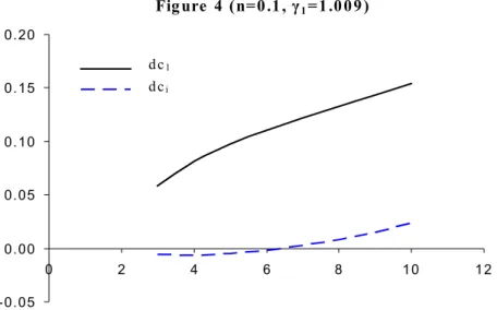
Figure 4 follows through on this logic. We illustrate the welfare gains as a function of the number of countries,N, assuming equal country size, so that n= 1/N, using the baseline estimates for all other parameters. From the discussion above, we know that peripheral countries do not benefit at all if there is zero discounting, zero money growth, and N = 3.

11_{Note however that the counterfactual involved is not necessarily equivalent to a policy change, since}

the move from STE to VCE is not chosen by governments. In addition, we could argue that the STE allocation is not a historically observed outcome.

Thus, for N = 3, β < 1, and γ1 > 1, peripheral countries are worse off in a VCE. Thus,

in the baseline calibration, peripheral countries only gain from a VCE if N is above a critical level. For Figure 3, a vehicle country is beneficial to the peripheral countries only for N _≥ 6. But then as N rises above this, the welfare gains rise exponentially. While the efficiency gains from a vehicle currency are clearly higher for large N, an interesting feature of these gains is that for peripheral countries, the gains may not be monotonic in

N. Figure 4 illustrates this effect by showing the gains to VCE for a higher rate of country 1 inflation. In this case, country 1 gains are higher, not surprisingly. But also, for smallN, peripheral country gains may befallinginN initially. The intuition for this negative effect of N is that increasing the number of countries makes each country more open, because it consumes approximately 1₋1/N of total goods as imports. This means that in the VCE, it is more exposed to the inflation tax of country 1, while in the STE this has no effect. Hence, beginning at N = 3, an increase in N may reduce welfare for a peripheral country initially, relative to STE. But asN rises further, the benefits of reduced transactions costs take over, and the gains are increasing in N.

Note that while the VCE offers welfare gains for the world economy, the distribution of gains depends on the money growth rate of country 1. Figure 5 illustrates the gains in the baseline calibration, except setting γ1 = 1. In this case the gain to each peripheral

country is larger, and the gain to the VC country falls from 15 percent to 9 percent. Thus 6 percent of the welfare gain in the baseline case is due to the monetary policy followed by the VC. Note that the overall worldwelfare gain is relatively independent of γ1. The gain

for the VC country is offset closely by the losses to peripheral countries.

How high can γ1 increase before it eliminates the gains for the peripheral countries?

This will depend upon both N and n. For a large number of countries, and a VC country which is large relative to others, there are still gains to a vehicle currency even for high rates of VC money growth. Figure 6 shows the gains to peripheral countries, for various levels of γ1. When n = 0.1 (VC country equal size), peripheral gains from the VC are

eliminated at γ1 = 1.036. But if n = 0.2, there are still gains to peripheral countries

for γ1 < 1.044. Thus, VC country inflation rates can be very high before eliminating the

welfare gains to a vehicle currency.

Nevertheless, the above result raises questions about the degree to which the VCE itself is sustainable in face of high centre country money growth. Moreover, in assessing the benefits to a vehicle currency, there is a clear trade-off between the rate of inflation in the VC country and the size of the VC country. In the next section, we explore the question of sustainability of a vehicle currency, and show how it relates to this trade-off.

5. Robustness of the Vehicle Currency Equilibrium

We have shown that there may be large welfare gains to a vehicle currency equilibrium. But we did not show how a vehicle currency arises, or which currency will play the role of a vehicle currency. Because of the trading technology and the existence of fixed costs, there are many equilibria in the model. Such multiplicity is inevitable when there arefixed costs of organizing the currency exchange. If some bilateral markets are not open, then