University of Ljubljana
Faculty of Computer and Information Science
Luka Lan Gabriel
Ear detection with convolutional
neural networks
BACHELOR’S THESIS
UNDERGRADUATE UNIVERSITY STUDY PROGRAMME COMPUTER AND INFORMATION SCIENCE
Mentor
: assoc. prof. dr. Peter Peer
Univerza v Ljubljani
Fakulteta za raˇ
cunalniˇ
stvo in informatiko
Luka Lan Gabriel
Detekcija uhljev s konvolucijskimi
nevronskimi mreˇ
zami
DIPLOMSKO DELO
UNIVERZITETNI ˇSTUDIJSKI PROGRAM PRVE STOPNJE
RA ˇCUNALNIˇSTVO IN INFORMATIKA
Mentor
: izr. prof. dr. Peter Peer
Copyright. The results of this Bachelor’s Thesis are the intellectual property of the author and the Faculty of Computer and Information Science, Uni-versity of Ljubljana. Publication or usage of the results of this Bachelor’s Thesis requires written consent of the author, the Faculty of Computer and Information Science, and the supervisor.
Faculty of Computer and Information Science issues the following thesis: Ear detection with convolutional neural networks
Topic of the thesis:
In recent years ears became a promising biometric modality. The first step in a biometric system is detection. Present the field of automatic ear detec-tion in images. Solve the ear detecdetec-tion problem with convoludetec-tional neural networks. Compare obtained results with other methods.
Fakulteta za raˇcunalniˇstvo in informatiko izdaja naslednjo nalogo: Detekcija uhljev s konvolucijskimi nevronskimi mreˇzami
Tematika naloge:
Uhlji so se izkazali kot dobra biometriˇcna modalnost. Prvi korak v biome-triˇcnem sistemu je detekcija. Preuˇcite in predstavite podroˇcje samodejne detekcije uhljev na slikah. S pomoˇcjo konvolucijskih nevronskih mreˇz reˇsite problem detekcije uhljev. Dobljene rezultate primerjajte z ostalimi meto-dami.
Za pomoˇc pri izdelavi diplomske naloge se iskreno zahvaljujem mentorju izr. prof. dr. Petru Peeru ter asistentu ˇZigu Emerˇsiˇcu.
Prav tako se zahvaljujem celotni ekipi Laboratorija za raˇcunalniˇski vid za prijetno druˇzbo v ˇcasu, ki sem ga tam preˇzivel.
Contents
Abstract Povzetek
Razˇsirjeni povzetek
1 Introduction 1
1.1 Motivation . . . 2
1.2 Object Detection . . . 2
1.3 Structure of the Thesis . . . 3
2 Related Work 5 3 Method 7 3.1 Artificial Neural Networks . . . 7
3.2 Convolutional Neural Networks . . . 11
3.3 Network Architecture . . . 13
3.4 Types of Layers Used in Our Model . . . 16
3.5 Training Datasets . . . 20
3.6 Training . . . 23
4 Results and Discussion 27 4.1 Comparison to Similar Approaches . . . 31
5 Conclusions 37
Abstract
Title: Ear detection with convolutional neural networks
Object detection is still considered a difficult task in the field of computer vision. Specifically, earlobe detection has become a popular application as the interest in human identification using earlobe biometry has increased. So far earlobe detection problem has been solved using a combination of skin detection, edge detection, segmentation by fusion of histogram-based k-means, and template matching algorithms. In this work we present a method of earlobe detection without template matching by using a convolutional neural network, performing image segmentation. With this method, which is invariant to angle at which the photo was taken, earlobe shape, skin color, illumination, occlusions, and earlobe accessories, we were able to accurately detect the area of the image, where an earlobe is present. Moreover, detection time was significantly improved when compared to other methods for solving the same task. We expect our method to be used in Annotated Web Ears Toolbox.
Keywords: computer vision, segmentation, convolutional neural networks, earlobe detection.
Povzetek
Naslov: Detekcija uhljev s konvolucijskimi nevronskimi mreˇzami
Zaznavanje objektov na slikah je ˇse zmeraj zahteven problem na podroˇcju raˇcunalniˇskega vida. Zaznavanje uhljev je v zadnjih letih postala popularna aplikacija zaznavanja objektov, z vedno veˇcjim zanimanjem za identifikacijo ljudi glede na biometrijo uhlja. Kolikor vemo, se je problem zaznavanja uhljev do zdaj reˇseval s kombinacijami zaznavanja koˇze, zaznavanja robov, his-togramov in algoritmi ujemanja predloge. V tem delu predstavimo metodo za detekcijo uhljev brez ujemanja predloge, z uporabo konvolucijske nevronske mreˇze, ki opravlja segmentacijo. S to metodo, ki je invariantna na kot, pod katerim je slika zajeta, obliko uhlja, barvo koˇze, osvetljitev, delno prekrivanje in dodatke na uhljih, smo uspeli natanˇcno zaznati obmoˇcje slike, kjer se uhelj nahaja. Nadalje, ˇcas, potreben za zaznavo, se je zelo izboljˇsal v primerjavi z ostalimi metodami za reˇsevanje enakega problema. Predvidevamo, da bo naˇsa metoda uporabljena v orodju Annotated Web Ears Toolbox.
Kljuˇcne besede: raˇcunalniˇski vid, segmentacija, konvolucijske nevronske mreˇze, detekcija uhljev.
Razˇ
sirjeni povzetek
Zaznavanje objektov na slikah je za ljudi preprosta naloga, ki jo opravl-jamo praktiˇcno podzavestno. Za raˇcunalnike pa ista naloga predstavlja velik problem, saj se ti ne morejo zavedati vsebine slik v svojih pomnilnikih. Pri zaznavanju objektov gre za proces zaznave pojavitve primerkov doloˇcenega razreda iz resniˇcnega sveta v digitalnih slikah. Znane aplikacije zaznave objektov vkljuˇcujejo zaznavo ˇcloveˇskih obrazov, peˇscev, vozil in promet-nih znakov. Objekte pa lahko zaznavamo tudi v videih, kar nam omogoˇca izdelavo avtonomnih vozil ter varnostni nadzor v realnem ˇcasu. Na po-droˇcju raˇcunalniˇskega vida je zaznavanje objektov trenutno zanimiv problem, katerega se s pomoˇcjo razliˇcnih metod tudi uspeˇsno reˇsuje. Med najveˇckrat uporabljene metode spadajo ekstrakcija znaˇcilk, klasifikacija z deskriptorjem znaˇcilk in metoda iskanja ujemanja s predlogo.
S poveˇcevanjem zanimanja po identifikaciji ljudi glede na biometrijo uˇseˇsa, se je pojavila tudi aplikacija zaznavanja objektov na zaznavanje ˇcloveˇskih uhljev. Uhlji se lahko pojavijo v razliˇcnih oblikah, razliˇcnih barvah koˇze, na njih so lahko dodatki (npr. uhani, sluˇsalke, sluˇsni aparat), njihovo vidnost lahko ovirajo ostali objekti (npr. lasje, pokrivala). Prav tako so lahko slike zajete pod razliˇcnimi pogoji, kot je kot, pod katerim je uhelj fotografiran in osvetljenost zajete slike. Vse naˇstete lastnosti oteˇzujejo detekcijo uhlja na slikah.
Reˇsitve v veˇcini za detekcijo uhlja uporabljajo stopnje ujemanja iskanega uhlja z roˇcno ustvarjeno predlogo. Ta se trudi zajeti ˇcimveˇc razliˇcnih ob-lik uhljev s kreiranjem idealiziranega oziroma povpreˇcnega uhlja. Nadalje,
razvita je bila metoda, kjer v obzir vzamejo tudi dejstvo, da so uhlji razliˇcnih velikosti. Tako so uvedli predlogo, katere velikost se spreminja glede na ve-likost zaznane glave. Ker obe metodi delujeta na principu detekcije robov, lahko pride do teˇzav, kadar uhelj delno prekrivajo ovire, s tem do ujemanja s predlogo ne pride. Razvita je bila tudi metoda, ki obide moˇznost delnega prekrivanja na naˇcin, da pri zaznavi ne iˇsˇce celotnega uhlje, ampak samo najbolj notranji del. Celoten uhelj nato, glede na znano pozicijo notranjega dela, zazna na podlagi bioloˇskih karakteristik ˇcloveˇskih uljev (npr. razmerje med viˇsino in ˇsirino). Z navedenimi metodami pa ˇse zmeraj ne reˇsimo prob-lema s fotografijami uhljev, ki so bile zajete z razliˇcnih kotov, saj se v takih primerih predloga ne more uspeˇsno prilagajati. Zato predlagamo metodo za segmentacijo uhljev na osnovi konvolucijske nevronske mreˇze.
Konvolucijske nevronske mreˇze predstavljajo razliˇciˇco umetnih nevron-skih mreˇz, katerih aplikacije zajemajo tudi razpoznavanje signalov, slik ter obdelavo naravnega jezika. Mreˇze so sestavljene iz veˇc plasti, ene vhodne, ene ali veˇc skritih in ene izhodne plasti. Na vhodni plasti podamo vhodne po-datke, sliko, ki jo s pomoˇcjo razliˇcnih vrst skritih plasti obdelamo. Na vsaki izmed skritih plasti se izraˇcunajo doloˇcene znaˇcilke. Na zadnji plasti iz pri-dobljenih znaˇcilk razberemo podatke o sliki, obiˇcajno verjetnosti, da se objekt doloˇcenega razreda na sliki pojavi. V naˇsi reˇsitvi je bila uporabljena knjiˇznica Caffe, odprtokodno ogrodje za globoko uˇcenje. Osnova naˇse arhitekture je arhitektura SegNet, ki v osnovi izvaja segmentacijo slik mestnih ulic in zaz-nane objekte razvrˇsˇca v 12 razredov. Osnovna arhitektura je bila prilagojena tako, da zaznava dva razreda: uhlje in ozadje – vse ostalo, kar ni uhelj. Vsako nevronsko mreˇzo pa je pred uporabo za reˇsevanje naloge potrebno tudi nauˇciti na uˇcni mnoˇzici.
Uporabljene uˇcne mnoˇzice so bile zgrajene s slikami iz baze Annotated Web Ears (AWE), pol-avtomatsko pridobljene mnoˇzice 1.000 anotiranih uh-ljev, ki pripadajo 100 razliˇcnim subjektom. Namesto obrezanih in anoti-ranih slik uhljev, smo morali uporabiti originalne, neobrezane slike in jih ponovno anotirati za potrebo naloge – segmentacijo. Anotacija uhljev je bila
opravljena na dva naˇcina. Pri prvem naˇcinu smo uhlje anotirali avtomatsko. Izraˇcunana je bila korelacija med neobrezano in pripadajoˇco obrezano sliko uhlja. Pozicija uhlja je bila najdena tam, kjer je bila izraˇcunana najviˇsja vrednost korelacije. Na najdeni poziciji je bil narisan pravokotnik dimen-zij obrezane slike uhlja. To je predstavljalo zelo grobo oznaˇcene slike in zaradi potrebe po bolj natanˇcno oznaˇcenih slikah (predvsem pri testiranju natanˇcnosti segmentacije), so bile slike tudi roˇcno oznaˇcene na osnovi po-sameznih slikovnih elementov. Zaradi majhnega ˇstevila uˇcnih primerov je bila uˇcna mnoˇzica tudi obogatena. Izvedene so bile tri vrste obogatitev: horizontalni zasuk, nakljuˇcno obrezovanje in kombinacija obojega.
Uˇcenje mreˇze smo izvajali na grafiˇcni procesni enoti, saj je njena zmoglji-vost pri uˇcenju mreˇz veliko viˇsja od zmogljivosti centralne procesne enote, zaradi zmoˇznosti paralelnega raˇcunanja. Pred zaˇcetkom uˇcenja smo celotno uˇcno mnoˇzico skopirali v grafiˇcni pomnilnik in s tem zmanjˇsali ˇcas, potreben za dostop do podatkov. Za 10.000 iteracij uˇcenja mreˇze smo potrebovali 64 minut. V tem ˇcasu sta vrednosti natanˇcnosti in izgube konvergirali k ˇzeljenim vrednostim. Vrednost natanˇcnosti, katera predstavlja odstotek pravilne klasi-fikacije posameznih slikovnih elementov v pripadajoˇce razrede, je konvergi-rala proti 100 in vrednost izgube, katera pove, kako nepravilni so v danem trenutku parametri nevronske mreˇze (na primer uteˇzi), je konvergirala proti 0.
Predlagana metoda je zmoˇzna zaznavanje uhljev v povpreˇcju opravljati z 98,69% natanˇcnostjo, kar pomeni, da na podani sliki pravilno klasificira 98,69% slikovnih elementov. Za segmentacijo ene slike metoda v povpreˇcju potrebuje 87,5ms kar pomeni, da lahko detekcijo opravljamo v realnem ˇcasu pri frekvenci 11 sliˇcic na sekundo. V primerjavi s sorodnimi deli, naˇsa metoda detekcijo opravlja z do 7% viˇsjo natanˇcnostjo v do 28 krat krajˇsem ˇcasu. S prilagajanjem strukture mreˇze, glede na nalogo, katero opravlja in veˇcjo mnoˇzico uˇcnih primerov, bi bilo mogoˇce delovanje mreˇze dodatno izboljˇsati.
Chapter 1
Introduction
Object detection is a task easily performed by humans. But the same task represents a much bigger problem to the computers. This holds true because of the fact that computers are not aware of the content of images they store in their memory. That is why object detection is at the moment still considered an interesting topic in the field of computer vision. Only recently has there been a breakthrough in tackling the mentioned problem. With the increased computing power and help of Convolutional Neural Networks (CNN) [16] more or less the same methods can be used to detect any kind of object as long as one is able to provide sufficient amount of images to train the network.
With the increase of interest in biometry of ears and human recognition by their earlobe, we decided to find a way to detect earlobes using CNNs. We wanted to provide a system, which is able to quickly and accurately locate an earlobe in an image regardless of its color, position, and shape. The method we decided to use was pixel-wise image segmentation using two classes: earlobe and everything else (background).
2 CHAPTER 1. INTRODUCTION
1.1
Motivation
This thesis, which belongs in the field of computer vision or more specifically object detection, is a part of a broader project by ˇZiga Emerˇsiˇc, Vitomir ˇ
Struc and Peter Peer [6]. The project addressees the identification of people by the biometry of their earlobe. In this thesis the detection of ears in images will be covered. This will help building a database of earlobes as well as detecting ears in an image in the process of human identification. Moreover a database of 1,000 annotated images will be built for the purpose of solving earlobe segmentation problems. The problem of earlobe detection will be solved using Convolutional Neural Networks (CNN) since it has (as far as we know) not yet been solved using this method. Annotation of earlobes for the database will be done manually. Binary masks will be created, where the marked areas will present an earlobe and the rest background. The images will be properly divided in the train and the test set and the created database will be used for training of the CNN as well as testing to obtain information about the accuracy of detection.
1.2
Object Detection
Object detection is a process of detecting instances of a certain class from the real world in digital images [2]. The task belongs to the field computer vision and image processing. Well known applications of object detection include face detection, pedestrian detection, vehicle detection and detection of road signs. Videos can also be processed for object detection, thus, allowing the technology to help create driverless cars by detecting objects on the road [1]. Another application alongside autonomous driving is real-time surveillance. Algorithms for object detection typically use feature extraction, classifica-tion with histograms of oriented gradients, template matching or learning algorithms [24], [26], [27]. The later is found in the rising method of object detection with the use of Convolutional Neural Networks.
1.3. STRUCTURE OF THE THESIS 3
1.3
Structure of the Thesis
First, we list and briefly describe the works that have already been done in the field of earlobe detection and mention the most common problems they face. Next, some theoretical background is presented about artificial neural networks and convolutional neural networks in particular. Also, the architecture of our model is described and its building blocks, layers, are further explained. Afterwards, different kinds of datasets, which were used to train the network, are explained, as well as the procedures of how they were obtained. The main points about the process of training the network are described next. Following, is the presentation of results with discussion and comparison to similar approaches. We conclude the thesis with identified problems we faced during our work and propose some improvements, which could better our results.
Chapter 2
Related Work
Earlobe detection is a challenging problem as earlobes appear in various shapes, sizes, and colors. Moreover, the images in which they appear may be of different illumination and the angles from which the images are taken may not always be ideal.
The problem of various shapes of an earlobe has been studied in many researches. The most straightforward approach is creating an idealized tem-plate [24], which aims to include most of the shapes earlobes appear in. But as earlobes are also of various sizes, a method with a resizing idealized tem-plate [26] seem as a more appropriate approach. Unfortunately, both of these methods rely on edge detection, which can be a problem if occlusions, such as earrings or hair covering the earlobe, appear in the image.
A method which tries to avoid this problem has been developed in [32]. As opposed to most other methods this one detects the inner part of the earlobe, which means light occlusions from earrings and hair are not a prob-lem anymore. By simply finding its center, some biological characteristics are taken into account to then detect the rest of the earlobe. But even with the use of this method an earlobe cannot always be detected if the image is taken from an angle, where the inner part is not visible.
Thus, a method invariant to illumination, pose, shape and occlusion has been proposed [27], providing satisfactory results. But as this method still
6 CHAPTER 2. RELATED WORK
uses a template for evaluating whether or not an earlobe is present within a region of interest, we believe the accuracy of detection could be improved.
We suggest a method that is based on convolutional neural networks. With this method we are able to make a pixel-wise classification (segmenta-tion) whether or not a part of the image belongs to an earlobe.
Chapter 3
Method
In this section we describe the suggested method based on convolutional neural networks. First, we describe what the used technologies are and how they work. Next, the architecture and the building blocks of the used model are further described. Also, we present the training datasets and how they were created. Finally we describe the process of training and briefly define some basic terms related to it.
3.1
Artificial Neural Networks
The first computational model for neural networks has been developed in 1943 by Warren McCulloch and Walter Pitts [18]. Their model was based on mathematics and algorithms called threshold logic. It served as the basis for neural networks method to split into two distinct approaches. One mimicking the biological processes in the brain and the other to develop an application of neural networks in the field of artificial intelligence.
Artificial neural networks (ANN) are a machine learning method inspired by a biological neural network. The methods try to mimic animals’ central nervous system, especially the brain. Similarly to a biological brain, neural networks are used to solve problems that depend on a large number of in-puts. An artificial neural network consists of a series of parallel nodes called
8 CHAPTER 3. METHOD
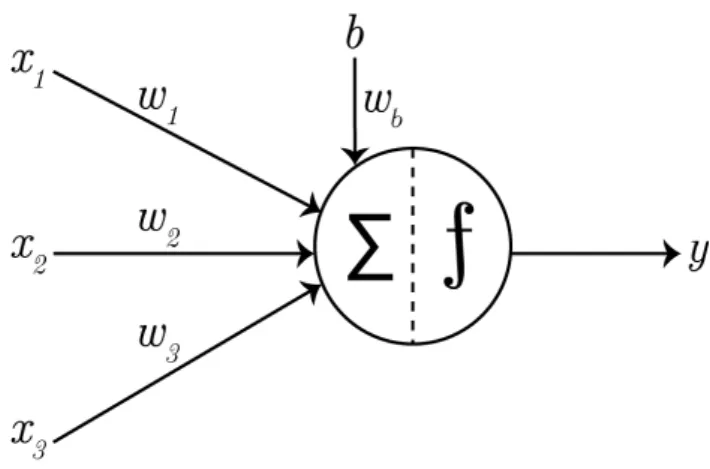
Figure 3.1: A simplified model of a neuron with x1,x2, andx3 as inputs,w1,
w2, and w3 as their corresponding weights, b presenting the bias, the circle
in the middle presents the neuron itself where the summer and activation function take place, and y presents the output of the neuron.
neurons, which are mathematical representation of simplified biological neu-rons. A mathematical model of a neuron (figure 3.1) consists of a number of weighted inputs, a weighted bias, a summer, an activation function, and an output [21]. The values of all inputs and the bias are weighted, summed, and if the sum is greater than a set threshold the activation function sends a signal from the output onto the input(s) of the next neuron.
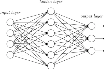
Neurons are grouped into layers that are interconnected. A neural net-work consists of an input layer, which sends the input data to the next layer, hidden layer(s), which can be used for any kind of processing of the input data, and output layer, which outputs the result of the given task. A specific structure of layers is normally called a model. An example model of an arti-ficial neural network is shown in figure 3.2. Neural networks are, like other machine learning methods, used to solve a variety of tasks, tasks otherwise hard to solve using rule-based programming.
To be able to solve given tasks, neural networks first need to be trained. To train a network you need a training dataset to learn from. The training dataset consists of raw data along with correct classifications, annotations,
3.1. ARTIFICIAL NEURAL NETWORKS 9
Figure 3.2: Example of a neural network with an input layer, one hidden layer and an output layer.
also called ground truths. These present the correct outputs of the network should the corresponding data be sent through the network for testing. A loss function is also present during training and tells how well or bad a model is able to predict the output after each iteration of learning. The goal of training a network is to find weights between neurons that minimize the loss function.
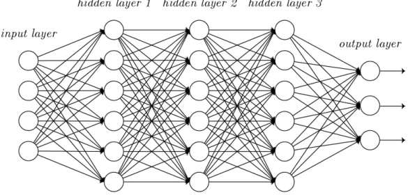
Complex neural networks consist of many layers that are connected with synapses (figure 3.3). Each synapse in an artificial neural network stores an adaptive weight. The adaptive weights represent the strengths between biological neurons and are constantly changing during training to produce the best results.
The described method can be compared to human vision. First, light waves hit the photoreceptors, which is an equivalent to data entering the input layer. Next the signal is processed through a series of biological systems and finally sent to the back of the brain, more specifically the V1 cortex [11]. V1 is the first stage of processing the visual information and still contains the information of the whole map of the visual field, resembling a hidden layer of
10 CHAPTER 3. METHOD
Figure 3.3: A more complex neural network with an input layer, three hidden layers, and an output layer. The image also shows how the outputs of one hidden layer are inputs of another.
an artificial neural network. The output of V1 is sent to subsequent cortical visual areas, where objects in the visual field are given meaning. Comparable to the output layer of the ANN.
However, the modern software implementations of ANNs are largely aban-doning the approach inspired by a biological brain. Instead they use a more practical approach that is based on statistics and signal processing [5].
The most common method for training ANNs is gradient descend with backpropagation. At every step of training, gradient of the loss function, according to all weights in the network, is calculated. In order to minimize the loss function an optimization method uses the calculated gradient to update the weights in the network accordingly. Since optimization requires differentiation, the activation functions in neurons need to be differentiable. In order to calculate the loss function, the desired output for every input needs to be known during training. The predicted output is compared to the desired output and the weights are then changed in the way that minimizes the difference between the two [4]. By doing this, the accuracy of predicted outputs rises.
3.2. CONVOLUTIONAL NEURAL NETWORKS 11
3.2
Convolutional Neural Networks
Convolutional neural networks, which are inspired by the animal visual cor-tex, are feed-forward neural networks, meaning the connections between all neurons are organized in such way that no cycle appears in the network. Similarly to ordinary neural networks, convolutional neural networks have an input, which is transformed through a series of hidden layers and at the end produces an output. They have a wide application range, such as image recognition or natural language processing [31].
When used for image recognition, convolutional neural networks consist of multiple layers of neuron clusters, which act as receptive fields. These clusters process the input image part by part and output a stack of features detected in the mentioned parts. The process is repeated at every such cluster and is used to tolerate translation, meaning the position of an object in an image is of no importance in order to still get recognized [12]. Local or global pooling layers are used to combine the outputs of neuron clusters.
The advantage of a convolutional neural network is the use of shared weights in convolutional layers. The same filter is used for each pixel within the same layer, which reduces memory needs and increases performance [15]. Another advantage is lack of dependence on prior knowledge of the studied object in the images and requirement for very little pre-processing. The network itself is responsible for learning filters in contrast to other algorithms that require human effort and knowledge to hand-engineer the filters.
Regular neural networks receive a single vector input, which is trans-formed through a series of hidden layers, where each neuron is fully con-nected. That is why regular neural networks do not scale well if working with images. CIFAR-10 [13] is a dataset of very small images. It consists of 60,000 colour images of size 32×32 pixels. In case a regular neural network would want to be trained and tested on the CIFAR-10 dataset, 32×32×3 (width, height, number of color channels, respectively), 3,072 weights per neuron would be needed, which is still manageable. But should the size of images increase, as in our case to 480×360, the number of weights per neuron
12 CHAPTER 3. METHOD
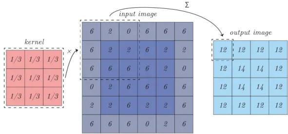
Figure 3.4: An example of convolution of an input with a 3×3 kernel.
reaches 518,400. As we would also want to use more than a single neuron, this would lead to a very high amount of weights needed and result in great memory requirement and decrease in performance.
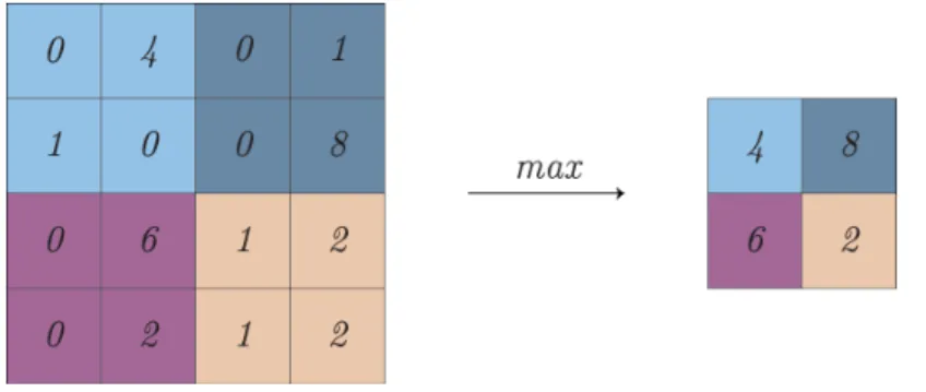
The convolutional neural networks assume that the input is always an image and because of this fact the architecture can be adjusted. In con-trast to regular neural networks, neurons of convolutional neural networks are arranged in three dimensions, width, height, and depth. In case of using CIFAR-10 dataset, the input layer of the network would be of a dimension 32×32×3. Moreover, the neurons are not fully connected. Instead, they are only connected to a small part of neurons from previous layer. For example, with a convolution filter (kernel) of the size 3×3, the size of the result of con-volution is 2 units smaller in height and 2 units smaller in width, compared to the size of the image before convolution, as shown in figure 3.4. Moreover, as convolution is an operation demanding a lot of computation, max pooling is typically used after convolution to reduce the size of data even further as well as reduce the amount of computation needed for any following convolutions, as shown in figure 3.5.
3.3. NETWORK ARCHITECTURE 13
Figure 3.5: An example of size reduction of a single depth slice by choosing the maximum values in 2×2 sized windows.
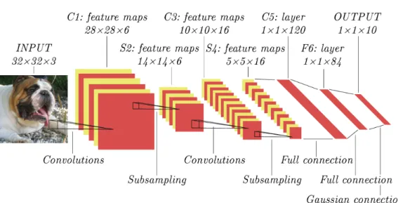
The last layer of a convolutional neural network is an output layer in shape of a vector. The dimensions of the vector are 1×1×n, where n equals the total number of classes present in a dataset. Classes from class scores vector, which are above a set threshold, are returned as results. In case of image segmentation the output layer is of the size w×h×n, where w and h are the width and height of the input image, respectively andn is the total number of classes present in a dataset. The end result corresponds to the class with maximum probability at each pixel [1]. An example convolutional neural network is shown in figure 3.6.
3.3
Network Architecture
In our work, the network was built using an opensource library, Caffe [10], a deep learning framework developed at the University of Berkley. The ben-efits of using Caffe are its simplicity and speed. The modularity of the library makes adding newly developed functions and types of layers easy. Caffe supports using GPUs to perform computation and allows the usage of CUDA, Nvidia’s parallel programming and computing platform, to reduce times needed to train networks.
SegNet [1] is a deep convolutional encoder-decoder architecture for robust semantic pixel-wise labeling. It consists of a sequence of nonlinear
process-14 CHAPTER 3. METHOD
Figure 3.6: A typical architecture of a convolutional neural network, here for image classification.
ing layers (encoders) and a corresponding set of decoders with a pixel-wise classifier. A single encoder consists of one or more convolutional layers, a batch normalization layer and a rectified linear units layer, followed by non-overlapping maxpooling and sub-sampling. A key feature of SegNet is the use of maxpooling in its decoders, which upsamples the low resolution fea-ture maps. With this feafea-ture high frequency details in segmented images are retained and the total number of parameters in decoders is reduced. The architecture can be trained by using stochastic gradient descend. The goal of a stochastic gradient descend is to find a minimum or maximum by iteration. In our case we are using it to find the minimum of the loss function.
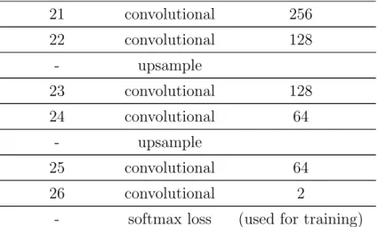
To be able to solve our task, a modification had to be done to SegNet’s last convolutional layer and the softmax loss layer. Number of outputs of the convolutional layer was changed to 2 (earlobe and background) and new class weights were calculated and applied to softmax loss layer to ensure a stable network training. A graphical representation of the architecture is shown in figure 3.7 and a tabular representation with layer numbers, types and numbers of outputs is shown in table 3.1.
3.3. NETWORK ARCHITECTURE 15
Layer Number Type of Layer Number of Outputs - data/input 480×360×3 1 convolutional 64 2 convolutional 64 - max pooling 3 convolutional 128 4 convolutional 128 - max pooling 5 convolutional 256 6 convolutional 256 7 convolutional 256 - max pooling 8 convolutional 512 9 convolutional 512 10 convolutional 512 - max pooling 11 convolutional 512 12 convolutional 512 13 convolutional 512 - max pooling - upsample 14 convolutional 512 15 convolutional 512 16 convolutional 512 - upsample 17 convolutional 512 18 convolutional 512 19 convolutional 256 - upsample 20 convolutional 256
16 CHAPTER 3. METHOD 21 convolutional 256 22 convolutional 128 - upsample 23 convolutional 128 24 convolutional 64 - upsample 25 convolutional 64 26 convolutional 2
- softmax loss (used for training)
Table 3.1: Tabular representation of the layers used in our architecture. A convolutional layer is always followed by a BN and a ReLU layer.
3.4
Types of Layers Used in Our Model
In the next sections, layers as building blocks of the used architecture are further described.
3.4.1
Data Layer
Data enters a network through data layers, which are placed at the begin-ning of a network. The data we feed our networks can enter from various sources. It can come from efficient databases such as levelDB, which is a fast key-value storage library written at Google or LMDB (Lightning Memory-mapped Database), a fast, memory-efficient database developed by Symas. Data can also come directly from memory or even from a disk when efficiency is not critical [16]. This way data can be stored either in HDF5, a file format for storing and managing data or in a common image format.
In our case, we are working with a small number of images, so efficiency is not critical. Thus, images in Portable Network Graphics (png) format are
3.4. TYPES OF LAYERS USED IN OUR MODEL 17
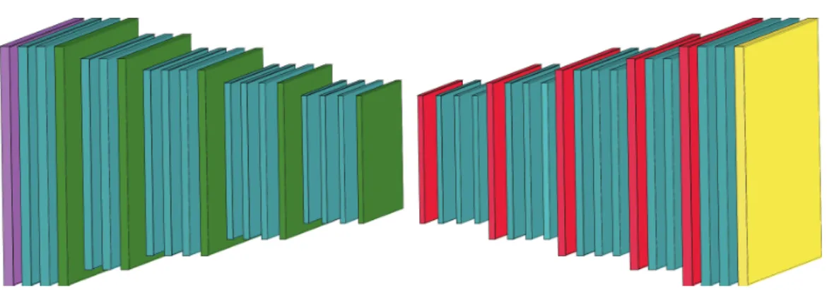
Figure 3.7: A graphical representation of the used architecture. The purple layer represents the input, data layer, each blue layer represents the sequence of a convolutional, a BN and a ReLU layer, green layers represent pooling layers, red layers represent upsample layers, and the yellow layer represents the output, softmax loss layer.
used.
Caffe also supports data augmentation in data layers [10], so image pre-processing like mean subtraction, scaling, random cropping and mirroring can be done automatically. But since our data has been augmented manually beforehand, additional augmentation has not been used. Another function from the data layer is shuffling. Data shuffling prevents the network from learning rules too specific to a series of similar images, which in a dataset tend to be placed one after another. In our case, we used data shuffling.
3.4.2
Convolutional Layer
The parameters of convolutional layers consist of a set of learnable filters [10]. Each filter is spatially small, but with horizontal and vertical shifting, it filters the whole input. Typical filter on the first convolutional layer of a network is for example a filter of the size 3×3×3 pixels (width, height, number of color channels, respectively). During the passing of the input to output, convolution is performed by all the filters of a convolutional layer. Convolution is a computation of dot products between the entries of the
18 CHAPTER 3. METHOD
filter and parts of the input volume of the size of the filter [3]. Dot product is computed at every position of the input volume to create a 2D activation map, a map of responses of the filter that we used at every position of the input. With iterations the network will help learn a filter to activate when they detect some type of visual feature. On the first convolutional layers of a network such features could be edges and convolutional layers on higher levels of the network could detect patterns. The entire set of filters produces corresponding activation maps. These maps are stacked on one another, similarly to color channels in images, to produce the output volumes.
3.4.3
Batch Normalisation Layer
A Batch Normalization (BN) layer allows the network to be trained at a higher learning rate, meaning the neural network may learn more quickly. With the use of BN layer the same accuracy can be achieved with 14 times fewer training steps [8]. When data flows through the network, weights and parameters adjust accordingly. But sometimes input data gets too big or too small and the weights and parameters may change drastically – problem referred to as internal covariate shift. Normalization, normalizing the data dimensions so that they are of approximately the same scale, is normally done as a part of pre-processing. Instead of one-time normalization at the beginning, the process is repeated at every BN layer.
3.4.4
Rectified Linear Units (ReLU) Layer
The Rectified Linear Units (ReLU) layer performs a threshold operation in the network, where the values less than zero are set to zero. Given an input valuex, ReLU computes the output y according to the equation 3.1.
y= x, if x >0 0, x≤0 (3.1)
3.4. TYPES OF LAYERS USED IN OUR MODEL 19
This means that the input and the output of a ReLU layer are the same layer. The values of the input layer are overridden by the values of the output of a ReLU layer.
3.4.5
Pooling Layer
Pooling layers are used to perform non-linear down-sampling – a decrease in dimensions of the data flowing through the network and so lowering the computational demands [7]. The input image is partitioned into a set of non-overlapping rectangles. Only the maximum value from each rectangle is preserved. By eliminating non-maximum values, much less computation is needed on the next layers of the network. The most commonly used filter size in a pooling layer is 2×2. This can be interpreted as dividing the input data into partitions of 2×2. Within each of the partitions only one among four values, the maximum, is preserved. These local maximum values are then tiled back together according to their position. With a single max-pooling layer the size of data at the output is only a quarter of that at the input, thus saving the network a lot of computation on the following layers.
3.4.6
Upsample Layer
Upsampling layer is, similarly as convolutional layer, a learnable layer [17]. It upsamples the feature maps from its input in a learnable way. The main idea is to use upsample layers to produce a feature map the size of the original image (as is on the data layer). A single upsample layer thus transforms a low resolution input into a higher resolution output. An upsample layer takes the learned filter from their pair convolutional layer and pastes the filter weighted by a scalar, the value from the input feature map, onto the output and repeats the process for all the values of the input feature map. Since some regions on the output overlap during the process, values at overlapping regions are simply added up.
20 CHAPTER 3. METHOD
3.4.7
Softmax Loss Layer
A softmax loss layer is implemented as the final layer of a convolutional neural network and is used for classification. This layer computes the multinomial logistic loss of the softmax of its input. Thus, it is conceptually identical to a softmax layer followed by a multinomial logistic loss layer [10]. Much like the binary logistic regression classifier, the softmax classifier is its generalization to multiple classes. Softmax function outputs a vector of real values between 0 and 1 that sums up to 1, representing the probabilities of all available classes being present in the feature map on its input [19]. The predicted probability distribution is then used as an input to the multinomial logistic loss function, which performs the one-of-many classification task and finally predicts the single class present in the input feature map.
3.5
Training Datasets
All the datasets were created with the help of Annotated Web Ears (AWE) dataset [6]. AWE is a dataset containing a total of 1,000 annotated images from 100 distinct subject, 10 images per subject. All images in AWE dataset were gathered from the web using a semi-automatic procedure and were labeled according to yaw, roll and pitch angles, ear occlusion, presence of accessories, ethnicity, gender and identity. The original, uncropped versions of these images, which are not part of the AWE dataset, were used and new annotations had to be created for the purpose of segmentation.
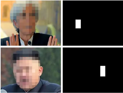
First, the original images and the cropped images from AWE dataset were gathered. Using an automatic procedure, the original images were annotated in a pixel-wise manner of where the ear is present and where it is not. The procedure used for this annotation was correlation between the original image and the cropped image. Where the correlation value was the highest, a rectangle of the size of the cropped image was drawn. Two examples of such annotation are shown in figure 3.8.
3.5. TRAINING DATASETS 21
Figure 3.8: Two examples and their corresponding ground truths obtained by using the automatic annotation using correlation. (In the images given here, faces were pixelated in order to guarantee anonymity.)
of a total of 582 images, 360 of which were used for training and 222 for testing. The reason for choosing these numbers is because they are the same as explained in SegNet usage procedure.
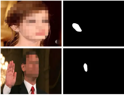
Next, a more detailed annotation has been done on the same number of images. While the images stayed the same, the earlobes in each picture were annotated manually. A precisely annotated dataset was needed to see how accurate the segmentation actually is as opposed to how many pixels inside a square are classified as an earlobe. With a total of 586 images, 367 of which were used for training and 219 for testing, the second dataset was created. Two examples of such annotation are shown in figure 3.9. The distribution of images in train and test sets is the same as in the first dataset.
Because neural networks produce better results with increasing time and number of images used for training [28], we decided to create a larger dataset. With a larger dataset we are able to prevent overfitting – creating a rule based classifier on a small amount of examples that is not necessarily true. Thus,
22 CHAPTER 3. METHOD
Figure 3.9: Two examples and their corresponding ground truths obtained by manual annotation. (In the images given here, faces were pixelated in order to guarantee anonymity.)
all images from the AWE dataset have been annotated manually. The third dataset consists of a total of 992 images, 744 (75% of the total number) of which were used for training and 248 (25% of the total number) for testing. A few images in all datasets were causing unknown errors during training. and were, therefore, removed. Upon further analysis it was found that the annotations of the images causing errors got corrupted during resizing and could not be used for training.
To investigate the statement that increasing the training dataset pro-duces better results even further, all of the above mentioned datasets were augmented. Data augmentation was done in three ways, horizontal flipping, random crops, and a combination of the two. Columns of pixels were flipped during horizontal flipping in such way that the first and the last column were swapped, the second and the penultimate were swapped, etc. For random crops, a pixel within the 20% of the height from the top and 20% of the width from the left was chosen at random. From the chosen pixel a rectangle was
3.6. TRAINING 23
drawn, the height of which was calculated by the equation 3.2: height = total image height−y value of the chosen pixel−
−random from 20% of total image height
(3.2) and width by the equation 3.3:
width = total image width−x value of the chosen pixel− −random from 20% of total image width.
(3.3) The image was cropped according to the selected rectangle. For the third aug-mentation the image was first horizontally flipped and then cropped. Identi-cal augmentations have been done to pairs of images and their corresponding annotations. With described augmentations applied to the three datasets, three new datasets were obtained with the numbers of images in the datasets quadrupled. The information about all datasets can be found in table 3.2.
3.6
Training
All of the neural networks have to be trained in order for them to perform their tasks. Our networks were trained on a GPU, since the performance using a GPU is much higher. We present the training process of the best performing network of our work.
Before the training, all images used in the network were resized to the resolution 480×360. This had to be done to reduce the needed graphical memory, since all images were first copied there to increase performance. A total of 2,128,896,016 bytes of graphical memory was needed for training on the images of dataset number 5. Another thing that had to be adjusted before the training was class weights on the softmax layer. These were calculated by the equation 3.4:
ac=
median frequency
frequency(c) , (3.4)
where frequency(c) is the number of pixels of class c divided by the total number of pixels in images where c is present and median frequency is the
24 CHAPTER 3. METHOD # Label Number of train images Number of test images Total number of images 1 Automatically annotated, small 360 222 582
2 Manually annotated, small 367 219 586 3 Manually annotated, full 744 248 992 4 Automatically annotated,
small, with augmentations 1,440 222 1,662 5 Manually annotated, small,
with augmentations 1,468 219 1,687 6 Manually annotated, full,
with augmentations 2,988 248 3,236 Table 3.2: Tabular representation of used datasets, described by their con-secutive number, applied label, number of images used for training, number of images used for testing and the total number of images.
3.6. TRAINING 25
median of these frequencies [1]. In our case, where only two classes are used, the median frequency is calculated as average of the two frequencies.
Learning rate was set to 0.0001 during training. Learning rate is a pa-rameter that controls how much the network’s weights will update in one training iteration. With a high learning rate, the loss function and accuracy change a lot during each iteration [29]. This can lead to instability and cause the loss function to diverge from its target value.
The momentum parameter, which helps prevent the training from con-verging to a local minimum, was set to 0.9. A momentum too high can cause radical avoiding of the local minima to destabilize the training process and a momentum too low can not reliably avoid them [9]. A well chosen momentum value can help the system converge faster.
The weight decay was set to 0.005. It is common to use weight decay while training, where every weight is multiplied by the weight decay value after each weight update, to prevent the weights from growing too large and, thus, causing instability [20]. Because of multiplication at every step, weight decay is exponential.
The training of the network took 64 minutes to complete 10,000 iteration and reach stable loss and accuracy values. Figure 3.10 shows the loss and accuracy values, which were collected in steps of 20 iterations throughout the course of the training process. We can see the loss converge towards 0 and accuracy towards 100%, which is the goal of the training.
The same architecture was used for training on all 6 datasets, only the class weights on the softmax loss layer had to be recalculated for each dataset.
26 CHAPTER 3. METHOD
Figure 3.10: Graphical representation of loss (red) and accuracy (blue) con-verging to their expected values during training. Values were obtained in steps of 20 learning iterations.
Chapter 4
Results and Discussion
The accuracy was measured by comparing the manually annotated images and the outputs of the network during testing. The pixels that are correctly classified as part of an earlobe are called true positives and the pixels that are correctly classified as everything but part of an earlobe are called true negatives. The equation used for calculating the accuracy of an image was (true positives + true negatives)/total number of pixels. Results can be seen in table 4.1 and figures 4.1, 4.2.
Among the 6 datasets on which we trained the network, the one that produced the best results was the dataset number 5 – the small, precisely annotated set with data augmentations consisting of 1,468 training images. With the network trained on the mentioned dataset we were able to achieve the average accuracy of 98.69% when testing on the corresponding test set, consisting of 219 images. With standard deviation of 0.80, we were also able to achieve the most reliable mean accuracy among all datasets.
Similarly, when the network was was trained on the dataset number 2 – the small, precisely annotated dataset consisting of 367 training images, we were able to achieve the average accuracy of 98.67% when testing on the corresponding test set, which was the same as for the training dataset number 5. The standard deviation of accuracies obtained with this dataset is 2.06, meaning the variation of accuracies is higher than in the aforementioned
28 CHAPTER 4. RESULTS AND DISCUSSION # Number of train images Number of test images Average accuracy (%) Standard deviation 1 360 222 98.60 1.47 2 367 219 98.67 2.06 3 744 248 98.29 0.99 4 1,440 222 97.71 2.09 5 1,468 219 98.69 0.80 6 2,988 248 97.49 1.76
Table 4.1: Table comparing the results between the six used datasets. From left to right the columns represent the enumeration of the training dataset, the number of images in the training dataset, the number of images in the test dataset, the average accuracy of segmentation prediction, and the standard deviation. Accuracies for all test images in each dataset were calculated, summed, and divided by the number of test images to obtain the average accuracies.
dataset, making the average accuracy value less reliable.
In contrast, when the network was trained on the dataset number 6 – the whole, precisely annotated set with data augmentation, the average ac-curacy was the lowest among all datasets used, 97.49%, when tested on its corresponding test set, consisting of 248 images. The standard deviation is 0.99, indicating the second most reliable average value.
The majority class accuracy of our data is 97.30%. This means that if all pixels were classified as everything but part of an earlobe, the average segmentation would be 97.30% accurate.
The hardware used during training and testing was a desktop PC with Intel(R) Core(TM) i7-6700K CPU with 32GB system memory and Nvidia GeForce GTX 980 Ti with 6GB of video memory running Ubuntu 14.04 LTS. In total six networks were trained and tested. The training of each network (10,000 iterations) lasted 64 minutes. The average test, segmentation pre-diction, was complete in 87.5 milliseconds.
29
Figure 4.1: Comparison between some ground truths, the predictions, and the differences between the two. Images in the left column represent ground truths, where white pixels represent the position of an earlobe, the ones in the middle are segmentation predictions, where white pixels represent the predicted position of an earlobe, and the ones in the right column show the difference between ground truth and the outcome of segmentation, where white pixels represent both false positives and false negatives.
30 CHAPTER 4. RESULTS AND DISCUSSION
Figure 4.2: Four sample images of the final earlobe segmentation results are shown. The images in the left column are original test images, the images in the middle represent segmentation predictions, and in the right column there are superimposed images composed of the original test image and the seg-mentation prediction. An example of a segseg-mentation prediction with some false positives can be seen in the last row, meaning some pixels were incor-rectly classified as earlobes. False positives are in our case better than false negatives, as broader areas in images can still be further processed in order to accurately localize earlobes. (In the images given here, faces were pixelated in order to guarantee anonymity.)
4.1. COMPARISON TO SIMILAR APPROACHES 31
Reference Dataset
Number of
test images Accuracy* (%) Time (s) Automated Ear Localization [27] UND-E 464 94.54 not mentioned Robust Localization of Ears [24] UND-J2 1776 99 not mentioned HEARD [32] UND-E 200 98 2.48 Ear Localization from Side Face Images [26] IT Kanpur ear database 150 95.2 not mentioned
This thesis AWE 219 98.69 0.087
Table 4.2: Table showing the results of our work and similar approaches. * Not all accuracies were calculated using the same equation — refer to explanations in section 4.1. The equations that calculate the percentage of correctly detected areas provide more detailed representations of accuracy than equations stating the rate of detection above a set threshold. The equation used in our work, where pixel-wise accuracy is calculated, provides the most detailed representation of accuracy.
4.1
Comparison to Similar Approaches
Six datasets mentioned above, were used to train our network. Among these, the dataset number 5 produced the best results, which will be used for com-parison to results obtained by similar approaches. A comcom-parison of figures is shown in table 4.2.
4.1.1
An Automated Ear Localization Technique
Ba-sed on Modified Hausdorff Distance
The authors of the paper [27] present a new scheme for automatic ear lo-calization. They are working with datasets of human profile images and
32 CHAPTER 4. RESULTS AND DISCUSSION
use template matching with modified Hausdorff distance. The benefit of the mentioned technique is that it does not depend on pixel intensity and that their template represents various ear shapes. Thus, this approach is invariant to illumination, pose, shape and occlusion in pictures taken from the side. The technique comprises of two parts, skin segmentation and edge detection. With the first part, they limit the detection of ears only to parts of the image containing skin. And as ear is a part of skin, non-skin regions can be skipped. The ear is then localized by computing the similarities of remaining relevant parts of the image and the ear template using modified Hausdorff distance. The detected ear is verified using normalized cross correlation technique. The accuracy of this technique was tested on two datasets, CVL face database [23] and UND-E database [22], on which accuracies of 91% and 94.54% were obtained respectively. Accuracy was calculated by the equation 4.1.
accuracy = number of true ear detection
number of test sample ×100 (4.1) The CVL and Collection E datasets contain mainly images of face profiles, which were taken under supervised conditions, and with the purpose of cre-ating a dataset. Moreover they are not as racially diverse as only Caucasians are found in the CVL dataset, and skin segmentation is know to be problem-atic with darker skins. Considering these factors, the mentioned datasets are less complex than the one we used in our work. No detection time is given by the authors.
4.1.2
Robust Localization of Ears by Feature Level
Fu-sion and Context Information
The ear detection algorithm, proposed in the paper [24] uses texture and depth images for localizing ears in both images of profiles of faces and im-ages taken with a different camera angle. Details on the ear surface and of edge images are used for determining the ear outline in an image. The proposed algorithm utilized the fact that the surface of the outer ear has
4.1. COMPARISON TO SIMILAR APPROACHES 33
a delicate structure with high local curvature. The algorithm consists of four steps: pre-processing, fusion of edges and shapes, computation of scores for ear candidates, and returning the ear region. In the pre-processing part edges and shapes are extracted from texture and depth image. With the use of depth images, mentioned parts are combined into full candidates for earlobe outlines. Next, a score is computed for every earlobe candidate by comparing it to an idealized ear outline. Lastly, the ear location is returned by the enclosing rectangle of the best ear candidate. The detection rate of this algorithm was found to be 99%. A detection was considered successful when the overlap O between the ground truth pixels G and the pixels in the detected region R is at least 50%. The overlapO was calculated by the equation 4.2.
O= 2|G
T
R|
|G|+|R| (4.2)
The databases used in the work are UND-J2 [25] and UND-NDOff-2007 [30]. UND-J2 consist only of profile views, while UND-NDOff-2007 serves as a more realistic dataset and consist of images taken at angles up to 90 de-grees off profile view. Even though the images are taken at various angles, they were still taken in supervised conditions with the purpose of creating a dataset as opposed to the complex dataset of images ”in the wild” we use in our work. No detection time is given by the authors.
4.1.3
HEARD: An Automatic Human EAR Detection
Technique
The method for ear detection HEARD [32] is based on three main features of a human ear: ear’s height to width ratio, ear’s area to perimeter ratio, and the fact that the ear’s outline is the most rounded outline on the side of a human’s face. The first stage of the proposed technique is image pre-processing, where the RGB values are converted to grayscale. Next, skin detection is applied, which marks the pixels of an image as either part of
34 CHAPTER 4. RESULTS AND DISCUSSION
skin or not. Thus, the output of this stage is an image of facial pixels only. In the next stage, edges above a certain length are detected and marked. To avoid occlusion caused by hair and earrings this ear localization method detects the inner part of the ear instead of the outer. When the inner part is localized the algorithm estimates the size and position of the ear according to the first feature about the human ear mentioned earlier. This method was able to detect 98% of ears in test photos. No information is given by the authors on how the accuracy was calculated. The method was tested on 200 samples chosen at random from the UND-E database [22], which consists of subject with various skin and hair color, with mild ear occlusions and taken on different backgrounds. Still, all the images were taken approximately 1.5 meters from the subjects and all images are of subjects’ left face profiles, making it a less complex database as used in our work. The detection time for a single image is 2.48 seconds.
4.1.4
Ear Localization from Side Face Images using
Distance Transform and Template Matching
Distance transform and template based technique is proposed in a paper [26] for automatic ear localization from side face images. First, skin segmentation is performed to eliminate parts of the image, which do not belong to a face. Skin regions are processed in separate stages. In the first stage an edge map is created, with edges that are not of a minimal required length and curvature removed. From this clean edge map a distance transform is obtained, which is used for the localization process. The ear template used in the localization process is resized according to the height and width of the face obtained from skin segmentation. Correlation between the resized template and distance transform is then calculated at every pixel. Locations, where the correlation value is above a certain threshold are considered probable locations of the ear. To validate, whether or not the location is actually that of an ear, the Euclidean distance between two sets of Zernike moments is calculated, first set belonging to the template and the second one to the detected ear. If the
4.1. COMPARISON TO SIMILAR APPROACHES 35
shortest calculated distance is below a precalculated threshold, detection of the ear is accepted. The accuracy of the described technique was found to be 95.2%. Accuracy was calculated by the equation 4.3.
accuracy = number of successful localizations
total sample size ×100 (4.3) For testing, IIT Kanpur ear database [26] was used. The database consists of side face images of 150 subjects, one image per subject, taken from the distance between 0.5 and 1 meter with light occlusions, making it a less complex database as used in our work. No detection time is given by the authors.
Chapter 5
Conclusions
Ear detection is a difficult problem that, in order to achieve good results on images taken under any condition, cannot be solved by template match-ing [14]. Various angles from which the photo was taken, earlobe shape, skin color, illumination, occlusions, and wearing accessories might present a problem for such a technique when detecting ears in photos taken “in the wild”.
With a diverse enough dataset we can overcome these problems by using convolutional neural networks to solve the task. In our work, even with the use of a small number of training images, this proved to be true as our method performed better than other methods for detecting ears known so far. Not only were we able to achieve a better accuracy, but also the time needed for detection was greatly reduced, even allowing real-time ear detection.
Still, there is room for improvements. Segmentation could have been better if the network structure was modified according to the task. Moreover, a much higher number of training images would be needed. The results might also improve with the use of cross-validation. Most of all, when annotating images, a clear rule would have to be made on which occurrences of ears should be detected and which should not, according to the angle and focus (blurrines).
Our results contradict the fact that accuracy should increase with a 37
38 CHAPTER 5. CONCLUSIONS
greater amount of training images. We suspect this occurred because in the first-third of AWE dataset, the images mostly contain a single occur-rence of an earlobe as opposed to the other two-thirds where more images contain multiple occurrences of earlobes, which lead to ambiguity. This con-sidered, the small, manually annotated dataset, with augmentations, pro-duced the highest average accuracy and the same set without augmentations produced second highest average accuracy, which complies with the fact ac-curacy should increase with a greater amount of training images. Moreover, the standard deviation of the augmented dataset was reduced.
In the end, an algorithm to crop the detected ears according to segmen-tation would have to be written, for our method to work as a fully functional module of AWE Toolbox. The method provides high accuracy and above all greatly reduces the detection times compared to all other methods mentioned in previous chapters.
Bibliography
[1] Vijay Badrinarayanan, Ankur Handa, and Roberto Cipolla. SegNet: A Deep Convolutional Encoder-Decoder Architecture for Robust Semantic Pixel-Wise Labelling. arXiv:1505.07293, 2015.
[2] Amruta Chavan, Dipali Bendale, Radha Shimpi, and Pradnya Vikhar. Object Detection and Recognition in Images. International Journal of Computing and Technology, 3(3):148–151, 2016.
[3] Mac A Cody. The wavelet packet transform, extending the wavelet transform. Dr. Dobb’s Journal, 19:44–46, 1994.
[4] David E. Rumelhart, Geoffrey E. Hinton, and Ronald J. Williams. Learning Representations by Back-propagating Errors.Nature, 323:533– 536, 1986.
[5] Daniel Dunea and Virgil Moise. Artificial Neural Networks as Support for Leaf Area Modelling in Crop Canopies. Proceedings of The 12th Wseas International Conference on Computers, pages 440–445, 2008. [6] ˇZiga Emerˇsiˇc, Vitomir ˇStruc, and Peter Peer. Ear Recognition: More
Than a Survey. Sent to Neurocomputing, 2016.
[7] Geoffrey E. Hinton and Nitish Srivastava and Alex Krizhevsky and Ilya Sutskever and Ruslan Salakhutdinov. Improving neural networks by pre-venting co-adaptation of feature detectors. arXiv, Computing Research Repository, 2012.
40 BIBLIOGRAPHY
[8] Sergey Ioffe and Christian Szegedy. Batch normalization: Accelerating deep network training by reducing internal covariate shift.arXiv preprint arXiv:1502.03167, 2015.
[9] Robert A Jacobs. Increased rates of convergence through learning rate adaptation. Neural networks, 1(4):295–307, 1988.
[10] Yangqing Jia, Evan Shelhamer, Jeff Donahue, Sergey Karayev, Jonathan Long, Ross Girshick, Sergio Guadarrama, and Trevor Dar-rell. Caffe: Convolutional Architecture for Fast Feature Embedding. arXiv:1408.5093, 2014.
[11] Eric Richard Kandel, James Harris Schwartz, Thomas M. Jessell, and Sarah Mack, editors.Principles of neural science. McGraw-Hill Medical, 2013.
[12] Keisuke Korekado, Takashi Morie, Osamu Nomura, Hiroshi Ando, Teppei Nakano, Masakazu Matsugu, and Atsushi Iwata. A convolutional neural network VLSI for image recognition using merged/mixed analog-digital architecture. In International Conference on Knowledge-Based and Intelligent Information and Engineering Systems, pages 169–176, 2003.
[13] Alex Krizhevsky and Geoffrey Hinton. Learning multiple layers of fea-tures from tiny images. Technical report, Canadian Institute For Ad-vance Research, 2009.
[14] Steve Lawrence, C. Lee Giles, Ah Chung Tsoi, and Andrew D. Back. Face recognition: A convolutional neural-network approach. IEEE transactions on neural networks, 8(1):98–113, 1997.
[15] Yann LeCun, Bernhard Boser, John S. Denker, Donnie Henderson, Richard E. Howard, Wayne Hubbard, and Lawrence D. Jackel. Back-propagation Applied to Handwritten Zip Code Recognition. Neural Computation, 1(4):541–551, 1989.
BIBLIOGRAPHY 41
[16] Yann LeCun, L´eeon Bottou, Yoshua Bengio, and Patrick Haffner. Gradient-Based Learning Applied to Document Recognition. Proceed-ings of the IEEE, 86(11):2278–2324, 1998.
[17] Jonathan Long, Evan Shelhamer, and Trevor Darrell. Fully Convolu-tional Networks for Semantic Segmentation.arXiv, Computing Research Repository, abs/1411.4038, 2014.
[18] Warren S. McCulloch and Walter Pitts. A logical calculus of the ideas immanent in nervous activity. The bulletin of mathematical biophysics, 5(4):115–133, 1943.
[19] Jonathan Milgram, Mohamed Cheriet, and Robert Sabourin. “One Against One” or “One Against All”: Which One is Better for Hand-writing Recognition with SVMs? In Tenth International Workshop on Frontiers in Handwriting Recognition, 2006.
[20] John Moody, Stephen Hanson, Anders Krogh, and John A. Hertz. A simple weight decay can improve generalization. Advances in neural information processing systems, 4:950–957, 1995.
[21] Michael A. Nielsen.Neural Networks and Deep Learning. Determination Press, 2015.
[22] University of Notre Dame. Profile Face Database, Collection E. Avail-able: http://www.nd.edu/cvrl/CVRL/DataSets.html (last access: Au-gust 3 2016).
[23] Peter Peer. CVL Face Database. Available: http://www.lrv.fri.uni-lj.si/facedb.html (last access: August 3 2016).
[24] Anika Pflug, Adrian Winterstein, and Christoph Busch. Robust lo-calization of ears by feature level fusion and context information. In International Conference on Biometrics, pages 1–8, 2013.
42 BIBLIOGRAPHY
[25] Ping Yan and Kevin Bowyer. Biometric Recognition Using 3D Ear Shape. Pattern Analysis and Machine Intelligence, 29:1297–1308, 2007. [26] Surya Prakash, Umarani Jayaraman, and Phalguni Gupta. Ear Local-ization from Side Face Images using Distance Transform and Template Matching. InWorkshops on Image Processing Theory, Tools and Appli-cations, pages 1–8, 2008.
[27] Partha Pratim Sarangi, Madhumita Panda, B. S. P Mishra, and Sachi-dananda Dehuri. An Automated Ear Localization Technique Based on Modified Hausdorff Distance. InInternational Conference on Computer Vision and Image Processing, pages 1–12, 2016.
[28] Dennis Shasha and Philippe Bonnet. Database Tuning: Principles, Ex-periments, and Troubleshooting Techniques (Part I). In ACM Interna-tional Conference on Management of Data, 2002.
[29] Boguslaw R. Szkuta, L. Augusto Sanabria, and Tharam S. Dillon. Elec-tricity price short-term forecasting using artificial neural networks.IEEE transactions on power systems, 14(3):851–857, 1999.
[30] Timothy Faltemier. Rotated Profile Signatures for Robust 3D Feature Detection. International Conference on Automatic Face Gesture Recog-nition, pages 1–7, 2008.
[31] Aaron van den Oord, Sander Dieleman, and Benjamin Schrauwen. Deep content-based music recommendation. In Advances in Neural Informa-tion Processing Systems 26, pages 2643–2651. Curran Associates, Inc., 2013.
[32] Nermin K. A. Wahab, Elsayed E. Hemayed, and Magda B. Fayek. HEARD: An automatic human EAR detection technique. In Interna-tional Conference on Engineering and Technology, pages 1–7, 2012.