HAL Id: hal-01715132
https://hal.archives-ouvertes.fr/hal-01715132v2
Submitted on 29 Oct 2019
HAL
is a multi-disciplinary open access
archive for the deposit and dissemination of
sci-entific research documents, whether they are
pub-lished or not. The documents may come from
L’archive ouverte pluridisciplinaire
HAL
, est
destinée au dépôt et à la diffusion de documents
scientifiques de niveau recherche, publiés ou non,
émanant des établissements d’enseignement et de
Averaging of density kernel estimators
O. Chernova, F. Lavancier, P. Rochet
To cite this version:
Averaging of density kernel estimators
O. Chernova, F. Lavancier and P. Rochet
November 4, 2019
Abstract
We study the theoretical properties of a linear combination of density kernel estimators obtained from different data-driven bandwidths. The average estimator is proved to be asymptotically as efficient as the oracle, with a control on the error term. The performances are tested numerically, with results that compare favorably to other existing procedures.
Keywords: Aggregation ; Bandwidth selection ; Non-parametric
estima-tion.
1
Introduction
Kernel estimation is an efficient and commonly used method to estimate a den-sity from a sample of independent identically distributed random variables. It relies on the convolution of the empirical measure with a functionK(the kernel), adjusted via a tuning parameterh(the bandwidth).
Several commonly used data-driven methods for bandwidth selection such as [Sil86] or [SJ91] have stood the test of time although none can be recog-nized as objectively best. In the past decades, aggregation for kernel density estimators has been investigated as an alternative to bandwidth selection. Meth-ods proposed in the literature include stacking ([SW99]), sequential processes
([Cat97, Yan00]) and minimization of quadratic ([RT07]) or Kullback-Leibler ([BDD+17]) criteria. In these papers, the initial estimators are assumed non-random, which is generally achieved by dividing the sample to separate training and validation.
The aim of the present article is to propose a new procedure to combine several competing density kernel estimators obtained from different, possibly data-driven, bandwidths. The method, in the spirit of model averaging, aims at minimizing the integrated square error of a linear combination of the kernel estimators. In this particular context, the first order asymptotic of the error is known up to a single parameter γ equal to the integrated squared second derivative of the density. The easily tractable error is precisely what makes kernel estimation a good candidate for averaging procedures, as we discuss in Section 2. Furthermore, the estimation ofγ can be made from the same data used to estimate the density so that no sample splitting is needed. The method is detailed in Section 3, where it is proved to be asymptotically as efficient as the best possible combination, referred to as the oracle. Our simulation study demonstrates that our method compares favorably to other existing procedures and confirms that sample splitting may lead to poorer results in this setting.
2
Some facts on kernel estimators
LetX1, ..., Xn be a sample of independent and identically distributed real
ran-dom variables with density f with respect to the Lebesgue measure. Given a kernelK:R→Rand a bandwidthh >0, the kernel estimator off is defined
as ˆfh(x) := (nh)−1P n i=1K h− 1(X i−x)
, x∈R. Henceforth, we assume that
Kis a bounded, symmetric around zero, density function onRsuch that
kKk2:=R K2(u)du <∞ and c K := R u2K(u)du <∞. (H K)
Concerningf, we assume it is twice continuously differentiable onRand
f,f0 andf00 are bounded and square integrable. (Hf)
Under (HK) and (Hf), [Hal82] showed that the Integrated Square Error
(ISE) of a kernel estimator ˆfhsatisfies
ISE( ˆfh) :=kfˆh−fk2= kKk2 nh +γ h4c2 K 4 +op 1 nh+h 4, (1) whereγ :=R
f00(x)2dx. In the typical case where (nh)−1 and h4 balance out,
meaning thath=O(n−1/5) andh6=o(n−1/5), or for shorthn−1/5, approx-imating ISE( ˆfh) is achieved from estimatingγ only. This result is technically
only valid for a deterministic bandwidth although in practice, most if not all common methods for bandwidth selection rely on some tuning parameters one has to calibrate from the data. Consequently, the bandwidth h is generally a data-driven approximation of a deterministic one h∗, hopefully sharing its asymptotic properties. The effect of this approximation can nevertheless be considered negligible if the integrated square errors are asymptotically equiva-lent, in the sense that
ISE( ˆfh)−ISE( ˆfh∗) ISE( ˆfh∗)
=op(1). (2)
We prove in the next proposition that this equivalence does generally hold true, implying that Hall’s result extends to data driven bandwidths. The set-ting encompasses most common data driven bandwidth selection procedures, as discussed after the proof. We moreover consider not only one but a collection ofk data-driven bandwidths h= (h1, ..., hk), in order to study the integrated
Gram matrix Σ with general term Σij=R fˆhi(x)−f(x)
ˆ
fhj(x)−f(x)
dx.
Proposition 2.1. Assume (HK), (Hf) and further that the kernel K has
compact support and is twice continuously differentiable. If there exists a de-terministic bandwidth h∗
i n−1/5 for all data-driven bandwidth hi satisfying
hi−h∗i =op(n−2/5), then
Σ =A+γB+op(n−4/5), (3)
whereAij =n1RK(u/hi)K(u/hj)duandBij:= 14h2ihj2c2K,i, j= 1, ..., k.
Proof. Following [HM87b], let ∆(h) = ISE( ˆfh) and consider the first-order
ex-pansion ∆(hi)−∆(h∗i) = (hi−h∗i)∆0(˜hi), for some ˜hibetweenhiandh∗i. From
Section 2 and Lemma 3.2 in [HM87b], we know that ∆0(˜hi) =Op(n−3/5).
Com-bined with the fact that ∆(h∗
i)Op(n−4/5), the conditionhi−h∗i =op(n−2/5)
implies ISE( ˆfhi)−ISE( ˆfh∗i)
/ISE( ˆfh∗
i) = op(1) for all i. Using the argu-ments of Theorem 2 in [Hal82], we get Σ =A∗+γB∗+op(n−4/5), where A∗
and B∗ are defined similarly as A and B with h∗i in place of hi. The map
(x, y)7→R
K(u/x)K(u/y)du is continuous for x, y > 0, which implies its uni-form continuity on every compact set in (0,+∞)2. Applying this function to
the sequences (x∗n, yn∗) = (n1/5h∗
i, n1/5h∗j), i6=j, which are bounded away from
zero, and (xn, yn) = (n1/5hi, n1/5hj), we deduce that n4/5(A−A∗) = op(1).
Similarly,n4/5(B−B∗) =op(1) yielding the result.
The most common bandwidth selection procedures do verify the condition
hi−h∗i =op(n−2/5) for some deterministic h∗ (see [JMS96]), making the
ap-proximation (3) available. For instance, Silverman’s rule of thumb approxi-mates the deterministic bandwidth h∗ = cmin{σ,iqr/1.34}n−1/5 where σ is
the standard deviation, iqr the inter-quartile range and c is either equal to 0.9 or 1.06, based on empirical considerations, see [Sil86]. The biased and
unbiased least-square cross-validation bandwidths discussed in [ST87, HM87b] and the plug-in approach of [SJ91] approximate the deterministic bandwidth
h∗ = kKk2/5(nc
Kγ)−1/5. The latter achieves a rate h/h∗−1 = Op(n−5/14)
that can be improved up to Op(n−1/2) if γ is estimated following [HSJM91].
Note finally that, as argued by several authors, a truncation argument allows to extend Proposition 2.1 to non compactly supported kernelsK, see e.g. [HM87c] or Remark 3.9 in [PM90].
3
The average estimator
Leth= (h1, ..., hk)>∈Rk+ be a collection of (possibly data-driven) bandwidths
and setˆf = ( ˆfh1, ...,fˆhk)
>. Following [LR16], we consider an estimator of f
expressed as a linear combination of the ˆfhi’s, ˆ fλ=λ>ˆf = k X i=1 λjfˆhi, (4)
where the weight vector λ = (λ1, ..., λk)> is constrained to sum up to one,
i.e. λ>1 = 1 for 1 = (1, ...,1)>. Under this normalizing constraint, the in-tegrated square error of ˆfλ has the simple expression ISE ˆfλ
= λ>Σλ. If Σ is invertible (which we shall assume throughout), the optimal weight vec-tor λ∗ minimizing the ISE under the constraint λ>1 = 1, is given by λ∗ =
1>Σ−11−1
Σ−11. The resulting average estimator ˆf∗ = λ∗>ˆf is called the oracle.
With all bandwidthshi of order n−1/5, we know from Proposition 2.1 that
Σ = A+γB+op(n−4/5). Because both A and B are known, approximating
Σ is reduced to estimating γ = R
f00(x)2dx. This problem has been tackled
in the literature, see for instance [HM87a, HSJM91, SJ91]. Hence, given an estimator ˆγofγ, one obtains an approximation of Σ byΣ =b A+ ˆγB. Replacing
Σ by its approximation Σ yields the average density estimator ˆb fAV = ˆfˆλ =
1>Σb−11 −1
1>Σb−1ˆf.
Theorem 3.1. Under the assumptions of Proposition 2.1, if Σ andΣb are
in-vertible andγˆ−γ=op(1), then
ISE ˆfAV = ISE( ˆf∗) 1 +op(1) . Proof. Write ISE( ˆfAV) = ˆλ>Σˆλ= ˆλ>Σˆbλ+ ˆλ> Σ−Σb ˆ λ. By construction, ˆλ>Σˆbλ ≤ λ∗>Σbλ∗ = λ∗>Σλ∗ +λ∗> Σb −Σ λ∗. Moreover, denoting by |||.||| the operator norm, |||A||| = sup||x||=1||Ax||, we have for all λ∈ Rk, |λ> Σ−Σb
λ| ≤ |||I−ΣΣb −1||| λ>Σλ,see the proof of Lemma A.1 in
[LR16]. Applying the above inequality to ˆλandλ∗, we get
1− |||I−ΣΣb −1|||
ISE( ˆfAV)≤ 1 +|||I−ΣΣb −1|||
ISE( ˆf∗) (5)
where we recall ISE( ˆf∗) =λ∗>Σλ∗. It remains to show |||I−ΣΣb −1|||=op(1).
By Proposition 2.1, Σ =A+γB+CwithA=Op(n−4/5),B=Op(n−4/5) and
C=op(n−4/5). Therefore b ΣΣ−1= (A+ ˆγB)Σ−1=I−CΣ−1+ (ˆγ−γ)BΣ−1 and sinceBΣ−1=O p(1), |||I−ΣΣb −1||| ≤ |||CΣ−1|||+|γˆ−γ|Op(1). (6)
The result follows from the fact thatCΣ−1=o
p(1) and ˆγ−γ=op(1).
fixed although the result remains valid if k = kn increases slowly with n. As
seen in the proof, the ISE of fˆAV approaches that of the oracle fˆ∗ provided
that|||I−ΣΣb −1|||=op(1). This can still be achieved ifkn increases sufficiently
slowly with n, e.g. logarithmically. In practice however, the numerical study shows that the results are less satisfactory with a too large number of initial estimators, due toΣbeing close to singular. For better performances, we suggest to use no more than four initial estimators, obtained from different methods, in order to reduce linear dependencies (see the discussion in Section 4).
One may be interested in setting additional constraints on the weights λi,
restrictingλ to a proper subset Λ⊂ {λ: λ>1= 1}. A typical example is to impose theλi’s to be non-negative, a framework usually referred to as convex
averaging. In fact, the same result as in Theorem 3.1 holds for any such subset Λ, using the corresponding oracle and average estimator, the proof being iden-tical. A reason for considering additional constraints onλis to aim for a more stable solution, which may be desirable in practice especially when working with small samples (see e.g. Table 1 in Section 4). However, since the oracle is nec-essarily worse (in term of integrated square error) for a proper subset Λ, the result lacks a theoretical justification for using a smaller set. Note that, on the contrary, the constraintλ>1= 1 is necessary for the equality ISE( ˆfλ) =λ>Σλ
to hold true.
The next proposition establishes a rate of convergence in the case where the bandwidthshi used to build the experts ˆfhi are deterministic and of the order
hi n−1/5. The additional assumption ˆγ−γ =op(n−2/5) is mild as the best
known convergence for an estimator ˆγ is ˆγ−γ = Op(n−1/2), see for instance
[HSJM91].
deter-ministic withhi n−1/5,ΣandΣb are invertible andˆγ−γ=op(n−2/5),
ISE( ˆfAV) = ISE( ˆf∗) +Op(n−6/5).
Proof. Under the assumptions, Theorem 2.1 applies with second order asymp-totic expansionC= Σ−A−γB=Op(n−6/5). In view of (5) and (6), the rate
of convergence for ISE( ˆfAV)−ISE( ˆf∗) follows from investigating|||CΣ−1|||and
|ˆγ−γ|. Here, |||CΣ−1|||=O
p(n−2/5) while |γˆ−γ|is negligible in comparison
by assumption.
The result of Proposition 3.3 improves on the residual termO(n−1) obtained
in [RT07] where the initial estimators, or experts, are built from a training sam-ple of sizentr, while the aggregation is performed on an independent validation
sample of size nva with n = ntr+nva. In fact, [RT07] show that
condition-ally to the training sample (making the experts built once and for all), their aggregation procedure reaches the minimax rateO(n−1
va), which is at best of the
orderO(n−1). In our setting, the rate of the residual term is improved due to
the initial kernel estimators contributing a factorOp(n−4/5).
4
Simulations
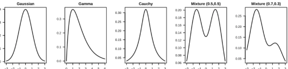
Based on a sample ofnindependent and identically distributed observations, we consider the estimation of the following density functions, depicted in Figure 4: the standard normal distributionN(0,1); the Gamma distribution with shape parameter 2 and scale parameter 1; the Cauchy distribution; the equiproba-ble mixture of N(−1.5,1) and N(1.5,1); and the mixture of N(−1.5,1) with probability 0.7 andN(1.5,1) with probability 0.3.
The initial kernel estimators are built with Gaussian kernel and data-driven bandwidthsnrd0(Silverman’s rule of thumb),nrd(its variation with
normaliz-−3 −2 −1 0 1 2 3 0.0 0.1 0.2 0.3 0.4 Gaussian dnor m(x) 0 1 2 3 4 5 6 0.0 0.1 0.2 0.3 Gamma −3 −2 −1 0 1 2 3 0.05 0.10 0.15 0.20 0.25 0.30 Cauchy −3 −2 −1 0 1 2 3 0.06 0.08 0.10 0.12 0.14 0.16 0.18 0.20 Mixture (0.5,0.5) −3 −2 −1 0 1 2 3 0.05 0.10 0.15 0.20 0.25 Mixture (0.7,0.3)
Figure 1: Densities functions considered in the numerical examples
ing constant 1.06), andSJ(the plug-in approach of Sheater and Jones), following the default choices in theRsoftware [R C17]. The least-square cross-validation bandwidths (ucvand bcvin R) are deliberately not included because they ap-proximate the same deterministic bandwidthh∗as Sheater and Jones’ method, which would result in an asymptotically degenerated (non-invertible) matrix Σ. This was confirmed by simulations (not displayed here), where the inclusion of these estimators did not improve the performances described below. The three kernel estimators are then combined by our method where ˆγ is estimated as in [HSJM91]. We also assess convex averaging where, in addition, the weights
λi are restricted to non-negative values. For the sake of comparison with
ex-isting techniques, we implement the linear and convex aggregation methods considered in [RT07] who also use a quadratic loss function. In their setting, the experts ˆfhi are computed from a training sample of half size, independent from the remaining validation sample on which the weights λi are estimated.
In the same spirit, we have also tested this splitting scheme for our average estimator, where ˆγ is estimated from the validation sample. For robustness, it is advised in [RT07] to average different aggregation estimators obtained over multiple sample splittings. We followed this recommendation and we considered 10 independent splittings into two samples of equal size.
n Law nrd nrd0 SJ . AV AVsplit RT AVconv RTconv 50 Norm 1936 1737 1902 . 1788 1698 2480 1844 2030 Gamma 1822 1903 1864 . 1897 2088 2685 1841 2173 Cauchy 1214 1289 1233 . 1292 1493 1778 1218 1452 Mix05 999 1043 1056 . 1239 1397 1393 1063 1164 Mix03 1086 1145 1155 . 1238 1401 1582 1159 1267 100 Norm 1057 957 1026 . 962 947 1325 998 1113 Gamma 1129 1239 1146 . 1153 1305 1615 1135 1376 Cauchy 748 848 756 . 775 906 1059 750 938 Mix05 634 699 677 . 796 922 888 705 772 Mix03 669 751 703 . 728 852 898 717 823 200 Norm 628 578 616 . 568 556 767 597 660 Gamma 701 795 705 . 701 772 944 696 839 Cauchy 462 540 454 . 452 531 613 454 585 Mix05 391 453 409 . 474 559 501 452 492 Mix03 398 470 406 . 395 467 486 412 510 500 Norm 310 286 299 . 276 274 346 292 321 Gamma 388 462 370 . 367 411 459 369 459 Cauchy 232 283 220 . 208 240 294 221 293 Mix05 210 253 209 . 223 258 227 240 264 Mix03 223 271 218 . 199 222 234 222 282 1000 Norm 183 171 177 . 163 163 196 174 191 Gamma 231 285 216 . 211 240 262 215 272 Cauchy 145 182 133 . 121 138 178 134 181 Mix05 126 158 120 . 120 138 120 134 159 Mix03 132 165 125 . 108 117 124 127 164 2000 Norm 111 104 106 . 99 98 113 105 114 Gamma 146 183 132 . 130 147 160 132 167 Cauchy 84 108 76 . 66 73 110 76 101 Mix05 79 100 73 . 68 74 68 79 95 Mix03 77 98 72 . 59 61 66 72 92
Table 1: Estimated MISE (based on 103replications) of the kernel estimators with bandwidths
nrd, nrd0orSJ(by default inR) and the combinations of these estimators by our method (AV), our method with sample splitting (AVsplit), the linear method in [RT07] (RT), our convex method (AVconv) and the convex method in [RT07] (RTconv).
The mean integrated square errors of the aforementioned estimators are summarized in Table 1, depending on the sample sizen. These errors are ap-proximated by the average over 103replications of the integrated square errors. It shows that our averaging procedure (AV in the table) outperforms every sin-gle initial kernel estimators when the sample size is large (n≥500) and the gain becomes significant whenn≥1000. On the contrary, our averaging procedure is inefficient for small sample sizes (n= 50), which is probably explained by a poor use of the asymptotic expansion of Σ in this case. In fact, the convex averaging procedure (AVconv in the table) seems preferable for smalln although it also
fails to achieve the same efficiency as the best estimator in the initial collection. A transition seems to occur for moderate sample sizes aroundn= 100, where the results of the average estimator are comparable to the best kernel estimator. In all cases, our averaging procedure outperforms the alternative aggregation method of [RT07]. Finally, according to the numerical results, a splitting scheme for our method (AVsplit in the table) is not to be recommended, suggesting that all the available data should be used both for the initial estimators and for ˆγ, which is in line with our theoretical findings.
References
[BDD+17] Cristina Butucea, Jean-Fran¸cois Delmas, Anne Dutfoy, Richard
Fis-cher, et al. Optimal exponential bounds for aggregation of estima-tors for the kullback-leibler loss. Electronic Journal of Statistics, 11(1):2258–2294, 2017.
[Cat97] Olivier Catoni. The mixture approach to universal model selection. Technical report, Ecole normale sup´erieure, 1997.
[Hal82] Peter Hall. Limit theorems for stochastic measures of the accuracy of density estimators. Stochastic Processes and their Applications, 13(1):11–25, 1982.
[HM87a] Peter Hall and James Stephen Marron. Estimation of inte-grated squared density derivatives. Statistics & Probability Letters, 6(2):109–115, 1987.
[HM87b] Peter Hall and James Stephen Marron. Extent to which least-squares cross-validation minimises integrated square error in non-parametric density estimation. Probability Theory and Related Fields, 74(4):567–581, 1987.
[HM87c] Peter Hall and JS Marron. On the amount of noise inherent in bandwidth selection for a kernel density estimator. The Annals of Statistics, pages 163–181, 1987.
[HSJM91] Peter Hall, Simon J Sheather, MC Jones, and James Stephen Mar-ron. On optimal data-based bandwidth selection in kernel density estimation. Biometrika, 78(2):263–269, 1991.
[JMS96] M Chris Jones, James S Marron, and Simon J Sheather. A brief survey of bandwidth selection for density estimation. Journal of the American Statistical Association, 91(433):401–407, 1996.
[LR16] Fr´ed´eric Lavancier and Paul Rochet. A general procedure to combine estimators. Computational Statistics & Data Analysis, 94:175–192, 2016.
[PM90] Byeong U Park and James S Marron. Comparison of data-driven bandwidth selectors. Journal of the American Statistical Associa-tion, 85(409):66–72, 1990.
[R C17] R Core Team.R: A Language and Environment for Statistical Com-puting. R Foundation for Statistical Computing, Vienna, Austria, 2017.
[RT07] Ph. Rigollet and A.B. Tsybakov. Linear and convex aggregation of density estimators. Mathematical Methods of Statistics, 16(3):260– 280, 2007.
[Sil86] B. W. Silverman.Density estimation for statistics and data analysis. Monographs on Statistics and Applied Probability. Chapman & Hall, London, 1986.
[SJ91] Simon J. Sheather and Michael C. Jones. A reliable data-based bandwidth selection method for kernel density estimation.Journal of the Royal Statistical Society. Series B (Methodological), 53(3):683– 690, 1991.
[ST87] David W Scott and George R Terrell. Biased and unbiased cross-validation in density estimation. Journal of the american Statistical association, 82(400):1131–1146, 1987.
[SW99] Padhraic Smyth and David Wolpert. Linearly combining density estimators via stacking. Machine Learning, 36(1):59–83, 1999. [Yan00] Yuhong Yang. Mixing strategies for density estimation. Ann.