Multi-Label Answer Aggregation for Crowdsourcing

Multi-Label Answer Aggregation for Crowdsourcing

Nguyen Thanh Tam

#

, Huynh Huu Viet

*

, Nguyen Quoc Viet Hung

*

,

Matthias Weidlich

†

, Hongzhi Yin

*

, Xiaofang Zhou

* #

École Polytechnique Fédérale de Lausanne *The University of Queensland †Humboldt-Universität zu Berlin

ABSTRACT

Crowdsourcing has been widely established as a means to enable human computation at large scale, in particular for tasks that re-quire manual labelling of large sets of data items. Answers ob-tained from heterogeneous crowd workers are aggregated to obtain a robust result. However, existing methods for answer aggregation assume that answers are given as a single label per item. Hence, these methods are ineffective for common multi-labelling problems such as image tagging and document annotation, where items are assigned sets of labels. In this paper, we propose a novel Bayesian nonparametric model for multi-label answer aggregation. It enables us to predict labels for non-grounded items, while taking into ac-count dependencies between the labels in different answer sets. We also show how this model is instantiated for incremental learning, incorporating new answers from crowd workers as they arrive. An evaluation of our method using a number of large-scale, real-world crowdsourcing datasets reveals that it consistently outperforms the state-of-the-art in answer aggregation in terms of precision, recall, and robustness against faulty workers and data sparsity.

1.

INTRODUCTION

Fuelled by the massive availability of Internet users, crowdsourc-ing has been widely established as a means for human computation at large-scale [24]. Tasks that are rather trivial for humans, but computationally expensive or even unsolvable for machines can be efficiently addressed by crowdsourcing. Specifically, crowdsourc-ing has been applied for such diverse applications as data acqui-sition [2], data integration [37], data mining [30], information ex-traction [12], and information retrieval [35]. Today, a large number of platforms, such as Amazon Mechanical Turk and CrowdFlower, facilitate the development of crowdsourcing applications.

Aggregation of Crowd Answers.Most crowdsourcing setups are based on questions (aka tasks) that, once posted to crowdsourcing platform, are answered by users (aka crowd workers) for financial rewards. Yet, each task is answered by multiple workers to accom-modate for their different levels of expertise and motivation [17]. Aggregation of answers obtained for a single task shall comple-ment individual errors, exploiting the ‘wisdom of the crowd’.

ACM ISBN 978-1-4503-2138-9.

DOI:10.1145/1235

Answer aggregation is challenging for several reasons. The wor-ker population may contain faulty worwor-kers (e.g., spammers) that give random answers, but are hard to identify before-hand in the ab-sence of detailed worker information. Furthermore, workers may be unintentionally biased by personal interest or systematic mis-understanding of the tasks [34]. Aggregation of answers is also complicated by limited mutual information between workers and tasks, e.g., some workers are assigned with too few tasks and vice-versa [36]. To overcome these challenges, various methods for au-tomatic answer aggregation have been proposed in the literature (see [15] for survey), including (i) non-iterative techniques which compute the aggregated answer as a linear combination of votes, and (ii) iterative techniques which leverage mutual reinforcing re-lations between workers and answers.

Multi-label Answer Aggregation. The above aggregation meth-ods have been developed for single-label tasks comprising of a set of labels and a set of items—a crowd worker is expected to assign a single label to each item. This assumption, however, does not hold for many crowdsourcing applications that received much at-tention recently, such as text categorization, image classification, and medical diagnosis [1, 6, 22]. These applications define multi-label tasks, where workers shall provide a set of multi-labels per item.

Despite the increased noise and bias due to the freedom to choose multiple labels per item, multi-label answer aggregation is inher-ently more complex than its single-label counterpart. First, the la-bels obtained as part of different answers are often correlated. For instance, in movie classification, movies about asuper-heroare of-ten associated with the genreaction[28]. Construction of a correct set of labels needs to deal with the exponential growth of combina-tions of labels and dependencies between them. Second, workers no longer either agree or disagree on the answer to a question, but consensus becomes partial. As a consequence, it becomes difficult to assess the reliability of workers since they may provide suppos-edly correct and incorrect labels at the same time.

Approach. In this paper, we propose a Bayesian nonparametric model in order to capture the distinct properties of multi-label an-swer aggregation. That is, co-occurrence dependencies between labels are represented by the notion of latent label clusters. This notion is motivated by the observation that items can be often be grouped together, if they share similar labels. Furthermore, par-tial consensus between workers is modelled by grouping together workers with similar answers. This enables us to construct an ag-gregated answer based on the consensus of groups of workers in-stead of consensus among individuals. The resulting model, called

Clustering-based Bayesian Combination of Multi-label Classifiers

(cBCMC), generalises models developed for single-label answer aggregation [20] and enables incremental learning using stochastic variational inference [13].

Contribution and Structure. Our contributions along with the structure of the paper can be summarized as follows:

Problem Setting(§2) We motivate the need for multi-label answers aggregation. We further elaborate on types of crowd workers, formalize the problem stetting, and outline requirements for so-lutions to the problem of multi-label answer aggregation. Fur-ther, we discuss the limitations of the state-of-the-art in using Bayesian nonparametric models for answer aggregation.

Novel Model for Multi-Label Answer Aggregation(§3) We present a generative model for multi-label answer aggregation, called

Clustering-based Bayesian Combination of Multi-label Classi-fiers (cBCMC). Specifically, we show how to perform model inference (finding the probability distribution of model param-eters given information on worker answers or true labels) and model instantiation (estimating item labels based on the given information and the inferred parameter distributions).

Methods for Incremental Computation(§4) To cope with the con-tinuous arrival of new answers in a crowdsourcing setting, we present methods for incremental computation. We show how model inference is facilitated by updating the model parameters based on new data instead of inferring a model from scratch.

Evaluation(§5) Experiments with real-world datasets highlight the effectiveness of the proposed cBCMC model, consistently out-performing the state-of-the-art in terms of precision, recall, and robustness against faulty workers. When using incremental learn-ing, we observe speed-ups of up to 17×in runtime, with only moderate reduction in label prediction accuracy.

Finally, §6 reviews related work, before §7 concludes the paper.

2.

PROBLEM SETTING

We first introduce a motivating example for multi-label answer aggregation and elaborate on challenges induced by different types of crowd workers. Then, we present a problem statement and dis-cuss requirements for potential solutions. Finally, we review the state-of-the-art in answer aggregation against these requirements.

2.1

Motivating Example

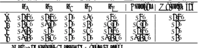
We consider an image tagging task, in which workers assign one or more labels to a picture. For simplicity, these labels are encoded by numbers from 1 to 5. Table 1 illustrates an exemplary crowd-sourcing result, in which five workers (u1-u5) provided their an-swers to four pictures (i1-i4). The correct, yet generally unknown, label assignment is shown in a separate column.

Table 1: Answers provided by five workers for four pictures u1 u2 u3 u4 u5 Correct Majority [4]

i1 {4,5} {4,5} {4} {1} {5} {5} {4,5}

i2 {2,3} {1,4} {4} {2} {3,4} {3,4} {4}

i3 {1,2} {4} {4} {3} {4,5} {4,5} {4}

i4 {1,2} {2,3} {4} {4} {1,2,3} {1,2,3} {2}

1: sky, 2: plane, 3: sun, 4: water, 5: tree

Answer aggregation computes, for each item, a joint answer based on the input provided by workers. A common method to derive an aggregated answer is majority voting [4], which considers all labels separately. If the ratio of ‘votes’ from workers for a label is larger than 0.5, the respective label is included in the aggregation result. Compared to the actually correct assignment, the result obtained in this case has two issues, though: (i) it is partially incorrect (e.g., la-bel 4 is not correct fori1), and (ii) partially incomplete (e.g. labels 1 and 3 shall also be assigned toi4).

These issues have two main causes. First, workers are considered equally, whereas it is well known that they have different charac-teristics. Previous studies [17] identified different types of crowd

workers: (1) Reliable workers have deep knowledge about specific domains and answer questions with high reliability; (2) Normal workers have general knowledge to give correct answers, but make mistakes occasionally; (3) Sloppy workers have little knowledge and often give wrong answers unintentionally; (4) Uniform spam-mers intentionally give the same answer for all questions; (5) Ran-dom spammers give ranRan-dom answers for all questions. For binary classification tasks, these types can be described by the two-coin model [39]. As illustrated in Fig. 1, it assesses worker quality in terms of sensitivity (the proportion of positives that are correctly classified) and specificity (the proportion of negatives that are cor-rectly classified). 0 0.2 0.4 0.6 0.8 1 0 0.2 0.4 0.6 0.8 1 Sensitivity (true positive)

Specificity (true negative) Crowd Simulation 15 Uniform Spammer Reliable Worker Normal Worker Uniform Spammer Sloppy Worker

Figure 1: Characterization of worker types

In the above example,u3 is a uniform spammer, assigning the same labels to all pictures. Yet, these answers are reflected in ag-gregated result. Removingu3, for instance, yields the correct result for picturei1. Workeru4is a random spammer, whereas the re-maining workers can be classified as truthful (u5) or normal (u1 andu3). In practice, different worker types are frequently encoun-tered. A recent study [39] reported on a population consisting of 38% spammers, 18% sloppy, 16% normal, and 27% reliable work-ers for a binary classification task.

A second cause for the issues observed in the example is the neglect of dependencies between labels. For instance, label 2 often co-occurs with labels 3 and 1. Such correlation can be useful in the aggregation. If we also include label 1 and label 3 whenever label 2 has been assigned, for instance, the obtained result would be correct for picturei4when using majority voting.

2.2

Problem Statement

We capture the setting of multi-label answer aggregation by a set of workers

U

, identified by their indices,

U

,{1, . . . ,U}that pro-vide answers for a set of items

N

, also identified by their indices,

N

,{1, . . . ,I}.

Z

,{1, . . . ,C}is the set of all possible labels for these items. Each answer by a crowd worker is a subset of

Z

. For-mally, answers are modelled as anI×U answer matrix:

M

,   x11 . . . x1U . . . . xI1 . . . xIU  

wherexiu⊆

Z

is the set of labels assigned to itemiby workeru, or

xiu=0/if workeruhas not provided an answer for itemi.

PROBLEM 1. Given a set of items

N

, a set of workers

U, a set

of labels

Z, and an answer matrix

M

, the problem of multi-label answer aggregation is the construction of adeterministic assign-mentd:

I

→2Zassigning a set of labels to each item.

A baseline solution to the above problem is to construct the as-signmentdby majority voting, as illustrated above. Yet, observing the issues that stem from the application of majority voting, we derive a set of requirements that shall be met by any approach to answer aggregation in order to be useful in the multi-label setting.

(R1) Consideration of worker communities: In practice, there is little control over the selection of crowd workers. Answer ag-gregation, thus, shall capture and characterize worker behaviours, to assess the likelihood of them providing correct answers and to justify their effects in the aggregated result.

(R2) Support for partial answer validity:Against the background of diverse worker types and their distribution in practice, the correctness of answers shall be assessed in a fine-granular man-ner, i.e., at the level of individual labels. This is a prerequisite to make efficient use of normal and sloppy workers in particular. (R3) Exploitation of label dependencies:In many multi-label

set-tings, similar items are assigned overlapping sets of labels. Such dependencies between labels, e.g., their co-occurrence in the answers provided by crowd workers, shall be exploited to im-prove the soundness and completeness of answer aggregation. (R4) Adaptivity of aggregation model: The characteristics of a

crowdsourcing application (e.g., the number of worker commu-nities) may vary over time upon the arrival of new data. This requires dynamic adaptation of the aggregation model to reflect the evolving relations between the obtained answers.

2.3

State-of-the-Art in Answer Aggregation

Taking the aforementioned requirements as a starting point, it turns out that most existing algorithms for aggregating crowd an-swers are inapplicable, see [15] for a comprehensive evaluation. The vast majority of aggregation methods do not incorporate di-verse characteristics of workers and their implications for answer correctness, and thus fail to address requirement (R1).

A notable exception isClustering Based Bayesian Combination of Classifiers(cBCC) as recently proposed by Moreno et al. [20], which is a Bayesian nonparametric generative model [9]. In gen-eral, grounding answer aggregation in a probabilistic model has the advantage that complex interactions can be established between workers, answers, items, and labels, all modelled as random vari-ables. Probabilistic techniques enable computation of the certainty of label assignments to predict the labels of non-grounded items.

The cBCC model takes into account worker communities (R1), by a notion of worker clusters that group together workers based on their trustworthiness and domain knowledge. In contrast to meth-ods that evaluate individual workers, e.g., by means of confusion matrices [25], models that rely on clusters of workers are less prone to errors when data is sparse. This makes them particularly suited for crowdsourcing where each item is processed only by a fraction of the worker population due to budget constraints.

Since cBCC is a generative model, it supports self-configuration through inference and prediction, i.e. the more information is avail-able, the more accurate the inferred model parameters and the es-timated labels of remaining items are. Since the model is also nonparametric, the number of parameters is adjusted to the data, thereby enabling adaptivity of the aggregation model (R4). The Bayesian property of the model helps to reduce over-fitting by in-ferring probability distribution over random variables instead of singleton values. In addition, Bayesian models are well suited to cope with online settings—new information can be encoded into posterior distributions used in the inference and prediction process. The above observations highlight the advantages of Bayesian nonparametric models for answer aggregation in crowdsourcing. However, the sole model of this class presented in the literature so far, the cBCC model, is applicable only in the single-label set-ting. Neither does it support partial answer validity (R2) nor can it exploit label dependencies (R3). Therefore, we develop a new Bayesian nonparametric model that generalises the ideas behind cBCC and is tailored to the multi-label setting.

3.

MULTI-LABEL ANSWER

AGGREGATION IN CROWDSOURCING

This section introduces our novel model for multi-label answer aggregation, referred to asClustering Based Bayesian Combina-tion of Multi-label Classifiers(cBCMC). We first give an intuitive overview of the model, before we turn to its formalisation. Then, we outline the application of cBCMC for multi-label answer ag-gregation: we derive a scalable inference method with Variational Bayes and show how to predict the labels of non-grounded items.

3.1

Overview of the Approach

To address the problem of multi-label answer aggregation, we consider each element of the given answer matrix as an observed random variable. The true labels of each item are also modelled as a random variable. While a few of them may be observed (e.g., due to test questions [19]), the vast majority of these variables are unobserved. To predict the value of these unobserved variables, i.e., to estimate the labels for an item for which the true labels are not available, our cBCMC model adopts the generative pro-cess followed also in cBCC. All random variables are generated from parametrised probability distributions and the respective pa-rameters are inferred from the observed variables. Here, worker communities are considered by a clustering of workers that is mod-elled nonparametrically by a Chinese Restaurant Process (CRP). In second step, the values of the unobserved variables are predicted.

Being based on a Bayesian nonparametric model and follow-ing a generative process, our cBCMC model satisfies the outlined requirements regarding the consideration of worker communities (R1) and adaptivity (R4) precisely as discussed for cBCC in §2.3. The specific challenges of answer aggregation in the multi-label setting, in turn, are addressed as follows.

Dependencies between labels (R3) are incorporated in our model by clustering items in the answer aggregation process. Items in a cluster are assumed to be similar and, thus, be assigned the same set of labels. The latter implicitly encodes dependencies between labels in terms of co-occurrence.

To support partial validity of answers (R2), we follow the intu-ition that obtaining a label for an item can be seen as randomly se-lecting labels of the respective item cluster, given a worker commu-nity. Hence, we model the labels as being generated from a Multi-nomial distribution over the item clusters and worker communities. Since this is a random process, workers in the same community may still provide different labels for items of the same cluster.

3.2

The Model of cBCMC

The input of multi-label answer aggregation (Problem 1) is a set of items

N

,{1, . . . ,I}, a set of workers

U

,{1, . . . ,U}, a set of labels

Z

,{1, . . . ,C}, all identified by the indices of their ele-ments, and an answer matrix

M

. We define the model of Clustering Based Bayesian Combination of Multi-label Classifiers (cBCMC) as follows (notations are summarised in Table 2). All non-empty answers in

M

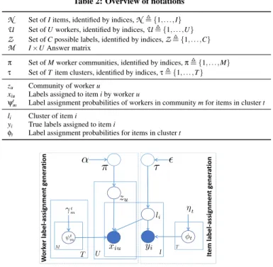
are modelled as observed variablesx∈(2Z)I×U, wherexiudenotes the set of labels assigned to itemiby workeru. Further,y∈(2Z)I _{are random variables modelling the true labels} of all items. True labels may be known for some items, which is captured by a set of observed variablesy⊆y. In general,ymay be empty. The values of variablesxandycan be represented as aC -dimensional vector, such that each of its components is set to one, if the respective label is present. Thus, we can consider the observed values ofxandyas samples from a Multinomial distribution.

Worker communities, item clusters, and label selection are mod-elled as follows (Fig. 2 shows a graphical representation):

Worker Communities. There is a finite set of worker communi-tiesπ, identified by indices,π,{1, . . . ,M}, that partition the set of

workers and are not known in advance. The (unknown) assignment of workers to communities is captured by a set of random vari-ablesz∈πU, such thatzudenotes the community of workeru. We generateπnonparametrically using a Chinese Restaurant Process (CRP). Following [20], it can be interpreted as the induced distribu-tion over the partidistribu-tion space by a Dirichlet Process [9]. Technically, ifπfollows a CRP distribution,π∼CRP(α), the samples from this prior follow the following distributions

p(zu=m|z−u,π,α)∝

(

n−mu if∃zu0∈_z−u:_zu0=_m

α otherwise

wherez−u=z\ {zu}andn−muis the number of elements inz−uwith communitym. As shown by Sethuraman [29],πcan be constructed using a stick-breaking process as follows. Letπ0m,m=1,2,3, . . .be sampled from a Beta distribution Beta(1,α). Then, the community proportionπmis calculated using the above sticksπ0m, such that

π1=π01, . . . ,πm=π0m m−1

∏

j=1 1−π0j ,· · · (1)

When conducting inference, we will only estimate the stick distri-butionπ0since the original distributionπcan be calculated directly

fromπ0as above. We further note that the nonparametric approach generalises the extreme cases. IfMtends to infinity, each worker is a single community (e.g., no two workers provide similar answers). IfMtends to zero, all workers form a single community (e.g., only expert workers) and the result is similar to majority voting.

Item Clusters.To model clusters of similar items, which tend to get assigned the same sets of labels, we follow the approach intro-duced for worker communities. There is a finite setτof clusters, identified by indices,τ,{1, . . . ,T}, that partition the set of items and are not known in advance. The (unknown) assignment of items to these clustered is captured by random variablesl∈τI, such that

lidenotes the cluster of itemi. Again,τis generated nonparametri-cally by a Chinese Restaurant Process, i.e.,τ∼CRP(ε).

The assignment of sets of labels to item clusters is modelled as a generation from a Multinomial distribution. For clustert, this distribution is parameterised byφt,{φt,1, . . . ,φt,C}, whereφt,cis the probability that a given item in clustertwill have the labelc. Items in a cluster may have different true labels as a result of the generating random process—yet, being in the same cluster, they are similar and thus share the labelling probabilities.

Label Selection. We model the labels obtained from workers as being generated from a Multinomial distribution over the labels of an item cluster, given a specific worker community. Each worker is characterised by aC×T confusion matrixψm, wheremis the community that the worker belongs to. We denote byψtma col-umn vector ofC-dimensions, which contains the probabilities that a worker in communitymassigns the respective labels given an item of clustert. This model has the advantage that, instead of con-sidering exponentially many subsets of labels, it is grounded in the number of all possible item clusters, which is tractable in practice.

For illustration, we consider a setting with four labels {1: girl, 2: boy, 3: dog, 4: cat}, two item clusters {1: people, 2: animal}, and two worker communities {1: trustworthy, 2: problematic}. Then, having a confusion matrix column vectorψ1₁= [0.5,0.5,0,0]means that workers of community 1 (trustworthy) assign an item of clus-ter 1 (people) the label 1 (girl), 2 (boy), 3 (dog), or 4 (cat) with probability 0.5, 0.5, 0, or 0, respectively.

Table 2: Overview of notations

N Set ofIitems, identified by indices,N,{1, . . . ,I}

U Set ofUworkers, identified by indices,U,{1, . . . ,U}

Z Set ofCpossible labels, identified by indices,Z,{1, . . . ,C}

M I×UAnswer matrix

π Set ofMworker communities, identified by indices,π,{1, . . . ,M} τ Set ofTitem clusters, identified by indices,τ,{1, . . . ,T}

zu Community of workeru

xiu Labels assigned to itemiby workeru

ψtm Label assignment probabilities of workers in communitymfor items in clustert

li Cluster of itemi

yi True labels assigned to itemi

φt Label assignment probabilities for items in clustert

Multi-label BNP Crowdsourcing

I W o rk e r la b e l-a ss ig n m e n t g e n e ra ti o n It e m l a b e l-a ss ig n m e n t g e n e ra ti o n

Figure 2: Graphical representation of the cBCMC model

Generative Process. Let Cat and Multi be Categorical and Multi-nomial distributions, respectively. Then, the generative process for the cBCMC model is defined as follows:

(1) For each item in

N

(right-hand side of Fig. 2): a) Generate the cluster for each item:li|τ∼Cat(τ)

b) Generate the labels for each item from the cluster:

yi|li,φ∼Mult φli

(2) For each worker in

U

(left-hand side of Fig. 2):

a) Generate the community for each worker:zu|π∼Cat(π)

b) Generate the set of assigned labels for each worker and item from the labels of the item cluster and the confusion matrix of the worker’s community:

xiu|zu,li,ψ∼Multψlziu

Model Parameters. The cBCMC model is nonparametric since the number of worker communities inπ and the number of item clusters inτare not known in advance—they change with more

observations (xandy) becoming available.

In a Bayesian setting, we use the following priors for the param-eters related to the worker communities and item clustering (Dir being a Dirichlet distribution):

π∼CRP(α) ψtm∼Dir γtm

τ∼CRP(ε) φt∼Dir(ηt)

with 1≤t≤T and 1≤m≤M. Bothτandπare unknown.

3.3

Inference

Inferring the parameters of the cBCMC model is, in fact, the estimation of values of the above priors (α,ε,γ,η). This is

equiv-alent to inferring the posterior distribution of the unobserved vari-ables (π,τ,z,l,ψ,φ) under the observed variables (x,y), which is

p(π,τ,z,l,ψ,φ|x,y), or p(π0,τ0,z,l,ψ,φ|x,y)using the

stick-breaking representation forπandτ(see Eq. 1).

Approaches for (approximate) inference for statistical models can be classified into simulation methods and deterministic vari-ational methods. The use of simulation such as Markov Chain Monte Carlo is problematic when applied to large-scale data sets

since convergence cannot be predicted. Thus, we resort to varia-tional inference. Specifically, we propose a novel scalable method that follows the principles of variational Bayesian inference (VB).

In variational inference, instead of computing the posterior dis-tribution directly, we infer an approximationq(π0,τ0,z,l,ψ,φ),

re-ferred to as variational distributions: q π0,τ0,z,l,ψ,φ= q π0|ρq τ0|υ U

∏

u=1 q(zu|κu) I

∏

i=1 q(li|ϕi) M

∏

m=1 T

∏

t=1 q ψtm|λtm T

∏

t=1 q(φt|ζt)

whereq(zu|κu)andq(li|ϕu)areM-dimensional andT -dimen-sional Multinomial distributions; andq(ψtm|λtm)andq(φt|ζt)are

C-dimensional Dirichlet distributions.

For the variational distributionsq(π0|ρ)andq(τ0|υ)we rely on a stick-breaking truncation representation for a Chinese Restaurant Process similar to those in [3], which are truncated toM andT, respectively. The variational distributions are:

q π0|ρ= M−1

∏

m=1 Beta π0m|ρm1,ρm2 q τ0|υ= T−1

∏

t=1 Beta τ0t|υt1,υt2

To approximate the posterior distributionspby variational distribu-tionsq, we use theKL-divergence between them,KL(q|p). With Θ,{π0,τ0,z,l,ψ,φ}, it is defined as: KL(q|p),− ˆ q(Θ)lnp(Θ|x,y) q(Θ) dΘ =− ˆ q(Θ)lnp(Θ,x,y) q(Θ) dΘ+lnp(x,y) ≥ − ˆ q(Θ)lnp(Θ,x,y) q(Θ) dΘ,−

L

(Θ)

L

(Θ) is calledevidence lower bound(ELBO) and denotes the variational objective function. Using variational theory [16], tak-ing derivatives of this lower bound with respect to each variational parameter, we derive the following coordinate ascent updates [3]. Local Updates. We first update local variables (connected to a single data point), i.e.,zandlin our model. We update the respec-tive distributionsq(zu|κu)andq(li|ϕi)as follows (details on the computation of these equations are given in Appendix A):

κum∝exp I

∑

i=1 T

∑

t=1 ϕitElnp xiu|ψtm +E[lnπm] ! (2) ϕit∝exp(E[lnp(yi|φt)] +E[lnτt]) (3)

Global Updates. Next, we consider the updates for global (or outer) variables (connected to multiple data points), i.e.,π,τ,ψ, and

φin our model. We updateq(π0|ρ)andq(τ0|υ)by means of:

ρm1=1+ U

∑

u=1 κum ρm2=α+ U

∑

u=1 M

∑

l=m+1 κul (4) υt1=1+ I

∑

i=1 ϕit υt2=ε+ I

∑

i=1 T

∑

l=t+1 ϕil (5)

Here,α,ε>0 are ‘prior beliefs’ on the actual number of worker

communities and item clusters. Yet, their effects are marginal, as the updates are dominated by the observed information (κandϕ).

Distributionsq(ψtm|λtm)andq(φt|ζt)are update by means of:

λtmc=λtm0+ I

∑

i=1 ϕit U

∑

u=1 κumxiu (6) ζtc=ζt0+ I

∑

i=1 ϕityi (7) We summarize our inference algorithm to learn the model param-eters in Algorithm 1. It iteratively updates local paramparam-eters (κ,ϕ) and global parameters (ρ,υ,λ,ζ). The observed data (x,y) is used

in the updates of these parameters whenever their associated vari-ables are connected to the observed varivari-ables. Note that many up-dates of variables are independent, which can be exploited to scale up the performance. For instance, the individual updates ofκ

pa-rameters andϕparameters can be parallelised.

Algorithm 1Variational Inference for the cBCMC Model Input :Worker answersxand known true labelsy

Output:Estimated model parametersλ,ζ,ρ,υ,κ,ϕ 1 Random initialisation ofλ,ζ,ρ,υ,κ,ϕ

2 whilenot convergeddo

// Update the local variables

3 foru←1, . . . ,U and m←1, . . . ,MdoUpdateκumusing Eq. 2 ;

4 fori←1, . . . ,I and t←1, . . . ,Tdo Updateϕitusing Eq. 3 ;

// Update the global variables 5 form←1, . . . ,Mdo

6 Updateρm1andρm2using Eq. 4

7 fort←1, . . . ,T and c←1, . . . ,CdoUpdateλtmcusing Eq. 6 ;

8 fort←1, . . . ,Tdo

9 Updateυt1andυt2using Eq. 5

10 forfor c←1, . . . ,CdoUpdateζtcusing Eq. 7 ;

11 returnλ,ζ,ρ,υ,κ,ϕ

3.4

Prediction

To solve the multi-label answer aggregation problem, we con-struct a deterministic assignmentd:

I

→2C using the maximum likelihood principle (MAP) [7]. After approximating the values of model parameters

P

,{α,ε,γ,η}, we predict the labels of

non-grounded items. Technically, given an itemi, we denote byxUi,

{xvi|v∈Ui}the labels assigned by the workersUiwho provided answers for this item. Further,

D

,{x,y}denotes the assigned la-bels as well as known lala-bels as used in the inference. We now com-puteyiusing MAP estimation of the probabilityp(yi|xUi,

D

,

P

):

y∗_i =argmax yi p(yi|xUi,

D

,

P

) =argmax yi p(yi,xUi|

D

,

P

) (8) sincep(yi|xUi,

D

,

P

) =p(yi,xUi|

D

,

P

)/p(xUi|

D

,

P

), there is

no direct dependency betweenyi andxUi in the graphical

repre-sentation, and the divisor does not depend onyi. The above for-mulation of the conditional probability ofyi, i.e. p(yi|xUi,

D

,

P

),

has the advantage that it covers diverse crowdsourcing settings. For instance, the absence of known true labels (y=0/in

D

={x,y})

or a separation of training data and testing data (xUi*x) can be

directly encoded in this formulation.

To compute p(yi,xUi|

D

,

P

), we factorise over all

probabilis-tic dependencies in the graphical model representation. Using the derivation outlined in Appendix C, we arrive at the following form:

p(yi,xUi|

D

,

P

) = T

∑

t=1 ϕit

_∏

u∈Ui M

∑

m=1 κump xui|ψ(mt)MAP ! p yi|φMAPt

whereψ(mt)MAPandφMAP_t are maximum a posteriori (MAP) esti-mates (aka modes) of the inferred distributions ofψtmandφt.

However, the maximization problem in Eq. 8 is a zero-one inte-ger problem, which is known to be NP-hard—the exhaustive search needs to explore 2C−1 combinations of labels. Against this back-ground, we may use a greedy search algorithm to approximate the modey∗_i of the above distribution. Initially, all elementsy∗_ic

of the vector y∗_i are set as zeros. Then, we proceed iteratively and, in each iteration, set to one the elementyic∗_{that leads to the} largest increase of p y∗_i,xUi|

D

,

P

. This procedure terminates oncep y∗_i,xUi|

D

,

P

can not be further increased. The final con-figuration ofy∗_i will be the instantiation value for the deterministic assignment. Note that this instantiation can be done independently for all items, so that this step can be parallelised.

4.

INCREMENTAL COMPUTATION

The inference and prediction methods introduced above for the cBCMC model solve the multi-label answer aggregation problem in a static setting. However, in many cases, tasks are not answered immediately when posted on a crowdsourcing platform. Rather, the set of worker answers is gradually building up over time and intermediate aggregation results are valuable from an application point of view [35]. For instance, intermediate results may indicate that a task is too difficult for workers, so that it shall be re-designed. Also, if intermediate results are of high quality, the crowdsourcing process can be terminated early to save cost.

We cater for such an online setting by means of incremental computation for the cBCMC model. We present an inference al-gorithm that incrementally updates the model parameters based on new data, which are then used for predicting the true labels of all items. In each learning iteration, we maintain only the most recent parameter values, thereby avoiding the cost of repeatedly building the model from the complete set of answers. While this approach comes with a modest reduction in aggregation quality (explored in our experiments), it greatly improves aggregation efficiency.

4.1

Incremental Learning with

Stochastic Variational Inference

The deterministic variational inference presented in the previous section for the static setting maximises the EBLO function

L

(Θ)

using coordinate-ascent for each of the parameters of variational distributions. To realise incremental learning, we rely on stochastic variational inference [13] and apply stochastic optimization to the EBLO function based on newly received data.

Technically, data is received as a series of batchesb=1,2, . . .. Each batchbcontains the answers of a fixed number of workers

U

b (withUb being the cardinality of

U

b) for a set of items

N

b. We consider new answers as a subsample and, based thereon, derive a stochastic gradient. Specifically, we compute the difference∇ be-tween old and new values of each parameter. Following [13, 33], we classify variational distributions as beingglobalorlocal. In our setting, q(li|ϕi), q(π0|ρ), q(τ0|υ), q(ψtm|λtm), andq(φt|ζt) are global, whereasq(zu|κu)is local (ϕnow becomes global as

we consider multiple items in one update).

Natural Gradients.For the local distribution, we reuse the update formulation given for VB inference (i.e., Eq. 2). The respective dis-tribution is connected to a single data point, which can be computed directly from the new data. In contrast, for the global distributions, natural gradients are obtained for each variable over allu∈

U

bas follows (the derivation can be found in Appendix B):

∇_λt m

L

u= −λtm+γtm+U∑i∈Nbϕitκumxiu U (9) ∇ζt

L

u= −ζt+η+∑i∈Nbϕityi U (10) ∇ρm1

L

u= −ρm1+1+Uκum U (11) ∇ρm2

L

u= −ρm2+α+U∑Ml=m+1κum U (12) ∇υt1

L

u= −υt1+1+∑i∈Nbϕit U (13) ∇υt2

L

u= −υt2+ε+∑Tl=t+1∑i∈Nbϕil U (14)

The natural gradient forq(li|ϕi)is difficult to compute since the mean-parameterisation requires the constraints ∑Tt=1ϕit=1 and 0≤ϕit≤1 to be satisfied. Hence, we prefer to work with a minimal canonical parameterisation in exponential family form, parametris-ing the distribution byµinstead ofϕ:

q(li|µi) =exp(hµi,S(li)i −B(µi))

whereµi= h

µi1, . . .µi(T−1) iT

is aT−1-dimensional vector param-eter,B(µi) =1+∑Tt=−11exp(µit)is a normalisation function, and

S(l) = [I(l−1), . . . ,I(l−T+1)]Tis a sufficient statistic function. The idea of sufficient statistics is to only maintain the minimal/suf-ficient information instead of all data points to compute the proba-bility distribution. In our case, the sufficient function is defined as aT−1-dimensional binary vector, containing a value of one only at positionl. That is,I(x)is an indicator function,I(x) =1 ifx=0; andI(x) =0, otherwise. The natural gradient for parameterµis:

∇µit

L

u=

−µit+E[εt]−E[εT] +U(ait−atT)

U (15)

whereait=∑Mm=1κumE[lnp(xiu|ψtm)]fort=1, . . . ,T. To derive

ϕfromµ, we use the following transformation:

ϕit= exp(µit) 1+∑T_t=−11exp(µit) fort=1, . . .T−1 (16) ϕiT= 1 1+∑Tt=−11exp(µit) (17) Learning Rate. In incremental learning, a learning rateωbneeds to be specified as a function of the batch indexb. To ensure the convergence of the gradients,ωbshall satisfy two conditions:

∞

∑

b=1 ωb=∞ and ∞

∑

b=1 ω2b<∞.

In general, a too small value ofωb might lead to non-optimality; a too large value might lead to non-convergence. The learning rate actually depends on r, aka the forgetting rate. Ifr is large,

ωb becomes small, and the old parameter values are only slightly changed. Finding an appropriate value forris specific to a dataset. As suggested in [13], we varyr∈(0.5,1]in our experiments. Online Updates.Using the above gradients, the updates of all nec-essary parameters in the online setting become:

λ←λ+ωb U Ubu∈U

∑

b ∇λLu ζ←ζ+ωb U Ubu∈U

∑

b ∇ζLu (18) ρ←ρ+ωb U Ubu∈

∑

Ub ∇ρLu υ←υ+ωb U Ubu

∑

∈Ub ∇υLu (19) µ←µ+ωb U Ub_u∈U

∑

b ∇µLu (20)

The algorithm for incremental learning for the cBCMC model is illustrated in Algorithm 2. In each iteration, a pre-defined number of answers are collected from the crowd. Based on the new data, we compute the natural gradients and update the model parameters.

Algorithm 2Stochastic Variational Inference for the cBCMC model Input :Continuously updated worker answersxand known true labelsy

Output:Estimated model parametersλ,ζ,ρ,υ,κ,ϕ 1 Random initialisation ofλ,ζ,ρ,υ,κ,ϕ

2 b←1// The batch index 3 whilemore answers are availabledo

4 Fetch theb-th batch of answers of usersUbfor itemsNband setb←b+1

// Update the local variables

5 foru∈Uband m←1, . . . ,MdoUpdateκumusing Eq. 2. ;

// Update the global variables 6 Compute the natural gradients using Eq. 9 to 15. 7 Set learning rateωb= (1+b)−r

8 Updateλ,ζ,ρ,υ,µusing Eq. 18 to 20. 9 Computeϕusing Eq. 16 to 17. 10 returnλ,ζ,ρ,υ,κ,ϕ

4.2

Online Prediction

Online prediction enables us to perform the instantiation of la-bels incrementally, upon the arrival of new answers. Different from the inference procedure for incremental learning, online prediction does not compute the difference between the old and new labels as-signments. The reason is that the most recent parameter values con-stitute the probability distributions of all data obtained so far. Each time new answers are obtained, the parameter values are updated and their values can be used to generate the corresponding approxi-mated posterior distributions of model variables required for instan-tiation, i.e.,q(b)(li|ϕi),q(b)(zu|κu),q(b)(ψtm|λtm),q(b)(φt|ζt),

q(b)(π0|ρ)andq(b)(τ0|υ), whereb=1,2, . . .is the batch index. These posteriors are approximations of their offline counterparts and, thus, are used as input of the instantiation procedure in §3.4.

5.

EVALUATION

We evaluated our approach to multi-label answer aggregation along several dimensions. We first elaborate on our experimental setup (§5.1), before evaluating the following aspects:

• The effectiveness of the cBCMC model for answer aggregation in a static setting (§5.2).

• The effectiveness of the cBCMC model when using incremen-tal computation in an online setting (§5.3).

• The efficiency of incremental computation (§5.4).

• The importance of representing worker communities and item clusters in the cBCMC model (§5.5).

5.1

Experimental Setup

Task Design.Aiming at a realistic evaluation setup, we follow best practices on task design for crowdsourcing:

Batch processing: Each task consists of multiple items that are to be labelled by a single user. To mediate the trade-off between the overhead of switching tasks and the cognitive load of a single task, we follow recent studies on crowdsourcing effectiveness [14], suggesting a task size of 10 items.

Pricing:We vary the price for a task over the datasets based on the difficulty of the respective tasks. Considering that a simple task would take five minutes to complete and that the average wage of workers is around 2.00$/h [27], we set the task price to 0.1$, 0.2$, and 0.3$ for simple, medium, and difficult tasks, respectively. Datasets. Our experiments have been conducted using five real-world datasets, spanning diverse application scenarios:

(1) Image annotation:From the NUS-WIDE set of tagged web images [6], we randomly selected 2000 images, such that tags are uniformly distributed. Each image has up to 10 tags, which serve as ground truth in our experiments. Workers were asked to assign a subset of 81 possible tags to each image.

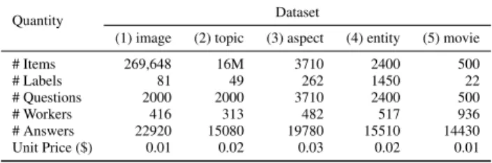
Table 3: Statistics for real-world datasets

Quantity Dataset

(1) image (2) topic (3) aspect (4) entity (5) movie

# Items 269,648 16M 3710 2400 500 # Labels 81 49 262 1450 22 # Questions 2000 2000 3710 2400 500 # Workers 416 313 482 517 936 # Answers 22920 15080 19780 15510 14430 Unit Price ($) 0.01 0.02 0.03 0.02 0.01

(2) Topic annotation: We relied on a random sample of 2000 Twitter messages from the collection that was used in the TREC 2011 Microblog track [22]. This dataset assigns up to five topics (from a set of 49 topics) to each tweet and, again, we ensured a uniform distribution of topic labels in our sample.

(3) Aspect extraction:This dataset is about assigning evaluation aspects (e.g.,priceormenu) to restaurant reviews [11]. The ground truth, provided by [23], assigns up to five aspects (out of 262) to 3710 reviews. We designed crowdsourcing tasks that asked work-ers to assign a subset of 20 possible labels to each review. The set of possible labels contains the true labels and is filled up with the labels that have the highest co-occurrences with the true labels.

(4) Entity extraction: The T-NER dataset [26] contains 2400 tweets, to which entities (of ten categories such as products or fa-cilities) shall be assigned. It also includes the ground truth for all tweets. We asked workers to tag each word of a tweet as being an entity or non-entity, so that each tweet is assigned a set of entities.

(5) Movie tagging: This dataset has been created by crawling the IMDB website, randomly selecting 500 movies from a total of 22 genres. As such, the ground truth directly stems from the IMDB website. Workers have been asked to assign genres to these movies. We employed workers to perform item labelling using the Crowd-Flower platform [31]. In total, we spent a total budget of 8772 tasks for all datasets and ended up having a repository of 87720 label an-notations for 10610 items from 2664 users, see also Table 3.

The resulting datasets cover diverse crowdsourcing scenarios: the distribution of worker answers is skewed in datasets (1) and (5), whereas it is normal in (3); tasks in datasets (2), (3), and (4) require understanding of unstructured text, which is more difficult than the tasks in (1) and (5); labels in (1), (2), and (4) are strongly correlated, whereas there is little correlation between labels in (5). Metrics.In multi-label answer aggregation, results can be partially correct. We therefore rely on the set-based definition of precision and recall to evaluate the individual correctness of each item. Per itemi,individual precision Piis the ratio of correctly predicted la-bels and the total number of predicted lala-bels, whereasindividual re-call Riis the ratio of correctly predicted labels and the total number of true labels. For a complete dataset,precision Pandrecall Rare the respective averages over all items. WithYi,Sj∈Z{j|yi j=1} andY_i∗,S

j∈Z{j|y∗i j=1}, the measures are defined as:

Pi, |Yi∩Yi∗| |Y_i∗| Ri, |Yi∩Yi∗| |Yi| P, I

∑

i=1 Pi I R, I

∑

i=1 =Ri I

Baseline. We compare our approach against a baseline using ma-jority voting, which is the only available aggregation method for the multi-label setting [4]. To ensure a fair comparison, we adapt the standard approach (see §2) by injecting knowledge on the re-sult cardinality. That is, the baseline ranks labels per item by their number of appearances in the answers. We then consider the top-k

labels, withkbeing the number of labels assigned by our approach (ties are resolved randomly and we average of multiple solutions). Experimental Environment. All experimental results have been obtained on an Intel Core i7 system (3.4GHz, 12GB RAM), using parallelisation (as mentioned in §3 and §4) whenever possible.

ima

getopicaspec

t

ent

ity

mo

vie

0.0

0.2

0.4

0.6

0.8

1.0

∆

Pr

ec

isi

on

baseline cBCMC

ima

getopicaspec

t

ent

ity

mo

vie

0.0

0.2

0.4

0.6

0.8

1.0

∆

Re

ca

ll

baseline cBCMC

(a)Sparsity level = 25%

ima

getopicaspec

t

ent

ity

mo

vie

0.0

0.2

0.4

0.6

0.8

1.0

∆

Pr

ec

isi

on

baseline cBCMC

ima

getopicaspec

t

ent

ity

mo

vie

0.0

0.2

0.4

0.6

0.8

1.0

∆

Re

ca

ll

baseline cBCMC (b)Sparsity level = 50% Figure 3: Effects of sparsity(compared to performance at sparsity level = 0% as ratio)

imagetopicaspec

t

ent

ity

mo

vie

0.0

0.2

0.4

0.6

0.8

1.0

∆

Pr

ec

isi

on

baseline cBCMC

imagetopicaspec

t

ent

ity

mo

vie

0.0

0.2

0.4

0.6

0.8

1.0

∆

Re

ca

ll

baseline cBCMC

(a)Spammer ratio = 10%

imagetopicaspec

t

ent

ity

mo

vie

0.0

0.2

0.4

0.6

0.8

1.0

∆

Pr

ec

isi

on

baseline cBCMC

imagetopicaspec

t

ent

ity

mo

vie

0.0

0.2

0.4

0.6

0.8

1.0

∆

Re

ca

ll

baseline cBCMC (b)Spammer ratio = 20% Figure 4: Effects of spammers(compared to performance at spammer ratio = 0% as ratio)

5.2

Effectiveness in a Static Setting

Accuracy.We first evaluate the accuracy of our approach based on the cBCMC model against the baseline method in a static setting. That is, we measure individual precision and individual recall of each item of the aforementioned five datasets.

image topic aspectentitymovie 0 20 40 60 80 100 Fre qu en cy (% ) 0.25 0.5 0.75 1.0 cBCMC baseline

Figure 5: Individual Precision

image topic aspectentitymovie 0 20 40 60 80 100 Fre qu en cy (% ) 0.25 0.5 0.75 1.0 cBCMC baseline

Figure 6: Individual Recall Fig. 5 and 6 show the obtained results in terms of histograms over all items, where the bins are[0,0.25],(0,25,0.5],(0.5,0.75], and

(0.75,1]. We observe that our approach outperforms the baseline methods for all datasets: there are notably more items with high individual precision and recall (bins(0.5,0.75]and(0.75,1]) in all cases. We further observe that the absolute number of items for which we obtain accurate results varies across the datasets:aspect

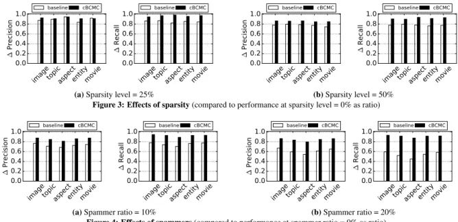
tasks are difficult, which leads to the lowest precision and recall values. For datasetimage, we observe better results than formovie, since we can exploit co-occurrence dependencies between labels. Robustness against Sparsity.In crowdsourcing scenarios, the an-swer matrix is typically sparse: most workers process only a few of the items of a particular application. We investigate the effect of sparsity on aggregation accuracy by randomly removing a certain share of the answers, leaving 25% or 50% of the data per dataset. We then measure precision and recall, averaged over 100 runs.

As illustrated in Fig. 3, in general, precision and recall decrease if answers are removed. However, answer aggregation based on our cBCMC model is affected less by data sparsity compared to the baseline method. For instance, forimagetasks, when removing half of the input data (sparsity level 50%), the precision of our method is already 86% of the precision obtained using all answers. The baseline, in turn, achieves only 78% of the precision obtained using all answers in this case. This effect is due to the notion of worker communities in the cBCMC model that help to identify consistent answers for an item even if it was processed only by a few workers.

Robustness to Spammers.As discussed in §2, crowdsourcing ap-plications suffer from faulty workers, such as random and uniform spammers, which can account for up to 40% of the worker popula-tion [8, 32]. Even though we may be able to detect different types of workers (based on their characteristics), the predicted labels may be incorrect, since faulty answers can be dominating. We investi-gate this aspect by adding answers of spammers to the datasets, such that they account for 10% or 20% of the data.

As expected, the results in Fig. 4 show that precision and recall decrease when spammers are included. However, our approach is much less affected by spammers as is the baseline method, in par-ticular for large amounts of spammers (20%). For example, for theaspectdataset, the precision of the baseline method decreases from 0.49 to 0.43, whereas it stays nearly constant with our ap-proach, achieving 0.71 and 0.70, respectively. This highlights that our approach can not only detect communities of spammers, but also limits their influence on the aggregation result.

5.3

Effectiveness in an Online Setting

Incremental computation for the cBCMC model as introduced in §4 aims at increasing the efficiency of computation. Yet, it may come at the expense of decreased effectiveness, i.e., lower accuracy in terms of precision and recall. We therefore compare the accuracy of the baseline method with the cBCMC model, once with the in-ference mechanisms for a static setting (offline) and once with the approach with incremental learning (online). To this end, we simu-late an online setting by randomly selecting new worker answers to represent newly arriving data, in steps of 10% of the dataset size. For the non-incremental methods (baseline and offline), this setup corresponds to a step-wise increase of the sparsity level from 10% to 100% and the prediction is always based on the complete set of answers received so far.

10 20 30 40 50 60 70 80 90 100 Data Arrival (%) 0.3 0.4 0.5 0.6 0.7 0.8 0.9 Pre cisi on image dataset baseline online offline 10 20 30 40 50 60 70 80 90 100 Data Arrival (%) 0.3 0.4 0.5 0.6 0.7 0.8 Re ca ll image dataset baseline online offline

The result for theimagedataset is shown in Fig. 7. We notice that indeed, precision and recall are worse when using incremen-tal computation for the cBCMC model. Yet, even with incremenincremen-tal computation, the results are significantly better than those of the baseline. For example, when the share of available answers in-creases from 10% to 50%, the precision of the cBCMC model with incremental computation increases from 0.49 to 0.70, while for the baseline, this increase is only from 0.45 to 0.50. This underlines that the summarised information about item clusters and worker communities maintained by our incremental inference method still enables more accurate aggregation compared to the baseline.

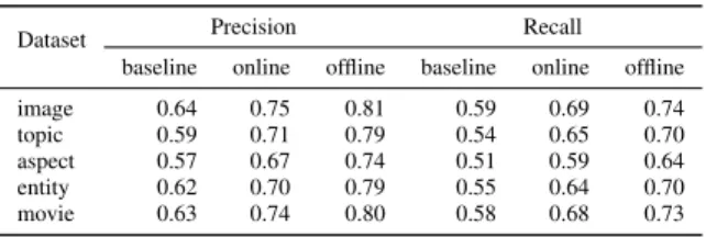
Table 4: Effects of data arrival (at 100%)

Dataset Precision Recall

baseline online offline baseline online offline image 0.64 0.75 0.81 0.59 0.69 0.74 topic 0.59 0.71 0.79 0.54 0.65 0.70 aspect 0.57 0.67 0.74 0.51 0.59 0.64 entity 0.62 0.70 0.79 0.55 0.64 0.70 movie 0.63 0.74 0.80 0.58 0.68 0.73 The result for theimagedataset in Fig. 7 is representative for all datasets. Table 4 shows precision and recall obtained with the three methods after all answers have been processed. While incremental computation based on the cBCMC model incurs a moderate drop in accuracy compared to the non-incremental approach, it achieves consistently higher accuracy than the baseline method.

5.4

Efficiency of Incremental Computation

We now turn to the efficiency of incremental computation for the cBCMC model and measure the runtime of the inference mech-anism for a static setting (offline) and the runtime of the incre-mental inference (online), in relation to the size of the input data. To have a controlled experimental setup, we generated a synthetic dataset, comprising 10,000 items and 500 workers. The actual input data has been generated randomly by the generative process of the cBCMC model, for which the priors are set based on the inference results for the five real-world datasets. We consider the average over these five configurations and over 100 experiment runs. In the experiment, we vary the density, taking between 5% and 30% of the complete answer matrix as input. Non-incremental inference is said to converge, if all model parameter differences in two consecu-tive inference iterations are below 10−3. For incremental inference, we set the batch size to 50 answers and the forget rate to 0.8.

5 10 15 20 25 30 Data Density (%) 0 2 4 6 8 10 Tim e( × 10 3 s) online offline

Figure 8: Runtime of inference mechanisms for the cBCMC model

As shown in Fig. 8, the incremental inference mechanism is in-deed much more efficient than the non-incremental one. Inference in a static setting is non-linear: the computation requires iteration over two dimensions of the input data and an increased model com-plexity means that more iterations are needed to converge. Incre-mental inference, in turn, is performed on a fixed number of newly received answers and, therefore, scales linearly.

5.5

Importance of Model Aspects

Finally, we assess the importance of explicitly capturing worker communities and item clusters by comparing the accuracy of our cBCMC model with two simplified versions: No_Z removes the

community structure (variablez) from the model, i.e., each worker is a singleton community;No_Lremoves the item cluster structure (variablel), i.e., each item represents a singleton cluster. However, theNo_Lmodel turned out to be intractable for all except themovie

dataset, since all possible subsets of labels have to be considered.

imagetopicaspecentt itymovie 0.0 0.2 0.4 0.6 0.8 1.0 Pre cisi on _cBCMC No_Z No_L

imagetopicaspecentt itymovie 0.0 0.2 0.4 0.6 0.8 1.0 Re ca ll cBCMC_{No_Z} No_L

Figure 9: Effects of model aspects

Fig. 9 shows that the cBCMC model consistently achieves the highest precision and recall. Improvements over theNo_Zmodel are particularly large for the more difficult datasets (topicand as-pect), since differentiation of workers is effective in these cases.

We further note that theNo_Zmodel achieves higher precision, but lower recall than theNo_Lmodel. This highlights that worker communities help to improve correctness by identifying faulty work-ers, whereas item clusters improve completeness by exploiting la-bel co-occurrence dependencies.

6.

RELATED WORK

Having discussed the context of answer aggregation in crowd-sourcing in §1 and §2, below, we focus on further related areas. Multi-label Problems. Multi-label problems have been solved in related research fields, such as multi-label classification [38], ordi-nal classification [18], and data streams classification [10]. Multi-label classification aims at learning classifiers to associate each item with a set of labels. Yet, different from the crowdsourcing setting, it is based on the features of the data itself, such as im-age pixels or textual indicators [38]. Ordinal classification studies a similar setting, yet assuming a natural ordering among labels. It can be traced back to multi-label classification through membership functions [18]. Our work considers a more generic relation between labels in terms of their co-occurrence for the items in a cluster. Data streams classification aims at multi-label classification in an online setting, processing data in a real-time manner [10].Despite the dif-ferences in the underlying classification problem (answer aggrega-tion is not based on features of the items that shall be labelled), this setting is similar to the online setting in crowdsourcing.

Multi-label problems have been studied in the context of crowd-sourcing before, yet the focus has been primarily on minimizing cost when posting tasks, see [5]. Another example is work on opti-mising the cost of hiring workers when generating training data for classifiers [4]. However, these approaches assume labels to be in-dependent and consider all workers equally—adopting some form of majority voting to aggregate answers. Answer aggregation for multi-label crowdsourcing that takes into account the worker com-munities, partial answer validity, label dependencies, and adaptivity of the aggregation model, in turn, has not been addressed before. Bayesian Models. Graphical probabilistic models have been suc-cessfully applied in various domains, such as image processing, video encoding, and machine learning [21]. Their main benefit is the ability to explicitly capture dependencies between random vari-ables, which often done by means of factor graphs. However, most attempts to use graphical models for multi-label answer aggrega-tion, e.g., [4], show two two major limitations: (1) the models are parametric, which enforces assumptions on the true distribution of crowdsourcing data, even though there is no ground truth available;

(2) they ignore worker communities, even though spammers may have a huge impact on the aggregation result, see [39].

To cope with the first limitation, Bayesian nonparametric mod-els may be used. Their flexibility in terms of a variable number of model parameters makes them well suited to characterise the distri-butions underlying real-world data. As discussed in §2.3, a first ap-plication of Bayesian nonparametric models to answer aggregation for single-label crowdsourcing was recently proposed by Moreno et al. [20]. In this work, we generalised these ideas and presented the cBCMC model for multi-label problems in crowdsourcing. Un-like the existing work, our model supports partial answer validity and exploits co-occurrence dependencies between labels.

7.

CONCLUSION AND FUTURE WORK

In this paper, we presented a novel Bayesian nonparametric ap-proach to aggregate multi-label crowdsourcing answers. The key features of the proposed cBCMC model are its ability to capture worker characteristics (by worker communities) and dependencies between the labels assigned to items (by item clusters). The for-mer ultimately improves precision by separating answers of faulty workers from those of reliable workers; the latter ultimately im-proves recall by exploiting co-occurrence dependencies to com-plete results. We further presented inference and prediction mech-anisms for the cBCMC model for both, static as well as online sce-narios. Our experimental results showed that answer aggregation based on the cBCMC model outperforms a baseline method by up to 134% in precision and recall, while being robust against spam-mers and the answer sparsity as often observed in crowdsourcing. In future work, we intend to lift our model to other types of crowd-sourcing tasks, such as ranking or assignment of continuous labels.

References

[1] Q. Abbas et al. “Pattern classification of dermoscopy im-ages: A perceptually uniform model”. In:JPR(2013), pp. 86– 97.

[2] Y. Amsterdamer et al. “Crowd Mining”. In:SIGMOD. 2013, pp. 241–252.

[3] D. Blei et al. “Variational inference for Dirichlet process mixtures”. In:Bayesian Anal.(2006), pp. 121–143. [4] J. Bragg et al. “Crowdsourcing multi-label classification for

taxonomy creation”. In:HCOMP. 2013.

[5] C. C. Cao et al. “Whom to ask?: jury selection for deci-sion making tasks on micro-blog services”. In:VLDB. 2012, pp. 1495–1506.

[6] T.-S. Chua et al. “NUS-WIDE: a real-world web image database from National University of Singapore”. In:CIVR. 2009, p. 48.

[7] A. P. Dempster et al. “Maximum likelihood from incomplete data via the EM algorithm”. In:J. R. Stat. Soc(1977), pp. 1– 38.

[8] D. E. Difallah et al. “Mechanical Cheat: Spamming Schemes and Adversarial Techniques on Crowdsourcing Platforms.” In:CrowdSearch. 2012, pp. 26–30.

[9] T. Ferguson. “A Bayesian analysis of some nonparametric problems”. In:AOS(1973), pp. 209–230.

[10] M. M. Gaber et al. “A survey of classification methods in data streams”. In:Data Streams. 2007, pp. 39–59.

[11] G. Ganu et al. “Beyond the Stars: Improving Rating Predic-tions using Review Text Content.” In:WebDB. Vol. 9. 2009, pp. 1–6.

[12] C. Gokhale et al. “Corleone: Hands-off Crowdsourcing for Entity Matching”. In:SIGMOD. 2014, pp. 601–612.

[13] M. D. Hoffman et al. “Stochastic variational inference”. In:

JMLR(2013), pp. 1303–1347.

[14] J. J. Horton et al. “The labor economics of paid crowdsourc-ing”. In:EC. 2010, pp. 209–218.

[15] N. Q. V. Hung et al. “An Evaluation of Aggregation Tech-niques in Crowdsourcing”. In:WISE. 2013, pp. 1–15. [16] M. Jordan et al. “An introduction to variational methods for

graphical models”. In:ML(1999), pp. 183–233.

[17] G. Kazai et al. “Worker types and personality traits in crowd-sourcing relevance labels”. In:CIKM. 2011, pp. 1941–1944. [18] W. Kotlowski et al. “On nonparametric ordinal classification with monotonicity constraints”. In:TKDE(2013), pp. 2576– 2589.

[19] K. Lee et al. “The social honeypot project: protecting online communities from spammers”. In:WWW. 2010, pp. 1139– 1140.

[20] P. G. Moreno et al. “Bayesian Nonparametric Crowdsourc-ing”. In:JMLR(2015), pp. 1607–1627.

[21] K. P. Murphy.Machine learning: a probabilistic perspective. MIT press, 2012.

[22] I. Ounis et al. “Overview of the trec-2011 microblog track”. In:TREC. 2011.

[23] J. Pavlopoulos et al. “Aspect term extraction for sentiment analysis: New datasets, new evaluation measures and an im-proved unsupervised method”. In:ACL. 2014, pp. 44–52. [24] A. J. Quinn et al. “Human computation: a survey and

taxon-omy of a growing field”. In:CHI. 2011, pp. 1403–1412. [25] V. C. Raykar et al. “Ranking annotators for crowdsourced

labeling tasks”. In:NIPS. 2011, pp. 1809–1817.

[26] A. Ritter et al. “Named entity recognition in tweets: an ex-perimental study”. In:ACL. 2011, pp. 1524–1534.

[27] J. Ross et al. “Who are the crowdworkers?: shifting demo-graphics in mechanical turk”. In:CHI. 2010, pp. 2863–2872. [28] S. Sen et al. “Tagging, communities, vocabulary, evolution”.

In:CSCW. 2006, pp. 181–190.

[29] J. Sethuraman. “A constructive definition of Dirichlet pri-ors”. In:Statistica Sinica(1994), pp. 639–650.

[30] C. Sun et al. “Chimera: Large-Scale Classification using Ma-chine Learning, Rules, and Crowdsourcing”. In:VLDB. 2014, pp. 1529–1540.

[31] http://www.crowdflower.com/.

[32] J. Vuurens et al. “How much spam can you take? an analy-sis of crowdsourcing results to increase accuracy”. In:CIR. 2011, pp. 48–55.

[33] C. Wang et al. “Online variational inference for the hierar-chical Dirichlet process”. In:AISTATS. 2011.

[34] F. L. Wauthier et al. “Bayesian bias mitigation for crowd-sourcing”. In:NIPS. 2011, pp. 1800–1808.

[35] T. Yan et al. “CrowdSearch: Exploiting Crowds for Accurate Real-time Image Search on Mobile Phones”. In:MobiSys. 2010, pp. 77–90.

[36] J. Yi et al. “Semi-crowdsourced clustering: Generalizing crowd labeling by robust distance metric learning”. In:NIPS. 2012, pp. 1772–1780.

[37] C. J. Zhang et al. “Reducing Uncertainty of Schema Match-ing via CrowdsourcMatch-ing”. In:VLDB. 2013, pp. 757–768. [38] M.-L. Zhang et al. “Multi-label learning by exploiting label

dependency”. In:KDD. ACM. 2010, pp. 999–1008. [39] B. Zhao et al. “A bayesian approach to discovering truth

from conflicting sources for data integration”. In: VLDB. 2012, pp. 550–561.

APPENDIX

A.

OFFLINE LEARNING WITH DETERMINISTIC VARIATIONAL INFERENCE

We provide the detailed computation of two equations:

κum∝exp I

∑

i=1 T

∑

t=1 ϕitElnp xiu|ψtm +E[lnπm] ! ϕit∝exp(E[lnp(yi|φt)] +E[lnτt]) by: E[lnp(xiu|ψ)] = C

∑

c=1 xiuc ψ λtmc −ψ

∑

c λtmc +lnΓ

∑

c xiuc+1 −

_∑

c lnΓ(xiuc+1) E[lnp(yi|φt)] = C

∑

c=1 xiuc ψ(ζtc)−ψ

∑

c ζtc +lnΓ

∑

c yic+1 −

_∑

c lnΓ(yic+1) E[lnπm] =Elnπ0m + m−1

∑

k=1 Eln 1−π0_k Elnπ0m =ψ(ρm1)−ψ(ρm1+ρm2) Eln 1−π0m =ψ(ρm2)−ψ(ρm1+ρm2) E[lnτt] =Elnτ0t + t−1

∑

k=1 Eln 1−τ0_k Elnτ0t =ψ(υt1)−ψ(υt1+υt) Eln 1−τ0_t=ψ(υm2)−ψ(υm1+υm2)

Here,ψ(·)is digamma function;Γ(·)is gamma function.

B.

ONLINE LEARNING WITH STOCHASTIC VARIATIONAL INFERENCE

In this online setting, we suppose that we have the number of workers and the number of answers from workers will be increased by time. The ELBO function that we need to optimize become:

L

=Elnp π0,τ0,z,l,ψ,φ,x,y

Elnp π0,τ0,z,l,ψ,φ,x,y=Elnp x|π0,τ0,z,l,ψ,φ+Elnp y|τ0,l,ψ,φ =

_∑

u,i Elnp xui|ψzuli +

_∑

u Elnp zu|π0 +

_∑

i Elnp yi|φli +

_∑

i Elnp li|τ0 +

_∑

m,t Elnp ψtm +

_∑

t E[lnp(φt)] + M−1

∑

m=1 E h lnpπ 0 m i + T−1

∑

t=1 E h lnpτ 0 t i =

_∑

u

∑

i Elnp xui|ψzuli +Elnp zu|π0 ! +

_∑

i Elnp yi|φli +

_∑

i Elnp li|τ0 +

_∑

m,t Elnp ψtm +

_∑

t E[lnp(φt)] + M−1

∑

m=1 E h lnpπ 0 m i + T−1

∑

t=1 E h lnpτ 0 t i Elnq π0,τ0,z,l,ψ,φ=

_∑

u E[lnq(zu)] +

_∑

i E[lnq(li)] +

_∑

m,t Elnq ψtm +

_∑

t E[lnq(φt)] + M−1

∑

m=1 E h lnq π 0 m i + T−1

∑

t=1 E h lnq τ 0 t i

Therefore, the global parameters now includeq(ψtm|λtm),q(φt|ζt),q(li|ϕi),q(π0|ρ)andq(τ0|υ). Their natural gradients are:

∂

L

u ∂λt_m = ∂ ∂λt_m

∑

_i E lnp xui|ψzuli + 1 UE lnp ψtm − 1 UE lnq ψtm ! ∂

L

ung ∂λtm =−λ t m+γtm+U∑iϕitκumT xj,1 U ∂

L

u ∂ζt = ∂ ∂ζt 1 U

∑

_i E lnp yi|φli + 1 UE[lnp(φt)]− 1 UE lnq ψtm ! ∂

L

ung ∂ζt = −ζt+η+∑iϕit[T(yi),1] U ∂

L

u ∂ρm1 = ∂ ∂ρm1 Elnp zu|π0+ 1 UE h lnp π 0 m i − 1 UE h lnq π 0 m i ∂

L

ung ∂ρm1 = −ρm1+1+Uκum U ∂

L

u ∂ρm2 = ∂ ∂ρm2 Elnp zu|π0+ 1 UE h lnp π 0 m i − 1 UE h lnq π 0 m i ∂

L

ung ∂ρm2 = −ρm2+1+U∑ M l=m+1κum U ∂

L

u ∂υt1 = ∂ ∂υt1 1 U

∑

_i E lnp li|τ0+ 1 UE h lnpτ 0 t i − 1 UE h lnqτ 0 t i ! ∂

L

ung ∂υt1 =−υt1+1+∑iϕit U

∂

L

u ∂υt2 = ∂ ∂υt2 1 U

∑

_i E lnp li|τ0+ 1 UE h lnpτ 0 t i − 1 UE h lnqτ 0 t i ! ∂

L

ung ∂υt2 =−υt2+1+∑ T l=t+1∑iϕil U

The natural gradient for the canonical parameterµof mean parameterϕis: ∂

L

u ∂µi = ∂ ∂µi E lnp xui|ψzuli + 1 U

∑

_i E lnp yi|φli − 1 U

∑

_i E[lnq(li)] ! = ∂ ∂µi E lnp xui|ψzuli + 1 U

∑

_i E lnp yi|φli − 1 U

∑

_i E[lnq(li)] ! ∂ ∂µiE lnp xiu|ψzuli = ∂ ∂µi

∑

t

∑

m κumElnp xiu|ψtm ϕit = h ai1−a1T, . . . ,ai(T−1)−a(T−1)T i_∂2_B(µi) ∂µi∂µ>_i Therefore: ∂

L

ung ∂µit =−µit+E[εt]−E[εT] +U(ait−atT) U whereait=∑mκumE[lnp(xiu|ψtm)] t=1, . . . ,T−1.

C.

PREDICTION

We have: p(yi,xUi|

D

,

P

) = ˆ p(yi,xUi|Θ)p(Θ|

D

,

P

)dΘ ≈ ˆ

p(yi,xUi|Θ)q(Θ)dΘ (from Variational Bayesian in the inference step)

Therefore, the true input of our prediction step is the approximated posterior variational distributions,q(ψtm|λtm),q(φt|ζt),q(π0|ρ)and

q(τ0|υ). We can use MAP estimation to obtain values forψtmand φt which are denotedψ(mt)MAP and φtMAPfrom this (approximated) posterior. The cluster proportion distributions, ,q(π0|ρ)andq(τ0|υ), are used as the full distributions.

ˆ p(yi,xUi|Θ)q(Θ)dΘ =

∑

li ˆ

∏

u∈Ui

∑

zu p(xui|zu,li,Θ)p(zu|Θ) p(yi|li,Θ)p(li|Θ)q(Θ)dΘ =

_∑

li p(li|υ) ˆ p(yi|li,φ)q(φ)dφ

∏

u∈Ui

∑

zu p(zu|κu) ˆ p(xui|zu,li,ψ)q(ψ)dψ =E h E[p(yi|li,φ)]q(φ) i q(li)

∏

u∈Ui E h E[p(xui|zu,li,ψ)]_q(ψ) i q(zu) E h E[p(yi|li,φ)]_q(φ) i q(li) = T

∑

t=1 ϕitE[p(yi|φt)] = T

∑

t=1 ϕitp yi|φMAPt E h E[p(xui|zu,li,ψ)]_q(ψ) i q(zu)q(li) = T

∑

t=1 ϕit M

∑

m=1 κumEp xui|ψtm = T

∑

t=1 ϕit M

∑

m=1 κump xui|ψ(mt)MAP

whereφMAPt andψ (t)MAP

m are MAP estimates (a.k.a. mode) of their variational distributionsq(φt|ζt) =Dir(ζt),q(ψtm|λtm) =Dir(λtm), which are well-known for Dirichlet distributions.