Technological Progress and the
Geographic Expansion of the Banking
Industry
Allen N. Berger and Robert DeYoung
Technological Progress and the Geographic Expansion of the Banking Industry
Allen N. Berger
Board of Governors of the Federal Reserve System Washington, DC 20551 U.S.A.
and
Wharton Financial Institutions Center Philadelphia, PA 19104 U.S.A.
Robert DeYoung
Federal Reserve Bank of Chicago Chicago, IL 60604 U.S.A.
June 2002
Key Words: banks, efficiency, mergers, productivity, technological progress. JEL Codes: G21, G28, G34, L11.
The opinions expressed do not necessarily reflect those of the Federal Reserve Board, the Chicago Reserve Bank, or their staffs. The authors thank Bruno Biais, Bill Brainard, Neil Esho, Dan Gropper, Chris James, Loretta Mester, Steven Ongena, Marco Pagano, Fabio Panetta, Tony Saunders, Rick Sullivan, John Wolken, Oved Yosha, and other participants at the JFI Symposium on Corporate Finance with Blurring Boundaries Between Banks and Financial Markets and the Yale University Conference on “The Future of American Banking: Historical, Theoretical, and Empirical Perspectives” and the Federal Reserve Bank of Chicago’s Bank Structure and Competition Conference for helpful comments, and Nate Miller and Dan Long for outstanding research assistance. Please address correspondence to Allen N. Berger, Mail Stop 153, Federal Reserve Board, 20th and C Streets. NW, Washington, DC 20551, call 202-452-2903, fax 202-452-5295, or email [email protected], or to Robert DeYoung, Federal Reserve Bank of Chicago, 230 South LaSalle Street, Chicago, IL 60604, 312-322-5396 (voice), 312-322-2357 (fax), [email protected].
Technological Progress and the Geographic Expansion of the Banking Industry Abstract
We test some predictions about the effects of technological progress on geographic expansion using data on banks in U.S. multibank holding companies over 1985-1998. Specifically, we test whether over time (a) parental control over affiliate banks has increased, and (b) the agency costs associated with distance from the parent have decreased. The data suggest that banking organizations exercise significant control over affiliates that has been increasing over time, and that the agency costs associated with distance have decreased somewhat over time. The findings are consistent with the hypothesis that technological progress has facilitated the geographic expansion of the banking industry.
Technological Progress and the Geographic Expansion of the Banking Industry 1. Introduction
Over the past few decades, the banking industry has been in a constant process of geographic expansion, both within nations and across nations. At one time, nearly all customers were served by locally-based institutions. In contrast, it is now much more likely that the bank or branch providing services is owned by an organization headquartered at a substantial distance away, perhaps in another state, region, or nation. To illustrate, the average distance between the largest bank and the other affiliate banks in U.S. multibank holding companies (MBHCs) increased from 123.35 miles to 188.91 miles between 1985 and 1998, as many MBHCs acquired banks in other states and regions.
It is well understood that bank deregulation has played a large role in the geographic expansion of this industry. In the U.S., a series of deregulations in the 1980s and early 1990s removed restrictions on intrastate and interstate banking, culminating with the Riegle-Neal Interstate Banking and Branching Efficiency Act of 1994, which permitted interstate branching in almost all states as of June 1997. In the European Union, the set of actions known as the Single Market Programme – especially the single license provision of the Second Banking Co-ordination Directive of 1989 – essentially allows banking organizations to expand continent-wide. In Latin America and other regions, explicit and implicit regulatory barriers to foreign bank entry have fallen, allowing banking organizations headquartered in other nations to gain significant local market shares.
What is less well understood is the role of technological progress in facilitating geographic expansion. In any industry, there are potential diseconomies to geographic expansion in the form of agency costs associated with monitoring junior managers in a distant locale. Improvements in information processing and telecommunications, such as computer networking and the Internet, may lessen these agency costs by improving the ability of senior managers located at the organization’s headquarters to control staff at distant subsidiaries. In the banking industry, there have also been advances in financial technologies that may allow banks to deal more efficiently with distant customers. Greater use of quantitative methods in applied finance, such as credit scoring, may allow banks to extend credit without geographic proximity to the borrower by “hardening” their credit information (Stein 2002). Similarly, the new products of financial engineering, such as derivative contracts, may allow banks to unbundle, repackage, or hedge risks at low cost without respect to the distance from the counterparty. These financial innovations may allow senior managers at MBHC headquarters to monitor decisions made by loan officers and managers at distant affiliate banks more easily, and evaluate and manage the
contributions of individual affiliate banks to the organization’s overall returns and risk more efficiently.
Some recent research discussed below suggests that technological progress may have led to significant revenue-based productivity improvements at banks in the 1990s. Given that U.S. banking organizations have had tremendous geographical expansion during this time period, the coincident productivity improvement is consistent with the hypothesis that these organizations have improved their control over distant affiliates and/or have reduced the agency costs associated with distance. Other recent research found that the distances of small businesses from their lending banks has been increasing over time, consistent with the use of credit scoring and other advances in financial and nonfinancial technologies. The advances that allow banks to monitor their small business loan customers at greater distances may also make it easier to monitor loan officers and other bank personnel at increasingly remote locations.
In this study, we examine the data on banks in U.S. MBHCs over 1985-1998, and test whether these data are consistent with some predictions about the effects of technological progress. The lion’s share of geographic expansion by U.S. banks during this time period used the MBHC framework. The regulatory accounting requirements of this framework allow us to measure the financial performance of individual affiliate banks located at various distances from the headquarters. We assess the changes over time in the ability of managers at the “lead” or “parent” bank in the MBHC to control the performance of their affiliates, as well as changes in the agency costs associated with the distance between the parent banks and their affiliates. We acknowledge that factors other than technological change – such as changes in the competitiveness of the banking industry and other market conditions – also affect the control of parent organizations and the agency costs of distance. In our empirical analysis, we include additional variables to account as well as possible for these changes in competitiveness and other market conditions.
We employ the concepts of “control” and “agency costs associated with distance” to evaluate the impact of technological change on the ability of banking organizations to expand geographically over time. We define “control” as the ability of the organization’s senior managers to export their managerial skills, policies, and procedures to their affiliate banks. Since we cannot directly observe how the affiliate banks are managed, we proxy for control by measuring the extent to which the efficiency rank of a nonlead bank affiliate varies with the efficiency rank of the lead bank in the same MBHC. We measure the “control derivative”
a MBHC, LEADRANK is the efficiency rank of the lead bank in the same MBHC, and
|
t indicates evaluation at period t. We generally expect this derivative to be positive and to lie between 0 (no control) and 1 (very good control). Our maintained assumptions are that the senior managers of the organization are located at the lead bank (the largest bank in the MBHC), and that LEADRANK is a good proxy for the skills, policies, and procedures available to manage the entire organization. The derivative is estimated in a multiple regression framework, and represents the average degree to which multibank organizations in year t are able to control their nonlead affiliates. Our hypothesis that technological progress has improved the control of banking organizations yields the prediction that ∂NONLEADRANK/∂LEADRANK|
t should be increasing with t.We define “agency costs associated with distance” as the additional expenses or lost revenues that arise as senior managers have more difficulty monitoring or controlling local managers from a greater distance. Since we cannot directly observe agency costs, we proxy for the agency costs of distance by measuring the extent to which the efficiency ranks of nonlead affiliate banks decline with the distance from their lead banks. We measure the “distance derivative” ∂NONLEADRANK/∂lnDISTANCE
|
t, where lnDISTANCE is the natural log of the distance in miles between the affiliate bank and its lead bank. This distance derivative is expected to be negative, as greater distance implies more problems in aligning the incentives of local managers with those of the organization. The derivative ∂NONLEADRANK/∂lnDISTANCE|
t is estimated in the multiple regression framework and represents the average effect of distance across multibank organizations in year t. Our hypothesis that technological progress has reduced the agency costs of distance yields the prediction that∂NONLEADRANK/∂lnDISTANCE
|
t is negative but increases toward 0 as t increases.We compute cost and profit efficiency ranks for virtually all U.S. commercial banks on an annual basis over 1985-1998 based on data from the Reports of Condition and Income (Call Reports). However, the regression analysis in which we estimate the control and distance derivatives includes as dependent variables only the efficiency ranks of nonlead affiliates in MBHCs during those years. The included nonlead and lead banks accounted for between 39.3% and 43.6% of commercial banking assets over the years 1985-1998.
The U.S. data over this 14-year period provides an excellent opportunity for analyzing the effects of technological change on geographic expansion because it is a long time period with many observations, and because the U.S. is geographically large with long distances between banks in the same MBHC. Over all but the very end of this time period, banks were generally allowed to operate in only one state, while their parent MBHCs
could own banks in multiple states. In this organizational framework, the geographic location of an individual bank is a fairly good indicator of where it operated and achieved its efficiency rank, and the relative locations of pairs of lead and nonlead banks is a fairly good indicator of the potential for distance-related agency costs. As well, our observations for each year come from relatively homogenous economic environments and are not confounded by substantial differences in language, culture, regulatory/supervisory structures, and so forth that affect studies of banks operating across international borders.
The effects of technological progress on the geographic expansion of the banking industry have a number of important implications. If technological progress allows banking organizations to have greater control over their affiliates and reduces the agency costs associated with distance, and if technological innovations continue to have these effects, then the evidence may point to additional geographic expansion in the future within nations and across national borders. Although the multibank holding company form is primarily a relic of past geographic restrictions on U.S. banking, we believe our findings are relevant for the future performance of banks in both the U.S. and in other nations. Improvements in information processing and telecommunications and advances in financial technologies may be expected to improve the future control the home-nation branching networks, foreign bank subsidiaries, and domestic and foreign nonbank affiliates in a manner similar to the effects of technological change in controlling nonlead bank affiliates of MBHCs. Similarly, these technological improvements may help future financial companies alleviate agency costs associated with the geographic spread of their organizations. Control problems and agency costs are presumably less serious within a domestic network of branch bank offices at one extreme, and are presumably more serious within an international network of financial firms at the other extreme, but technological change would presumably have similar qualitative effects on managerial efficiency in all of these types of organizations.
Section 2 briefly reviews some previous relevant research. Section 3 describes our methodology and data. Section 4 briefly discusses how we measure cost and profit efficiency ranks. Section 5 presents our preliminary empirical findings for the changes over time in control and agency costs of distance. Section 6 provides brief preliminary conclusions.
2. Review of related research literature
To our knowledge, no prior studies have directly examined the changes over time in parental control and agency costs of distance on efficiency. However, there are prior studies of intertemporal changes in bank
productivity; the effects of distance on bank lending behavior; and the effects of control, distance, or both on bank efficiency on a purely cross-sectional basis. We very briefly review some of the research in each of these areas.
Productivity growth for an industry incorporates both technological progress and the willingness of firms in the industry to adopt new technologies, and may be affected by changes in regulation and other changes in competitive conditions. Studies of U.S. bank productivity growth using early 1980s data often found productivity declines that were associated with the deregulation of deposit rates (e.g., Berger and Humphrey 1992a, Bauer, Berger, and Humphrey 1993, Humphrey and Pulley 1997, Alam 2001). This deregulation increased the costs of funds and resulted in an increase in competitiveness that transferred benefits to depositors. Many of these studies found productivity improvement in the later years of the 1980s after the industry had adjusted to the new regime. Bank productivity growth studies using U.S. data from the 1990s often found either productivity declines or only very slight improvements using cost productivity or linear programming methods to measure productivity change (e.g., Wheelock and Wilson 1999, Stiroh 2000, Berger and Mester 2002). However, the latter of these studies also found profit productivity to be increasing even while cost productivity declined, suggesting substantial revenue-based productivity improvements. This finding is consistent with the hypothesis that technological progress allowed banks to offer wider varieties of services and additional convenience that may have raised costs but also raised revenues by more than the cost increases. The study also found that banks engaging in merger activity had the greatest gains in profit productivity. As noted above, the productivity improvement during the period of substantial geographical expansion, particularly for merging banks, is consistent with our hypotheses of improved control over distant affiliates and reduced agency costs of distance.
Because the banking industry is relatively information-intensive, it may have been among the first industries to take meaningful advantage of the benefits of advances in information processing and telecommunications. Multibank holding companies may used these technological advances relatively early to improve parental control over their affiliate banks and reduce the agency costs associated with distance. Data from the Bureau of Labor and Statistics, which are based on a weighted measure of transactions per employee hour and do not incorporate changes in financial outputs, are consistent with this possibility (Furlong 2001).
Recent research has also found that banks have been increasing the distances at which they make small business loans over time. One study estimated that the average market share of non-credit card small business
loan originations made by banks outside their local market increased from 8.6% to 21.0% from 1996 to 1998 for metropolitan markets (Metropolitan Statistical Areas or MSAs) and from 14.6% to 22.4% for rural markets (non-MSA counties) over the same period (Cyrnak and Hannan 2000). Another study compared U.S. small business responses to the 1993 and 1998 National Surveys of Small Business Finance (NSSBF) and found significant increases in lending distances, particularly at the high end of the distribution. The median distance (50th percentile) between a small business and its lending institution increased by only 1 mile from 9 to 10 miles between 1993 and 1998, but the 75th percentile distance more than quadrupled from 40 miles to 182 miles, and the proportion of loans from institutions more than 30 miles from the small business increased from 28.0% to 31.5% (Wolken and Rohde 2002, Table 3). Other research found that the distances between U.S. banks and their small business loan customers was increasing over time by about 3 – 4% per year for about two decades up to 1993 (Petersen and Rajan 2002).1 Finally, one study used travel time to measure the distance between small firm borrowers and their lenders in Belgium, and found that this distance increased during the 1990s, although only at a rate of about 9 seconds per year (Degryse and Ongena 2002). These trends are consistent with the hypothesis that technological progress has enabled banks and other lending institutions to screen and monitor their small business loan customers at greater distances. These findings are also consistent with the possibility that technology has made it easier to monitor loan officers and other bank personnel at greater distances, which may imply greater control and reduced agency costs associated with distance.
A number of cross-sectional studies examined the effects of MBHC affiliation on the efficiency of banks and banking organizations as a whole. While efficiency of the organization as a whole is not the same concept as control, it seems likely that organizations in which senior management is able to exercise more control would also be more efficient, all else equal. The empirical results are mixed. Some studies have found that affiliate banks in MBHCs are more efficient than nonaffiliated independent banks (e.g., Spong, Sullivan, and DeYoung 1995, Mester 1996). In contrast, other research suggested that MBHCs are less efficient than branch banking organizations (e.g., Grabowski, Rangan, and Rezvanian 1993), and that for a given organization size, increasing the number of separate bank charters in a MBHC reduces the market value of the organization (Klein and
1
Most of the results in Petersen and Rajan (2002) are based on cross-sectional differences in the 1993 National Survey of Small Business Finance data set, rather than a true time series. For example, the authors found that firms with longer banking relationships tended to be located closer to their banks.
Saidenberg 2000).
Cross sectional research on the efficiency of bank branches may also shed some light on the control issue. If senior management is able to effectively control the operations of individual branches, then the efficiencies of the individual branches would be expected to be clustered near the performance of the best practice branch of the bank. If senior management is not in control, then the efficiencies of the individual branches would be expected to be widely dispersed. Studies of the branching networks of large U.S. banks (e.g., Sherman and Ladino 1995, Berger, Leusner, and Mingo 1997) and of a large Canadian bank (Schaffnit, Rosen, and Paradi 1997) found efficiencies almost as dispersed as those typically found in studies of unrelated banks, consistent with relatively weak control for the senior management of the bank.2
Some research has examined the effects of geographic expansion of domestic banking organizations and found generally favorable effects. Some found that larger, more geographically integrated institutions tend to have better risk-expected return frontiers (e.g., Hughes, Lang, Mester, and Moon 1996, 1999, Demsetz and Strahan 1997).3 Others found that banking organization M&As raise profit efficiency in a way consistent with the benefits of improved geographic diversification, although M&As may not have much effect on cost efficiency (e.g., Berger and Humphrey 1992b, Akhavein, Berger, and Humphrey 1997, Berger 1998). These studies generally found that the pre-merger gap in efficiency between the acquirer and target had relatively little effect on the change in efficiency surrounding the M&A, suggesting that the ability of acquirers to export their skills, policies, and procedures to targets may be limited. However, these studies did not examine the efficiency of the individual affiliates of the organizations, did not directly address the issue of parental control, and did not measure the distance from the parent organization.
Another strain of research examined the efficiency of banking organizations that have expanded across international borders. Some of these studies found that foreign affiliates operate less efficiently than domestic banks (e.g., DeYoung and Nolle 1996, Chang, Hasan, and Hunter 1998, Berger, DeYoung, Genay, and Udell
2 In contrast, a number of nonparametric efficiency studies that mostly used small numbers of branches (usually for European banks) typically found relatively tight distributions of branch efficiency, with mean efficiency exceeding .90 (e.g., Sherman and Gold 1985, Oral and Yolalan 1990, Tulkens 1993, Athanassopoulos 1998). This finding could reflect very tight managerial control over branch operations or it could alternatively reflect a problem with nonparametric methods that arises when the number of observations is relatively small (see Berger, Leusner, and Mingo 1997). 3
A study of simulated mergers among small U.S. banks suggested that such mergers may also generate risk reductions, but that the key risk-reducing benefits for these banks stem from increased size, not greater geographic integration (Emmons, Gilbert, and Yeager 2001).
2000), while other studies found that foreign institutions have about the same efficiency on average as domestic institutions (e.g., Vander Vennet 1996, Bhattacharya, Lovell, and Sahay 1997). These findings would appear to conflict with the single-country, domestic studies cited above, in which geographic expansion appeared to be favorable on balance. However, cross-border expansion has also been found to be associated with other potential barriers to efficiency – such as differences in language, culture, currency, regulatory/supervisory structures – which are difficult to disentangle from the effects of geographic expansion (e.g., Buch 2001, forthcoming, Buch and DeLong 2001).
The degree to which a bank expands internationally may be constrained by distance. For example, a study of the international activities of U.S., UK, German, French, and Italian banks found that the elasticity of international activity (assets invested by the home country bank in foreign countries) with respect to distance (miles between the home country and the foreign countries) was negative for banks from all five of the home countries (Buch 2001). The degree to which a bank expands internationally can also depend on the type of activities in which a bank engages. A review of over one hundred studies on international financial centers found that banks are more likely to locate their frequent, routine, standardized, and/or small-scale activities internationally, while locating their innovative, customized, and large-scale activities in the international financial centers in their home countries (Tschoegl 2000).
Some of the cross-border studies implicitly addressed the issue of control by studying whether the identity of the home nation of the parent organization affects the efficiency of its foreign affiliates. The limited findings suggested that the foreign affiliates of U.S. banking organizations tend to be more efficient than host nation banks (e.g., Berger, DeYoung, Genay, and Udell 2000), and that foreign banks tend to be more efficient when they operated in host nations with economic environments similar to those of their home nations (e.g., Miller and Parkhe 1999, Parkhe and Miller 1999). The first result is consistent with the possibility that some home nation conditions in the U.S. may aid in the control of foreign affiliates. The second result is consistent with the possibility that having similar conditions in the home and host nations may aid in the control of foreign affiliates.
Finally, there is a small amount of cross-section research on the concepts of control and agency costs associated with distance in banking. An early study of 715 commercial bank affiliates in five U.S. states in 1973 and 1974 found that the ability of MBHCs to control the performance of their affiliates varied both across MBHCs
and across affiliates within MBHCs (Rose and Scott 1984). A more recent cross-sectional analysis used essentially our same concepts of control and agency costs associated with distance to measure the average efficiency levels of U.S. banks over the 1993-1998 period (Berger and DeYoung 2001). It found that parent organizations exercise significant control over the efficiency of their affiliates, although this control tends to dissipate rapidly with the distance to the affiliate. The measured effects of distance on efficiency were also quite small, suggesting that some efficient organizations can export efficient practices to their affiliates and overwhelm any agency costs of distance. In the current study, we use a longer time period (1985-1998), focus on intertemporal changes rather than cross-sectional effects, and use efficiency ranks rather than efficiency levels, since ranks are more comparable over time (discussed below). The focus on intertemporal change allows us to infer how technological change may have affected control and agency costs of distance.
3. Methodology and data
We test for intertemporal changes in parental control and the agency costs of distance by analyzing the effects of lead bank efficiency and distance to the lead bank on the efficiency ranks of nonlead banks in multibank holding companies (MBHCs). We run separate analyses using cost efficiency ranks and profit efficiency ranks. As discussed further below, we generally prefer the more comprehensive profit efficiency ranks, but we include the cost efficiency ranks as well to determine whether intertemporal changes in the effects of lead bank efficiency rank and distance are reflected primarily in costs or in revenues.
We also run our analyses separately by size of bank because of the many differences in the products and markets for large and small banks. For example, small banks tend to specialize in relationship lending that is based on “soft” information based on close contacts over time with the firm, its owner, and its local community, whereas large banks tend to produce more transactions-driven loans based on “hard” quantitative information like certified audited financial statements (Cole, Goldberg, and White 1999, Stein 2002). We therefore expect that small banks in MBHCs may be more difficult to control and may be subject to more agency costs of distance. Our main sample includes annual observations of nonlead banks with gross total assets (GTA) in excess of $100 million (real 1998 dollars) in that year, and our small bank sample includes observations of nonlead banks in which GTA is less than or equal to $100 million (real 1998 dollars). We exclude from each of these data samples observations of banks that are less than 5 years old because prior research found that very young banks do not approach the efficiency of older small banks for several years (DeYoung and Hasan 1998).
As noted above, we assume that LEADRANK is a good measure of the managerial ability of the senior staff of the MBHC, and that the senior managers of the organization are located at the lead bank. The first assumption allows us to interpret ∂NONLEADRANK/∂LEADRANK as a good proxy for control, or how closely the performance of nonlead managers conform to the performance that their senior managers display at the lead bank. The second assumption allows us to interpret ∂NONLEADRANK/∂lnDISTANCE as a good proxy for the agency costs of distance, or the losses due to the extra difficulties of senior managers in monitoring or controlling the performance of local managers from a greater distance. We believe these assumptions to be reasonable – the senior management of large MBHCs usually also directly manages the largest bank in the organization.
3.1 Regression Specification and Tests
Our analysis is primarily based on panel regressions of the efficiency rank of nonlead banks in MBHCs (NONLEADRANK) on the efficiency rank of the lead bank (LEADRANK) and the log of the distance to the lead bank (lnDISTANCE). We allow the level of efficiency and the control and distance effects to vary over time by including a time variable (t) in these regressions. A number of additional exogenous variables are included to account for other factors that may affect the efficiency of the nonlead bank. These regressions take the form:
NONLEADRANKit = α + β1*LEADRANKit + β2*lnDISTANCEit + β3*LEADRANKit*lnDISTANCEit + γ1*t + ½γ2*t2 + θ1*t*LEADRANKit + θ2*t*lnDISTANCEit
+ θ3*t*LEADRANKit*lnDISTANCEit + ½δ1*t2*LEADRANKit + ½δ2*t2*lnDISTANCEit + ½δ3*t2*LEADRANKit*lnDISTANCEit + β4*MSAit + β5* HERFit + β6* lnBKASSit + β7*½(lnBKASSit)2 + β8* lnHCASSit + β9*½ (lnHCASSit)2
+ β10*BKMERGEit + β11*HCMERGEit + β12*MNPLit + β13*lnNUMAFFILIATESit + β14*½(lnNUMAFFILIATESit)2 + β15*UNITBit + β16*LIMITBit + β17*INTERSTATEit
+ β18*ACCESSit + β19-68*STATE DUMMIESi + υit. (1)
where i indexes the nonlead affiliate bank and t indexes the time period, t = 1,…,14 for the years 1985-1998. We use OLS to estimate (1) separately and independently for each of the 2 bank size samples (main sample and small
bank sample) and for each of the 2 efficiency concepts (cost and profit efficiency ranks). In addition, we run all of these estimations for both the full data set of all available observations and for a survivor data set that contains only those banks that remain in existence at the end of the sample period in 1998.
The key variables in equation (1) are NONLEADRANK, LEADRANK, and lnDISTANCE. NONLEADRANK is the efficiency rank (cost or profit) of the nonlead bank affiliate. LEADRANK is the efficiency rank (using the same cost or profit efficiency concept used for NONLEADRANK) of the lead bank, defined as the largest banking affiliate in the MBHC. The variable lnDISTANCE is the natural log of the distance in miles between the cities or towns in which the nonlead and lead banks are located (one mile added to DISTANCE before logging). The natural log form of lnDISTANCE allows for the likelihood that the travel time or cost per mile is decreasing in distance – that is, the log form recognizes the existence of time economies of scale and cost economies of scale in distance.4 The database from which the distances are calculated matches the latitude and longitude over more than 19,000 different U.S. locations, nearly all cities, towns, and counties with over 5,000 inhabitants.5
We include the interaction term LEADRANK*lnDISTANCE in (1) to account for the likelihood that parental control diminishes with distance, or that the agency costs of distance are greater when the lead bank is less efficiently managed. We use a quadratic specification for the time variable t, specifying both t and ½t2, and we interact both of these terms with the other important regressors, LEADRANK, lnDISTANCE, and LEADRANK*lnDISTANCE. This specification smoothes out year-to-year fluctuations in the control derivative
∂NONLEADRANK/∂LEADRANK
|
t and the distance derivative ∂NONLEADRANK/∂lnDISTANCE|
t over time, and allows these derivatives to follow nonlinear time paths. As discussed above, we expect the control derivative∂NONLEADRANK/∂LEADRANK
|
t to be positive for all t and to be between 0 (no control) and 1 (very good control). Thus, we test the following null hypothesis:∂NONLEADRANK/∂LEADRANK
|
t=mean = β1 + β3*lnDISTANCE + (θ1 + θ3*lnDISTANCE)*t+ (½δ1 + ½δ3*lnDISTANCE)*t2 = 0. (2)
4 The lnDISTANCE variable is based on distance “as the crow flies” between the cities or towns in which the affiliate banks and lead banks are located. Alternative distance concepts – such as distance by road, travel cost, and travel time – are likely to be highly correlated with lnDISTANCE, because each of these alternatives also increases nonlinearly with distance “as the crow flies.”
5
We deleted a small number of observations for which the location could not be determined. We were able to match the location of over 99% of the lead banks and more than 98% of the nonlead banks.
where (2) is evaluated for the mean values of t and lnDISTANCE. Our hypothesis that technological progress has improved the control of banking organizations predicts that ∂NONLEADRANK/∂LEADRANK
|
t should be increasing over time for any given value of distance. We test the null hypothesis of no change in parental control over time in two different ways. First, we test the difference in the control derivative between t=14 and t=1 (i.e., between 1998 and 1985):∂NONLEADRANK/∂LEADRANK
|
t=14 - ∂NONLEADRANK/∂LEADRANK|
t=1 =(θ1 + θ3*lnDISTANCE)*(14-1) + (½δ1 + ½δ3*lnDISTANCE)*(142 - 12) = 0 (3) where (2) is evaluated at the mean value of lnDISTANCE over the entire time period. This procedure avoids confounding the measured effects of control for a given distance with the effects of changes in distance over time. Second, we test whether the control derivative is increasing in t at the mean of the data, using the following second derivative:
∂2
NONLEADRANK/ ∂LEADRANK ∂t
|
t=mean = (θ1 + θ3*lnDISTANCE)+ 2*(½δ1 + ½δ3*lnDISTANCE)*t = 0. (4) Also as discussed above, we expect the distance derivative ∂NONLEADRANK/∂lnDISTANCE
|
t to be negative for all t. Thus, we test the following null hypothesis:∂NONLEADRANK/∂lnDISTANCE
|
t=mean = β2 + β3*LEADRANK + (θ2 + θ3*LEADRANK)*t+ (½δ2 + ½δ3* LEADRANK)*t2 = 0. (5) where (5) is evaluated for the mean values of t and LEADRANK. Our hypothesis that technological progress has reduced the agency costs of distance predicts that ∂NONLEADRANK/∂lnDISTANCE should be increasing over time towards 0 (i.e., decreasing in absolute value) for any given value of lead bank efficiency. We test the null hypothesis of no change in the agency cost of distance in two different ways. First, we test the difference in the distance derivative between t=14 and t=1:
∂NONLEADRANK/∂lnDISTANCE
|
t=14 - ∂NONLEADRANK/∂lnDISTANCE|
t=1 =(θ2 + θ3*LEADRANK)*(14-1) + (½δ2 + ½δ3*LEADRANK)*(142 - 12) = 0. (6) where (6) is evaluated at the mean value of LEADRANK over the entire time period. Second, we test whether the distance derivative is decreasing in absolute value with t at the means of the data, using the following second derivative:
∂2
NONLEADRANK/ ∂lnDISTANCE ∂t
|
t=mean = (θ2 + θ3*LEADRANK)+ 2*(½δ2 + ½δ3* LEADRANK)*t = 0. (7) As discussed further below, both NONLEADRANK and LEADRANK are estimated efficiency ranks rather than observed data, which raises concerns about the coefficient estimates and standard errors. The estimation noise in the dependent variable NONLEADRANK increases the variance of the error terms and raises the standard errors, making it generally more difficult to reject the null hypotheses. The estimation noise in the explanatory variable LEADRANK is of more serious concern. This will bias the estimated coefficients of the terms including LEADRANK in equation (1) toward zero, as well as creating biases in the coefficients of the other variables in the equation. The downward biases in the LEADRANK terms will in turn be impounded in the control and distance derivatives, making it more difficult to reject the null hypotheses of zero parental control over affiliates and zero agency costs associated with distance. Note that because the variable LEADRANK is constructed using an error term that was generated from an ordinary least squares estimation procedure, the estimated standard error for the coefficient on this variable should be consistent, if not unbiased (Pagan 1984).
To conserve degrees of freedom, the remaining exogenous variables in equation (1) are not multiplied by t, and so their coefficients over time may be interpreted as the average effect of each variable over time. MSA is a dummy equal to one if the nonlead affiliate is located in a Metropolitan Statistical Area, and HERF is the average Herfindahl index for the nonlead affiliate, weighted by the share of its deposits from each MSA or non-MSA county. These two variables are included to account for differences in competition, demand, and other market conditions that may affect bank performance. To account for size-based influences on affiliate bank efficiency we include lnBKASS, the natural log of gross total assets of the affiliate bank, and lnHCASS, the log of the sum of assets over all of the (lead and nonlead) banks in the MBHC. BKMERGE is a dummy equal to one if the nonlead affiliate survived one or more mergers during periods t, t-1, or t-2 in which two or more bank charters were consolidated, and HCMERGE is a dummy equal to one if the nonlead affiliate was acquired by a new or different top-tier MBHC during the same three-year period and retained its bank charter. These M&A dummies help account for short-term changes in bank performance associated with the consolidation process. MNPL is the market nonperforming loans/total loans ratio, calculated as an average for all banks in each MSA or non-MSA county and then weighted by the share of the nonlead affiliate’s deposits in each of these markets. This variable is intended to capture market economic conditions that are most relevant to bank performance.
lnNUMAFFILIATES is the log of the number of nonlead banking affiliates in the MBHC. This may help account for economies or diseconomies of scale in managing more nonlead banks. In the regression equation (1), lnBKASS, lnHCASS, and lnNUMAFFILIATES are included as both first- and second-order terms to allow for nonlinear scale effects. UNITB, LIMITB, INTERSTATE, and ACCESS account for differences in state regulations of geographic expansion at various times over the sample period. STATE DUMMIES is a vector of dummies indicating the states in which the affiliates are located (counting the District of Columbia as a state, and excluding California as the base case) to help account for market and regulatory differences across states.
Some sample selection biases may occur because of industry consolidation. Deregulation allowed banking organizations to acquire banks or merge with other banks in more locations as t increased, which likely affected the measured control and distance derivatives for reasons unrelated to technological progress. For example, control may have improved over time because nonlead banks that were poorly controlled early in the sample period may have been merged with better-controlled affiliates or the lead bank later in the sample period. Thus, the data might appear to be consistent with our hypothesis that technological progress improved the ability of banking organizations to control their affiliates, even if no such advances have been made. Similarly, the agency costs of distance may have decreased over time because the banks that were the hardest to control at a given distance were merged out of existence. Thus, the data might falsely appear to be consistent with our hypothesis about the effects of technological change on the agency costs of distance. These same sample selection biases are likely to be present if the banks that were poorly controlled or had high agency costs of distance failed rather were absorbed through mergers. To reduce any effects of these potential sample selection biases, we run the regression and compute the control and distance derivatives both for the full data set and for a “survivor data set.” The survivor data set includes only nonlead banks that survived through 1998 (whether or not they continued to be nonlead banks in MBHCs in 1998). Thus, we eliminate all observations of banks that were merged out of existence or failed during the sample period, reducing any measured improvements in control or reduced agency costs of distance due to these banks being in the sample in earlier years and out of the sample in later years.
Our measurement of the distance derivative may be understated due to an “organizational management” effect (Berger and DeYoung 2001). Well-managed organizations may be more likely to acquire distant affiliate banks because they have superior ability to manage affiliates that are located far away from headquarters. In this
case our distance derivatives will embody the net result of two effects: the agency costs associated with managing more distant affiliates and the superior ability of the senior managers in the most geographically expansive organizations to manage more distant affiliates.
The results reported below are robust to using profit efficiency ranks versus cost efficiency ranks, using the main bank sample versus the small bank sample, and using the full data set versus the survivor data set. As discussed below, our findings are also robust to a number of additional tests that are not shown in the tables and figures.
3.2 Summary Statistics
Table 1 shows definitions and summary statistics for the variables used in the regressions. We show the means and standard deviations for the main sample and small bank sample, both for the full data set and the survivor data set. The logged variables are also shown in level form to make the summary statistics more understandable. The survivor data sets have less than half as many observations as the full data sets because of the substantial consolidation of the banking industry. These consolidation effects may have an especially large impact on nonlead banks in MBHCs, as these nonlead banks were especially prone to disappear over time as geographic deregulation allowed MBHCs to combine affiliates at greater distances. Consistent with the consolidation, the mean value of t is around 9 for the survivor data sets versus around 7 for the full data sets, as the survivor data sets exclude more of the early observations. Note that average bank efficiency is about the same in the survivor data sets and the full data sets. This reflects the fact that we are measuring efficiency using ranks rather than levels. As noted above, the efficiency ranks are reset in each year to follow a uniform distribution between 0 and 1. So the finding of no substantial difference in average efficiency between the survivor data sets and full data sets suggests that industry consolidation weeded out inefficient nonlead banks in MBHCs in approximately the same proportion as it weeded out inefficient banks that were not nonlead banks in MBHCs (i.e., independent banks, banks in one-bank holding companies, and lead banks).
Most of the comparisons between the main and small bank samples yield the expected findings – compared to the nonlead banks in the main sample, the small nonlead banks tend to be 1) located much closer to their lead bank, 2) in highly concentrated rural markets, and 3) in much smaller MBHCs with fewer total affiliates. The average efficiency across the two samples is very similar because the efficiency ranks are measured only against other banks in the same size grouping (above or below $100 million in GTA). However,
it may be surprising that for both the small bank sample and the main sample, the nonlead affiliates have higher cost and profit efficiency ranks on average than the lead banks. This could reflect a number of different factors, possibly including cross-subsidies from the lead bank to nonlead affiliates through inaccurate transfer pricing or other intra-organizational accounting methods.6 Alternatively, this could indicate that more efficient banking organizations (organizations with high efficiency ranks at both the lead and nonlead banks) tend to have relatively large numbers of affiliates, while the more inefficient organizations tend to have fewer affiliates.7 Finally, this could indicate that our efficiency measures are systematically related to characteristics of the banks were not accounted for in the efficiency estimations. Our regression equation (1) above addresses this concern by including a number of explanatory variables that are likely to affect measured bank performance.
Table 2 shows how the average distance between nonlead affiliates in MBHCs and their lead banks has evolved over time. For the main sample, the average distance increased by about 60% to 80% from 1985 to 1998, consistent with the geographic deregulation of U.S. banking discussed above. In contrast, for the small bank sample, the increase in distance was only on the order of about 15% to 30%.8 As discussed above, the geographic expansion of small bank holding company affiliates may have proceeded more slowly because small banks may be more difficult to control and subject to more agency costs of distance because of their specialization in relationship lending based on local knowledge and experience. Table 2 also shows that geographic deregulation has led to a substantial decline in the number of nonlead affiliate banks in MBHCs in the full data sets (left-hand-side panels), and that only a small proportion of the banks in existence in the early years remained in the survivor data sets through the end of the sample period (right-hand-side panels).
6 Any such cross subsidies cannot be directly observed from the data. To better understand whether and how such subsidies might bias our estimates of the control derivatives in equations (2) and (5), we performed numerical simulations, parameterized so that the simulated joint distributions of LEADRANK and NONLEADRANK were similar to those observed in the data. In these simulations, subsidies could flow in either direction between lead banks and nonlead banks; subsidies could flow either to or from the most efficient affiliate in the organization; and subsidies could be a fixed amount or a variable portion of bank efficiency. Depending on which combination of these conditions was used in the simulations, the existence of subsidies caused either a positive bias, a negative bias, or no bias in the control derivative. Perhaps the most reasonable set of assumptions – i.e., that subsidies flow from lead bank to nonlead bank, regardless of which is more efficient prior to the subsidy – produced no systematic positive or negative bias. A more detailed description of these simulations is available from the authors.
7 Consistent with this argument, one study found that banking organizations with 10 or more affiliates tended to exhibit above-average profit and cost efficiency (Berger and DeYoung 2001).
8
The overall increase from 123.35 miles to 188.91 miles between 1985 and 1998 shown in the introduction is based on the weighted averages from the full data sets for the main and small bank data sets.
4. Measuring bank efficiency ranks
Cost and profit efficiency ranks measure how well a bank is predicted to perform relative to other banks in their main sample or small bank sample peer group for producing the same output bundle under the same exogenous conditions in the same year. We start with a cost function at time t of the form:
,
ln
+
ln
+
)
v
,
z
,
y
,
(w
f
ln
C it C it it it it it C i itu
C
=
ε
(8)where C measures bank costs, including both operating and interest expenses; i indexes banks (i=1,N); f denotes some functional form; w is the vector of variable input prices faced by the bank; y is the vector of its variable output quantities; z indicates the quantities of any fixed netputs (inputs or outputs); v is a set of variables measuring the economic environment in the bank’s local market(s); lnuC is a factor that represents a bank’s efficiency; and lneC is random error that incorporates both measurement error and luck. Similarly, the profit function is given by:
,
ln
+
ln
+
)
v
,
z
,
y
,
(w
f
)
ln(
π
it+
θ
t=
tπ it it it itu
itπε
πit (9) where p is bank profit and ?t is a constant for year t that makes πit + θt positive for all banks (so that the log is defined). The cost and profit functions in (8) and (9) are estimated by OLS for each year, using the (lnu + lne) as composite error terms.The cost efficiency of bank i at time t is given by comparing its actual costs (adjusted for random error) to the best-practice minimum costs necessary to produce bank i's output and other exogenous variables (w,y,z,v). Assuming temporarily that we have an estimate of the efficiency factor, lnuˆitC, the cost efficiency of bank i at time t would be given by:
where uˆmintC is the minimum uˆitC across all the banks in the sample. COSTEFF can be thought of as the proportion of a bank’s costs or resources that it uses efficiently. Similarly, the profit efficiency of bank i at time t is given by comparing its actual profits (adjusted for random error) to the maximum potential (best-practice) profits it could attain given its output bundle and other exogenous variables:
,
uˆ
uˆ
=
]
uˆ
ln
[
exp
)]
v
,
z
,
y
,
w
(
fˆ
[
exp
]
uˆ
ln
[
exp
)]
v
,
z
,
y
,
w
(
fˆ
[
exp
=
C
ˆ
C
ˆ
=
min min minCit C t C it it it it it C t it it it it it t it
COSTEFF
×
×
(10)where uˆmaxtπ is themaximum uˆitπ across all banks in the sample. PROFEFF can be thought of as the proportion
of a bank’s maximum profits that it actually earns.9
We take two additional steps to arrive at the estimates of NONLEADRANK and LEADRANK. First, we use the residuals from OLS estimation of equations (8) and (9) as estimates of the efficiency factors lnuˆitC or lnuˆ itπ. Second, we create a rank ordering of the banks in each year and peer group (main sample or small bank sample) based on those residuals. These ranks are calculated on a uniform scale over [0, 1], using the formula (orderit – 1)/(nt –1), where orderit is the place in ascending order of the ith bank in the tth year in terms of its cost or profit efficiency and nt is the number of banks in the relevant sample in year t. Thus, bank i’s efficiency rank in year t gives the proportion of the banks in its peer group in year t with lower efficiency (e.g., a bank in year t with efficiency better than 80% of its peer group has a rank of .80). The worst-practice bank in the relevant sample (lowest COSTEFF or PROFEFF) has a rank of 0, and the best-practice bank (highest COSTEFF or PROFEFF) has a rank of 1.
We use efficiency ranks, rather than measuring efficiency levels, because ranks are more comparable over time. The main purposes of this research are to test for intertemporal changes in parental control and the agency costs of distance on nonlead bank performance, which we proxy by changes in
∂NONLEADRANK/∂LEADRANK and ∂NONLEADRANK/∂lnDISTANCE over time. The distribution of bank efficiency may change considerably over time because costs and profits vary significantly with the interest rate cycle, real estate cycle, macroeconomic cycle, and changes in bank regulation. Comparing efficiency levels at different points in time might confound changes in the distribution of efficiency with changes in parental control or with changes in the agency costs of distance. For example, the measured effect of lead bank efficiency and distance on nonlead bank efficiency level might be relatively large one year simply because the dispersion of
9
This function is often called the ‘alternative’ profit function and estimates from it are called alternative profit efficiency and rank. This is because we specify output quantities y, rather than output prices p as in a standard profit function. We use the alternative profit function primarily because output prices are difficult to measure accurately for commercial banks, and because output quantities are relatively fixed in the short-run and cannot respond quickly to changing prices as is assumed in the standard profit function. Prior research generally found similar results for estimates of standard and alternative profit efficiency (e.g., Berger and Mester 1997).
{
}
{
}
,
]
uˆ
ln
[
exp
)]
v
,
z
,
y
,
w
(
fˆ
[
exp
]
uˆ
ln
[
exp
)]
v
,
z
,
y
,
w
(
fˆ
[
exp
=
ˆ
ˆ
=
max maxθ
θ
π
π
π π π π−
×
−
×
t it it ti it it it it it it t it itPROFEFF
(11)efficiency levels is relatively large that year due to macroeconomic conditions. Using efficiency rank instead of efficiency level generally neutralizes this problem by focusing on the relative order of the banks in the efficiency distribution, rather than the dispersion of the distribution. In other words, the uniform [0,1] scale on which efficiency rank is measured remains constant over time.10
Our method is a special case of the distribution-free efficiency measurement approach that uses a single residual instead of averaging residuals over a number of years. The single-residual method here is less accurate than the usual distribution-free approach which averages out more random error by using more years of data. Our approach should also yield ranks that are very similar to those yielded by the stochastic frontier approach, an approach that is commonly used to estimate efficiency in a single cross-section. The rankings from the stochastic frontier approach would generally differ from ours only to the extent that the distributional assumptions imposed on the error terms in estimating the cost and profit functions alter the coefficients enough to change the ordering of the banks.11
We generally use the profit efficiency rank as our primary measure of bank performance, because it is conceptually superior to cost efficiency for evaluating overall firm performance. Profit efficiency is based on the economic goal of profit maximization, which requires that the same amount of managerial attention be paid to raising a marginal dollar of revenue as to reducing a marginal dollar of costs. As well, if there are substantial unmeasured differences in the quality of services across banks and over time, which is almost surely the case, a bank that produces higher quality services should receive higher revenues that compensate for at least some of its extra costs of producing that higher quality. Such a bank may be assigned a lower cost efficiency rank because of the extra associated costs, but may appropriately be assigned a higher profit efficiency rank if its customers are willing to pay more than the extra costs for the higher quality. We use the cost efficiency rank to help diagnose whether intertemporal changes in parental control or the agency costs of distance occur primarily in cost control or in revenue generation.
We specify the cost and profit functions using the Fourier-flexible functional form, which has been
10
Efficiency ranks were also used in prior research on the effects of bank mergers and acquisitions, which focuses on changes in performance over time as well, i.e., before and after consolidation (e.g., Berger and Humphrey 1992b, Akhavein, Berger, and Humphrey 1997).
11
This is because the stochastic frontier approach also forms the expectation of the inefficiency term ln uit based on the
observed residual, and this ranking is in the same order as the residuals no matter what distributions are imposed on ln u and ln e.
shown to fit the data for U.S. banks better than the translog (e.g., Berger and DeYoung 1997). The cost function includes three variable input prices (the local market prices of purchased funds, core deposits, and labor); four variable outputs y (consumer loans, business loans, real estate loans, securities); three fixed netputs z (off-balance-sheet activity, physical capital, financial equity capital); and an environmental variable STNPL (the ratio of total nonperforming loans to total loans in the bank’s state). By using local market input prices, rather than the prices actually paid by each bank, the efficiency ranks will reflect how well individual banks price their inputs. We calculate efficiency ranks using virtually all U.S. commercial banks for every year, 1985-1998, although our regressions only include the efficiency ranks of banks that are lead banks or nonlead affiliates in MBHCs. The cost and profit functions are always estimated separately for the main sample and the small bank sample because of the differences in products and markets discussed above.
5. Empirical results
Tables 3 and 4 display the parameters for the regressions using 1985-1998 U.S. banking data for the main sample (GTA > $100 million in real 1998 dollars) and small bank sample (GTA ≤ $100 million in real 1998 dollars), respectively. Equation (1) is estimated four times for each of these samples, using the full data set and survivor data set and both the profit and cost efficiency ranks. The key exogenous variables – LEADRANK, lnDISTANCE, and t – are all interacted, so no one coefficient on these variables can be easily interpreted by itself. Instead, we focus on the control and distance derivatives derived from the formulas shown in equations (2) through (7). To avoid confounding our estimates of parental control and agency costs of distance with the effects of changes in the exogenous variables over time, we evaluate the control and distance derivatives at the overall 1985-1998 sample means for the exogenous variables (with the exception in some cases of the time variable t).
5.1 Control and Distance Derivatives
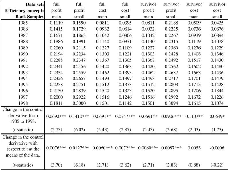
Table 5 shows the control and distance derivatives evaluated at the mean of t and all other exogenous variables. Looking first at the control derivatives ∂NONLEADRANK/∂LEADRANK
|
t=mean for the full data set, we see that all four of these derivatives are all positive and between 0 (no control) and 1 (very good control), as expected. All four are also all statistically significantly different from 0 at the 1% level. The positive, statistically significant control derivatives indicate that after accounting for other factors – such as distance, local market economic conditions, bank and MBHC size, and state regulations – lead bank efficiency and nonlead bankperformance are significantly positively related. This suggests that senior managers at the lead banks are able to transfer their policies, practices, and procedures to management at their nonlead affiliate banks to at least some degree. The control derivatives for profit efficiency rank (.2282 and .2349 for the main sample and small bank sample, respectively) are greater than those for cost efficiency rank (.1362 and .1305, respectively). Because the profit control derivative embodies both cost and revenue control effects, the findings suggest that senior managers may be able exercise some control over both the costs and the revenues of their nonlead affiliate banks. The control over revenues may occur, for example, by influencing the affiliate bank’s service quality, its product mix, the speed and accuracy with which it reprices its loans, its ability to cross-sell new products to existing customers, etc. It is also notable that the control derivatives have similar magnitudes for the main and small bank samples, consistent with little difference in the ability to control nonlead affiliates of different sizes.
The derivatives also appear to be economically significant. For example, the profit efficiency rank coefficient for the main sample of .2282 suggests that a higher profit efficiency rank for the lead bank of 10 percentage points (e.g., from the mean of .4397 to .5397) would yield a predicted increase in the profit efficiency ranks of all its nonlead banks of 2.124 percentage points (e.g., from the sample mean of .6067 to .62794).
Looking next at the control derivatives for the survivor data set in Table 5, all four of these derivatives are positive and statistically significant, and are larger than the corresponding derivatives for the full data set by between 1 and 5 percentage points. These data are again consistent with senior managers at the lead banks exercising some control over nonlead affiliates in terms of both costs and revenues, and suggest that the senior managers of the surviving banks were better able to exercise this control, on average. Again, the results are similar for both the main sample and the small bank sample, suggesting that the senior managers of MBHCs exercise similar amounts of control over nonlead affiliates that are both under and over $100 million in assets.
Although not reported in the tables, the change in the estimated control derivative with respect to distance (i.e., the cross derivative ∂2NONLEADRANK/∂LEADRANK∂lnDISTANCE) was negative and statistically significant in 6 out of the 8 regressions in Tables 3 and 4. This result is consistent with a prior study that found that increased distance interferes with the ability of senior managers to transfer their skills, policies, and practices to affiliate banks (Berger and DeYoung 2001).
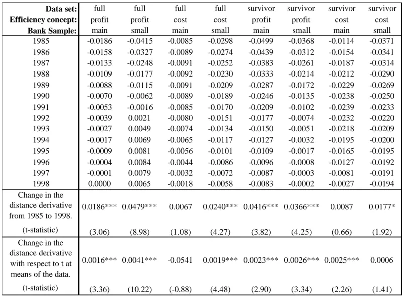
The distance derivatives shown in Table 5, ∂NONLEADRANK/∂lnDISTANCE
|
t=mean, are negative and statistically significant in all eight cases as expected, consistent with our hypothesis greater distance impliesgreater problems in aligning the incentives of local managers with those of the organization, yielding lower profit and cost efficiency. Although the estimated distance derivatives are small in absolute magnitude, around -.02, the effect of a change in distance can be substantial for a banking organization that expands over very large distances within the U.S. For example, the average nonlead bank in the main sample was only about 240 miles away from its headquarters. A doubling of this distance to 480 miles – less than a one standard deviation change in distance and far short of the maximum cross-country distance in the U.S. – would reduce the nonlead bank’s efficiency rank by about 1.4 percentage points (-.02 * ln 2). This is consistent with the existence of nontrivial distance-related agency costs. Note that these estimates may understate the true magnitude of distance-related agency costs due to an “organizational management” effect discussed above.
5.2 Intertemporal Changes in the Control and Distance Derivatives
The main focus of our research is on the changes over time in the control and distance derivatives. As discussed above, the main implications of our hypotheses that improvements in the nonfinancial and financial technologies have improved the control of banking organizations and reduced the agency costs of distance are that the derivatives ∂NONLEADRANK/∂LEADRANK
|
t and ∂NONLEADRANK/∂lnDISTANCE|
t should be increasing with t. We calculate each of these derivatives for the regressions in Tables 3 and 4, and map them over time t in Figures 1 through 4. The year-to-year numbers underlying these figures are displayed in Tables 6 and 7, along with our two formal tests of statistical significance. The second to last row in these tables displays the derivative tests (3) and (6), ∂NONLEADRANK/∂LEADRANK|
t=14 - ∂NONLEADRANK/∂LEADRANK|
t=1 and ∂NONLEADRANK/∂lnDISTANCE|
t=14 - ∂NONLEADRANK/∂lnDISTANCE|
t=1, which measure the change in the control and distance derivatives, respectively, from the beginning to the end of the 1985-1998 sample period. The last row in these tables displays the cross derivative tests (4) and (7),∂2
NONLEADRANK/∂LEADRANK∂t
|
t=mean and ∂2NONLEADRANK/ ∂lnDISTANCE ∂t|
t=mean, which measure the change in the control and distance derivatives, respectively, with respect to time evaluated at the means of the data.We view the profit efficiency results as our principle findings because profit efficiency is superior to cost efficiency for evaluating overall firm performance. We include the cost efficiency results primarily to help to determine whether the effects of technological progress on managing affiliates are reflected primarily in costs versus revenues. We view the derivative tests (3) and (6) as more important, because they measure the effects
of technology over the entire time period, not just at the mean of the data.12
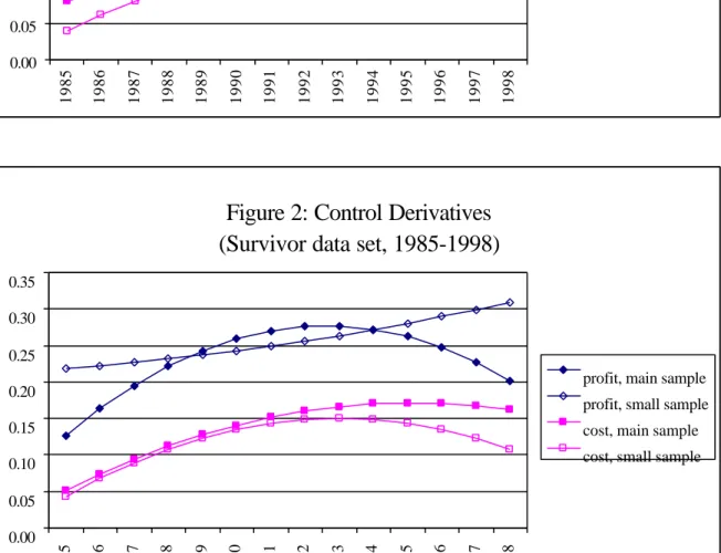
All eight of the control derivatives shown in Figures 1 and 2 are positive and between 0 and 1 for all values of t, as expected. More important, these derivatives are generally increasing over time. In all eight cases, the control derivatives are higher at the end of the sample period than at the beginning, although in some cases the estimated paths decrease somewhat at the end of the sample period. We focus on the change over the entire period from t=1 to t=14, rather than the exact shapes of the curves. The U-shapes and inverted-U-shapes in the figures may reflect the specification of a quadratic functional form. The increases in the profit control derivatives are economically significant, increasing on the order of 50% to 100% over the sample period. For example, in the first column of Table 6 (main sample, survivor data set), the profit control derivative increased by about 60% from .1119 to .1811. The next to last row of Table 6 shows that all eight of the increases in the profit control derivatives are positive and statistically significant, and the last row of Table 6 shows that six of the eight second derivatives with respect to t are positive and statistically significant. Overall, these data are strongly consistent with our hypothesis that technological progress has allowed banking organizations to exercise substantially more control over nonlead affiliates over time.
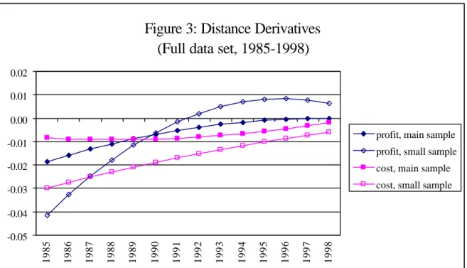
Six of the eight distance derivatives shown in Figures 3 and 4 are negative for all values of t, as expected, although some of the magnitudes are relatively small. The few positive or small negative values for the distance derivatives are consistent with the presence of the “organizational management” effect discussed above. The more important finding is that the distance derivatives are generally increasing over time. All eight of the distance derivatives increase from the beginning to the end of the sample period, and in six of these cases the increase is statistically significant. The increases in the distance derivatives were substantially larger for profit efficiency. These tend to center around .04, suggesting that a doubling of distance from the lead bank would have reduced the profit efficiency rank of a nonlead bank by about 2.8 percentage points less at the end of the sample period than at the beginning (.04 * ln 2). In addition, six of the eight cross derivatives with respect to t (at the means of the data) are positive and statistically different from zero. These data are consistent with our hypothesis that over time, technological progress has reduced the agency costs associated with the distance to the nonlead banks
12
We recognize that the derivatives (3) and (6) are based on fitted regression values far from the means of the data (i.e., at t=1 and t=14); since this reduces the precision of the estimated derivatives, it may be relatively more difficult to reject the null hypothesis in these tests.
in the organization. Furthermore, to the extent that these benefits accrued to banking firms over the sample period, they were likely to be more substantial on the revenue side than on the cost side of the income statement. The intertemporal increases in the control derivatives in Figures 1 and 2, and to a lesser extent the intertemporal increases in the distance derivatives in Figures 3 and 4, occur mostly during the first portion of the sample period. Although the shapes of these estimated time paths are to some extent constrained by the quadratic specification of time, the shapes suggest that improvements in parental control and reductions in the agency costs of distance were easier to achieve during the 1980s and more difficult to achieve during the 1990s. A full investigation of this phenomena is beyond the scope of this study, but we suggest two reasonable hypotheses that are consistent with the data. First, the mergers of the 1990s tended to be larger, more complex, and involve more distant target banks, and as a result may have posed different and more difficult managerial challenges than the mergers of the 1980s. Second, as discussed above, banks may have been able to take early advantage of some of the benefits of technological progress in information processing and telecommunications, consistent with the measured productivity gains made by banks in the late 1980s.
We performed a number of additional robustness checks that are not shown in the tables and figures. We estimated the regressions using subperiods of the data – 1985-1991 (the first half of the panel), 1992-1998 (the second half of the panel), and 1985-1996 (before full effect of Riegle-Neal Act). These regressions yielded results that were qualitatively similar to the results from the full sample period. We also estimated regressions that used efficiency levels rather than efficiency ranks, and used linear distance rather than the natural log of distance. These regressions always produced theoretically correct signs for the control and distance derivatives, although the behavior of these derivatives across time was somewhat less robust. Finally, we replaced the panel regressions with 14 annual cross-section regressions (dropping all of the terms than contain the t variable) which allows all the coefficient estimates to vary by year. The results from the annual regressions were qualitatively similar to those from our panel regressions.
6. Conclusions
The issue of whether technological progress is facilitating the geographic expansion of the banking industry has important implications. Currently, only a few organizations in the U.S. have come close to expanding nationwide or testing the Riegle-Neal cap of 10% of national bank and thrift deposits in one organization, and