The Effects of Monetary-Policy Shocks on Real Wages: A Multi-Country Investigation The Effects of Monetary-Policy Shocks on Real Wages: A Multi-Country Investigationv

The Effects of Monetary-Policy Shocks on Real Wages: A Multi-Country Investigation

Michel Normandin∗

March 2006

Abstract

This paper assesses the plausibility of popular models of the monetary transmis-sion mechanism for the G7 countries. For this purpose, flexible structural vector autoregressions are used to relaxe the restrictions behind the traditional identify-ing schemes of monetary-policy shocks and their effects on macroececonomic vari-ables, and in particular, on real wages. The estimates reveal that expansionary monetary-policy shocks produce declines of real wages for Canada, France, and the United Kingdom. This is consistent with sticky-wage models and suggests that labor-market frictions constitute prime features of these economies. In con-strast, positive monetary-policy shocks yield increases of real wages for Germany, Italy, Japan, and the United States. This is consistent with sticky-price models and limited-participation models, so that goods-market frictions and/or financial-market frictions seem important characteristics of these economies. Finally, the standard identifying restrictions are often statistically rejected and produce severe distortions of real-wage responses.

JEL Classification: C32, E52

Keywords: Conditional Heteroscedasticity; Monetary-Policy Indicators; Orthogo-nality Conditions.

* Mailing address: Department of Economics and CIRP ´EE, HEC Montr´eal, 3000 Chemin de la Cˆote-Ste-Catherine, Montr´eal, Qu´ebec, Canada, H3T 2A7. E-mail address: michel.normandin@hec.ca. Phone number: (514) 340-6841. Fax number: (514) 340-6469. I thank Marcel Aloy, Hafedh Bouakez, and Benoˆıt Mojon for com-ments and Simon Fraser for research assistance. I acknowledge financial support from the Fonds Queb´ecois de la Recherche sur la Soci´et´e et la Culture (FQRSC) and Social Science and Humanities Research Council of Canada (SSHRC).

1. Introduction

Monetary policies are at the center of several ongoing economic debates, such as selections of exchange rate regimes, determinations of monetary zones, and con-trols of inflation costs. In this context, it is important to understand the effects of monetary policies on key macroeconomic variables. This has motivated the de-velopment of several models of the monetary transmission mechanism. Recently, substantial attention has been devoted to sticky-wage models, sticky-price models, and limited-participation models. Sticky-wage models incorporate frictions on the labor market by stipulating that firms do not adjust intantaneously nominal wages (e.g. Ascari 2000; B´enassy 1995; Bordo, Erceg, and Evans 2000). Sticky-price mod-els include frictions on the goods market by postulating that firms do not adjust immediately prices (e.g. Chari, Kehoe, and McGrattan 2000; Rotemberg 1996; Yun 1996). Limited-participation models involve frictions on the financial market by assuming that households do not adjust instantaneously their portfolio choices (e.g. Christiano and Eichenbaum 1995; Fuerst 1992; Lucas 1990).

Designing models which incorporate the various classes of frictions just de-scribed proves useful to explain a substantial portion of the cyclical fluctuations of the U.S. economy (e.g. Christiano, Eichenbaum, and Evans 2005). Yet, con-fronting models which isolate the different types of frictions proves useful to gauge the relative importance of the labor-market frictions, goods-market frictions, and financial-market frictions (e.g. Christiano, Eichenbaum, and Evans 1997). Such ex-ercise reveals the prime features of the structure of the economy of a country. This information is important to elaborate several global and country-specific macroeco-nomic policies, and in particular, monetary policies.

It is attractive to assess the relative importance of the various frictions from the empirical dynamic effects of expansionary monetary-policy shocks, given that the alternative models lead to different predictions following such policies. Namely, the decrease of interest rate and increases of output and prices are predicted to be of different magnitudes and persistences across models. For example, prices increase instantaneously in sticky-wage models and limited-participation models, whereas they increase fairly slowly in sticky-price models. Unfortunately, it becomes most challenging to use these price responses to detect the prime frictions, since no clean-cut criterion exists to evaluate the adjustment rapidity of a variable. However, the inertia in nominal wages implies that real wages decline in sticky-wage models, while they increase in sticky-price models and limited-participation models. Thus, it is possible to use these real-wage responses to determine, at least, the importance of labor-market frictions relative to goods-market frictions and financial-market frictions, based on the strict creterion of the sign of real wage responses.

In this spirit, structural vector autoregressions (SVAR) are specified to iden-tify monetary-policy shocks and measure their effects on macroececonomic variables, and in particular, on real wages. Empirically, some SVAR analyses indirectly con-clude, from the relative magnitudes of nominal-wage responses and price responses, that expansionary monetary-policy shocks lead to temporary declines of real wages for synthetic euro-area data, but to transient increases of real wages for Germany and the United States (Peersman and Smets 2001; Sims 1980; Sims and Zha 1998). Other SVAR analyses directly show that real-wage responses are positive for the United States (Christiano, Eichenbaum, and Evans 1997). This latter result is ro-bust to economy-wide and sector-specific measures of real wages and to standard identification schemes of monetary-policy shocks.

Typically, the identification schemes impose various targeting and orthogo-nality restrictions. The targeting restrictions define the monetary authority’s policy indicator. The orthogonality restrictions may state that the monetary authority’s exogenous policy actions have no impact effects on certain macroeconomic variables such as output, prices, and real wages. Alternatively, the orthogonality restrictions may assume the inexistence of monetary authority’s endogenous policy adjustments to changes in macroeconomic variables. These restrictions usually lead to exact identification, and thus, are unfortunately untestable.

This paper attempts to improve on earlier work by relaxing and testing the standard identifying restrictions. This exercise relies on a flexible SVAR that dis-plays three important features (Normandin and Phaneuf 2004). First, it relaxes the traditional assumption that structural innovations are conditionally homoscedastic. Importantly, time-varying conditional volatilities may lead to over identification, so that the typical restrictions become testable (Sentana and Fiorentini 2001). Sec-ond, our SVAR incorporates a simple formulation of the monetary market, which nests two popular monetary-policy indicators. Thus, the validity of the restrictions associated with interest-rate targeting (e.g. Bernanke and Blinder 1992; Chris-tiano, Eichenbaum, and Evans 1997; Sims 1992) and monetary-aggregate targeting (e.g. Christiano and Eichenbaum 1992; Eichenbaum 1992; Sims 1980) can be ver-ified. Third, our SVAR admits current interactions between the monetary-policy variables and the other macroeconomic variables. Hence, the validity of the or-thogonality restrictions related to the absence of impact effects of exogenous policy actions (e.g. Christiano and Eichenbaum 1992; Eichenbaum 1992) and the inexis-tence of endogenous policy adjustments (e.g. Sims 1980, 1992) can be checked.

using monthly data for the post-1983 period. The estimates are used to recover the structural innovations, and in particular, the measures of policy shocks in order to document the monetary authorities’ exogenous actions. Importantly, at least all, but one, structural innovations display time-varying conditional variances for all countries. Also, the policy-shock measures exhibit conditional volatilities which are constant for Canada and the United Kingdom, moderately persistent for Germany, Italy, and Japan, and very persistent for France and the United States. Moreover, the policy-shock measures are consistent with exogenous domestic policy actions (rather than endogenous adjustments to foreign-country phenomena), since they are not statistically correlated for all pairs of countries. Finally, the policy-shock measures are always consistent with the common observation of monetary analysts that policy actions tend to be tight in expansionary phases and loose during con-tractionary periods.

The estimates of the flexible SVAR are further used to compute the dynamic responses in order to assess the effects of unanticipated expansionary monetary poli-cies on marcroeconomic variables. Empirically, such shocks lead to the decrease of interest rate and increases of monetary aggregate, output, and prices. This accords with sticky-wage models, sticky-price models, and limited-participation models. Also, positive monetary-policy shocks produce declines of real wages for Canada, France, and the United Kingdom. This is consistent with sticky-wage models and suggests that labor-market frictions constitute prime features of these economies. In constrast, positive monetary-policy shocks yield increases of real wages for Ger-many, Italy, Japan, and the United States. This is consistent with sticky-price models and limited-participation models, so that goods-market frictions and/or financial-market frictions seem important characteristics of these economies.

The various identifying schemes associated with standard targeting and or-thogonality restrictions are next tested. Empirically, the restriction behind monetary-aggregate targeting cannot be statistically rejected for all countries, ex-cept France. In contrast, the restriction related to interest-rate targeting is refuted for all countries, but France. Also, the orthogonality restrictions imposing that the monetary authority’s exogenous policy actions have no impact effects on macroe-conomic variables are rejected for all countries, except the United States. Finally, the alternative orthogonality restrictions stipulating the inexistence of monetary authority’s endogenous policy adjustments are refuted for all countries, but France and the United States.

For completeness, the economic consequences of imposing statistically in-valid restrictions are verified. Such restrictions often produce severe distortions of the policy-shock measures: they display incorrect signs, and thus, lead to er-roneous indications about the direction of the exogenous policy actions for most countries. Moreover, the invalid restrictions frequently yield pronounced distor-tions of the real-wage responses: they display incorrect signs, and thus, lead to erroneous selections about models of the monetary transmission mechanism for many countries. For example, imposing false restrictions often incorrectly suggests the relevance of sticky-price models or limited-participation models for Canada, France, and the United Kingdom, and sticky-wage models for Germany and Japan. However, placing invalid restrictions does not alter the conclusions regarding the monetary transmission mechanism for Italy and the United States.

The paper is organized as follows. Section 2 presents our flexible SVAR specification. Section 3 outlines the estimation strategy and the underlying identifi-cation conditions. Section 4 estimates the SVAR parameters and tests the standard

targeting and orthogonality restrictions. Sections 5 and 6 analyze the consequences of the various restrictions for monetary-policy measures and their dynamic effects. Section 7 concludes.

2. Specification

Throughout our analysis, a flexible SVAR system is used for each country to identify monetary-policy shocks and estimate their effects on macroeconomic variables. The system expresses the contemporaneous interactions between the variables, in innovation form, as follows:

Aνt =t. (1)

The vector νt contains the statistical innovations extracted from the observed

macroeconomic variables. The vector t includes the unobserved structural

inno-vations. The matrix A measures the interactions between current statistical inno-vations. The matrix B = A−1 measures the impact responses of the variables to the structural innovations. The dynamic responses of the variables are obtained by substituting the impact responses into the VAR.

A distinction is established between variables which are outside the monetary market or non-monetary variables, and variables that belong to the monetary mar-ket or monetary variables. The non-monetary variables are output, yt, aggregate

prices, pt, commodity prices, ct, and real wages, wt. The monetary variables are

the monetary aggregate,mt, and short-term interest rate,rt. Except for real wages,

this set of variables is often used in multi-country studies based on SVAR systems (e.g. Kim 1999; Sims 1992). To achieve our goal, real wages are also included to

assess their responses following monetary-policy shocks.

The monetary market is further developed by considering the simple formu-lation:

νms_,t =φσ_dd,t+σ_ss,t, (2.1)

νmd_,t =−αν_r,t+σ_dd,t. (2.2)

The terms νms_,t and ν_md_,t denote the statistical innovations of the money

sup-ply and money demand. The structural innovations s,t and d,t correspond to

monetary-policy shocks and money-demand shocks. The parameters σs and σd are

the standard deviations scaling the structural innovations of interest, the coefficient

αis constrained to be positive, and the parameter φis unrestricted. Equation (2.1) describes the procedures which may be used by the monetary authority to select its policy instruments. Equation (2.2) represents the demand for money, in innovation form.

The equilibrium solution of the monetary market (2) is inserted in the SVAR (1) to yield:        a11 a12 a13 a14 a15 a16 a21 a22 a23 a24 a25 a26 a31 a32 a33 a34 a35 a36 a41 a42 a43 a44 a45 a46 a51 a52 a53 a54 (1−φ)/σs −(φα)/σs a61 a62 a63 a64 1/σd α/σb               νy,t νp,t νc,t νw,t νm,t νr,t        =        1,t 2,t 3,t 4,t s,t d,t        . (3)

For conciseness, Ann = [aij] (where i = 1, . . . ,4 and j = 1, . . . ,4) defines the

Amm= [aij] (where i= 5,6 andj = 5,6) corresponds to the constrained, but

non-zero, coefficients related to the block of monetary variables. Anm = [aij] (where

i = 1, . . . ,4 and j = 5,6) and Amn = [aij] (where i = 5,6 and j = 1, . . . ,4)

represent the unconstrained parameters across the blocks of variables. Thus, the system (3) allows for interactions between the terms within and across the blocks of non-monetary and monetary variables. As a result, all non-monetary and monetary variables may contemporaneously be affected by the structural innovations, and in particular, by monetary-policy shocks.

To gain intuition, the fifth equation of system (3) is rewritten as:

νs,t=

h

ρ51νy,t+ρ52νp,t+ρ53νc,t+ρ54νw,t

i

+σss,t. (4)

Equation (4) is interpreted as the monetary authority’s feedback rule. The term

νs,t = (1 − φ)νm,t −(αφ)νr,t

corresponds to the statistical innovation of the monetary-policy indicator. This indicator exclusively involves the monetary vari-ables, since they convey information about the stance of monetary policy. In general, the indicator reveals that the monetary authority adopts a mixed procedure where it neither pursues pure interest-rate targeting (φ 6= 1) nor strict monetary-aggregate targeting (φ 6= 0). The expression between brackets in (4) captures the system-atic responses of the monetary authority to changes in non-monetary variables. In general, these feedback effects occur because the monetary authority designs its policy by taking into account the current values of each non-monetary variables (ρ5j =−a5jσs 6= 0 for j = 1, . . . ,4). Moreover, the term (σss,t) represents scaled

monetary-policy shocks. These shocks capture exogenous policy actions taken by the monetary authority.

Also, the conditional-scedastic structure of system (3) is given by:

AΣtA0 = Γt. (5)

Here, Σt = Et−1(νtνt0) represents the conditional non-diagonal covariance matrix

of the non-orthogonal statistical innovations. Γt = Et−1(t0t) is the conditional

diagonal covariance matrix of the orthogonal structural innovations. I = E(t0t)

normalizes (without loss of generality) the unconditional variances of the structural innovations to unity. The conventional studies impose Γt =I, so that the structural

innovations are conditionally homoscedastic. This implies Σt =BB0, such that the

conditional second moments of the statistical innovations are time-invariant. In contrast, our analysis relies on Γt 6= I, which allows conditional heteroscedasticity

of the structural innovations. As a result, Σt 6= BB0, which permits time-varying

conditional second moments of the statistical innovations.

Finally, the dynamics of the conditional variances of the structural innova-tions is specified as:

Γt = (I−∆1−∆2) + ∆1•(t−10t−1) + ∆2•Γt−1. (6)

The operator • denotes the element-by-element matrix multiplication, while ∆1 and ∆2 are diagonal matrices of parameters. Equation (6) characterizes the con-ditional variances of the structural innovations from univariate generalized autore-gressive conditional heteroscedastic [GARCH(1,1)] processes, where ∆1 contains the ARCH coefficients and ∆2 incorporates the GARCH coefficients. In general, the GARCH(1,1) processes offer the considerable advantages of being more parsi-monious than alternative large-scale multivariate specifications (e.g. Diebold and

Nerlove 1989; Normandin and St-Amour 1998) and of reproducing alternate periods of volatility and smoothness which characterize several macroeconomic time-series (e.g. Bollerslev, Chou, and Kroner 1992; Pagan and Robertson 1995). In our case, positive definite ∆1, ∆2, and (I−∆1−∆2) imply that all structural innova-tions display time-varying (positive and stationary) conditional variances. Positive semi-definite ∆1 and ∆2, and positive definite (I−∆1−∆2) signify that only some structural innovations exhibit conditional heteroscedasticity. Zero ∆1and ∆2 imply that all structural innovations are conditionally homoscedastic. Also, the intercepts (I−∆1−∆2) are consistent with the normalization I =E(t0t).

3. Estimation Strategy

The estimation of the specification just presented is performed by resort-ing to a two-step procedure which explicitly takes into account the conditional heteroscedasticity and orthogonality of the structural innovations (Normandin and Phaneuf 2004). The first step consists in an equation-by-equation ordinary least squares (OLS) estimation of the coefficients of a τ-order VAR process. From this exercise, the estimates of the statistical innovations νt and of their conditional

co-variances Σt are recovered fort = (τ + 1), . . . , T. Specifically, the estimate of Σt is

computed by using equations (5) and (6) evaluated for system (3), by initializing Γτ = (τ0τ) = I from the unconditional moments, and by giving values to the

pa-rameters Θ — where Θ is the vector composed of all the non-zero elements of A, ∆1, and ∆2.

The second step is a maximum-likelihood (ML) estimation of the parameters included in Θ. The log-likelihood of the sample (ignoring the constant term) is constructed by assuming that the statistical innovations are conditionally Gaussian:

L(ν,Θ) =−1 2 T X t=τ+1 log|Στ| − 1 2 T X t=τ+1 ν_t0Σ−_t 1νt, (7)

where νt and Σt are evaluated at their estimates. The log-likelihood (7) is then

maximized over the parameters Θ using the BHHH algorithm.

The importance of exploiting the conditional heteroscedasticity and orthog-onality of the structural innovations is highlighted by considering the alternative system:

A∗νt =∗t, (8)

whereA∗ =QA,∗_t =Qt, and Q is an arbitrary orthogonal transformation matrix

(i.e. QQ0 = Q0Q = I). Clearly, system (3) is econometrically identified when A is unique (up to column sign changes) under orthogonal transformations, soQ= Iand

Q=I1/2_{are the only admissible transformations preserving the orthogonality of the} rotated structural innovations in (8) (i.e. Γ∗_t =QΓtQ0 is diagonal). Moreover, fixing

the sign of the diagonal elements of A ensures global identification. This implies that monetary-policy shocks are identified. This also means that B is uniquely defined and the effects of monetary-policy shocks are identified. In practice, this translates into a log-likelihood function (7) that is not flat. That is, system (3) yields similar estimates of the parameters under alternative starting values for Θ.

The sufficient (rank) condition for identification states that the conditional variances of the structural innovations are linearly independent. That is, λ = 0 is the only solution to Γλ = 0, such that (Γ0Γ) is invertible — where Γ stacks by column the conditional volatilities (for t = (τ + 1), . . . , T) associated with each

structural innovation. The necessary (order) condition requires that the conditional variances of (at least) all, but one, structural innovations are time-varying. In practice, the rank and order conditions lead to similar conclusions, given that the conditional variances are parametrized by GARCH(1,1) processes (Sentana and Fiorentini 2001).

Unlike our estimation procedure, the conventional studies based on SVAR systems impose the conditional homoscedasticity of all structural innovations. In this context, systems (3) and (8) are observationally equivalent up to second mo-ments (i.e. Σ∗_t = Σt = BB0) with orthogonally rotated structural innovations (i.e.

Γ∗_t = QΓtQ0 = I is diagonal) for any admissible transformation matrices Q. It

follows that A and B are not unique, so monetary-policy shocks and their effects on macroeconomic variables are not identified. In practice, this translates into a log-likelihood function (7) that is flat.

In this context, a common strategy is to identify the monetary-policy shocks without having to identify the entire system (3). To do so, it is sufficient, for example, to impose two types of restrictions which ensure , first, the identification of the monetary block Amm and, second, the zero conditions Anm = 0. In such a

case, Am = (A0nm|A

0

mm)

0 _{= (0}0_|A0

mm)

0 _{is uniquely determined (up to column sign}

changes), so that Qnm = 0 and Qmm = I or Qmm = I1/2 are the only admissble

submatrices. Moreover, fixing the sign of the diagonal elements ofAmm guarantees

that monetary-policy shocks are globally identified. Hence, Bm = (Bnm0 |B

0

mm)

0

= (00|A−_mm1 0)0is also unique, so that the effects of monetary-policy shocks are identified.

First, the exact identification of Amm can be achieved by imposing a

and three distinct time-invariant covariances. From an economic perspective, this restriction defines the monetary-policy indicator as follows.

R Indicator: φ= 1. The monetary-policy indicator in the feedback rule (4) reduces

toνs,t=−ανr,t, so that the interest rate is the single policy variable (e.g. Bernanke

and Blinder 1992; Christiano, Eichenbaum, and Evans 1997; Sims 1992). In this context, changes in the interest rate entirely summarize the stance of the monetary policy. This is because the monetary authority targets the interest rate by fully offseting money-demand shocks.

M Indicator: φ = 0. The monetary-policy indicator in (4) becomes νs,t = νm,t,

such that the monetary aggregate is the single policy variable (e.g. Christiano and Eichenbaum 1992; Eichenbaum 1992; Sims 1980). Therefore, changes in the monetary aggregate completely reveal the stance of the policy. This occurs because the authority targets the monetary aggregate, and as such does not respond at all to money-demand shocks.

Second, the economic interpretation of the zero conditions Anm = 0 is the

following.

No-Impact Effects: Anm = 0. The monetary-policy shocks have no impact effects

on the non-monetary variables (e.g. Christiano and Eichenbaum 1992; Eichenbaum 1992). This implies that monetary-policy shocks are orthogonal to the variables involved in the systematic component of the feedback rule (4). In addition, the ab-sence of impact effects occurs because monetary-policy shocks have no direct effects and indirect effects. The direct effects correspond to the contemporaneous responses of the non-monetary variables to the policy variable. Thus, these effects are cap-tured by the coefficients ai5 andai6 (wherei= 1, . . . ,4) under the M Indicatorand

R Indicator, respectively. The indirect effects correspond to the contemporaneous effects of the policy variable on the non-monetary variables through its current im-pact on the non-policy monetary variable. Hence, these effects are reflected by ai6 and ai5 (where i= 1, . . . ,4) under the M Indicator and R Indicator.

In practice, this identification scheme is implemented by measuring monetary-policy shocks from Choleski decompositions of the VAR-residual covari-ance matrix, which imply that Ais lower triangular with positive elements on the diagonal. These decompositions are obtained by ordering the non-monetary vari-ables first, followed by the policy variable, and by the other monetary variable. Note that the measure of monetary-policy shocks are not altered by the particular ordering within the block of non-monetary variables, since the system is not entirely identified. Also, the associated restrictions defining the monetary-policy indicator and ruling out the impact effects are untestable, given that the system is not entirely identified.

Alternatively, the identification of monetary-policy shocks can be achieved by imposing restrictions which ensure the identification of the monetary blockAmm

and the zero conditions Amn = 0, rather than Anm = 0. Some implications of the

alternative zero conditions are the following.

No-Feedback Effects: a5j = 0 (where j = 1, . . . ,4). There is no systematic

compo-nent in the feedback rule (4) since ρ5j = 0 (e.g. Sims 1980, 1992). This implies

that the monetary authority does not adjust endogenously the policy to respond to current non-monetary phenomena.

In practice, this alternative identification scheme is implemented from Choleski decompositions obtained by ordering the policy variable first. Again, the

particular ordering of the non-policy variables is irrelevant and the underlying re-strictions are untestable.

4. Estimation Results

The estimation results are obtained from monthly data for the G7 countries. The sample covers the 1983-01 to 1998-12 period for France, Germany, and Italy, and the 1983-01 to 2001-10 period for Canada, Japan, the United Kingdom, and the United States. Germany refers to West Germany and Unified Germany for the pre- and post-1990 periods. According to many observers, the post-1983 period represents a fairly stable economic environment for many of the G7 countries. In principle, this eases the identification of monetary-policy shocks, since the associated measures are less likely to be contaminated by major non-monetary phenomena (e.g. oil shocks). Also, the pre-1999 period for France, Germany, and Italy focuses on the episode before the European Monetary Union. As usual, the series are at the monthly frequency. Compared to lower frequency data, these series are likely to display greater conditional volatilities, which constitute a crucial feature for our estimation strategy.

The variables involved in system (3) are mostly measured from the Interna-tional Financial Statistics (IFS) released by the InternaInterna-tional Monetary Funds and the Main Economic Indicators (MEI) published by the Organization for Economic Cooperation and Development. The non-monetary variables are computed as fol-lows. As is standard practice, yt corresponds to the industrial-production indices

(source: IFS) and pt is the consumer-price indices (source: IFS) for all countries.

Also, ct is measured as the world-export commodity-price index in U.S. dollars

currencies by using the market exchange rate (source: IFS) for the other countries. This variable captures inflationary pressures and foreign-economic changes reflected in exchange-rate movements (Sims 1992; Kim 1999). Finally,wt is computed as the

nominal wages (source: MEI) normalized by pt. The nominal wages correspond

to the (hourly, weekly, or monthly) earning indices of the manufacturing sector for Canada, Germany, Japan, the United Kingdom, and the United States. The nom-inal wages are captured by the (hourly) wage rates of the industry sector for Italy and of all activities for France. The nominal wages are interpolated from quarterly to monthly frequencies (source: DISTRIB procedure in RATS) for France and Ger-many. These measures of nominal wages are mainly dictated by the availability of the data. An obvious exception is that both sector-specific and economy-wide mea-sures of nominal wages are reported for the United States. Given that the various measures of nominal wages for the United States yield similar effects of monetary-policy shocks (Christiano, Eichenbaum, and Evans 1997), our analysis relies on the manufacturing-sector data to facilitate comparisons with most of the G7 countries.

The monetary variables are computed as follows. The variablert is measured

by the overnight money-market rate (source: MEI) for Canada, the call-money rates (source: IFS) for France, Germany and Japan, the mid-term government-bond yield (source: IFS) for Italy, the minimum overnight interbank rate (source: IFS) for the United Kingdom, and the Federal-funds rate (source: IFS) for the United States. These measures are similar to the data often used in previous multi-country studies (e.g. Kim 1999; Sims 1992). Also,mt corresponds to M1 (source: MEI) for France

and (source: IFS) for Canada, Germany, Italy, and Japan, but to Retail M4 (source: Bank of England) for the United Kingdom and M2 (source: Federal Reserve Bank of St-Louis macro database - Fred) for the United States. M1 is selected for most

countries since it is frequently used in earlier multi-country analyses (e.g. Sims 1980, 1992). Retail M4 for the United Kingdom is dictated by the availability of the data and is close to the definition of M2. Finally, M2 is selected for the United States to conform with previous SVAR analyses evaluating the effects of monetary-policy shocks on real wages for this country (e.g. Christiano, Eichenbaum, and Evans 1997; Sims and Zha 1998).

The non-monetary and monetary variables are all expressed in logarithms, except the short-term interest rates. The variables are further measured from seasonally-adjusted data, whenever possible. For each country, these variables are used to calculate the OLS estimates associated with a VAR process which includes a complete set of seasonal dummies and six lags (τ = 6). For all cases, the Ljung-Box and heteroscedastic-robust Lagrange-Multiplier (LM) test statistics are never significant (at the 5% level) for p-order autocorrelations and AR(p) processes of the VAR residuals (with p = 1,3, and 6). In contrast, the McLeod and LM test statistics are sometimes significant forp-order autocorrelations of the squared VAR residuals and ARCH(p) effects (with p = 1,3, and 6). These findings suggest the presence of conditional heteroscedasticity in some statistical innovations, which is likely to translate into time-varying conditional variances of structural innovations — given that Σt 6=BB0 if Γt 6=I.

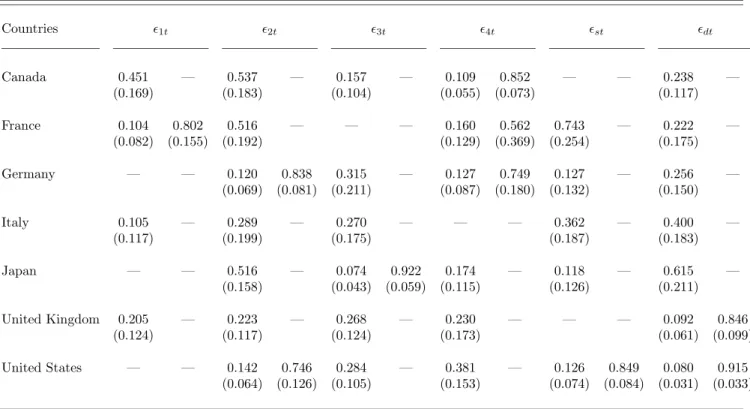
For briefness, the ML estimates are only reported for the GARCH(1,1) co-efficients, the monetary-market parameters, as well as the impact and feedback effects. Table 1 presents the estimates of the GARCH(1,1) parameters. For each country, the estimates imply that (I −∆1 −∆2) is positive definite, whereas ∆1 and ∆2 are positive semi-definite since all, but one, structural innovations display time-varying conditional volatilities. This accords with the order condition for the

identification of system (3). Also, (Γ0Γ) has a large positive determinant and is in-vertible. This is consistent with the rank condition. Overall, these findings confirm that monetary-policy shocks and their effects are identified.

For all countries, the McLeod and LM test statistics are never significant for p-order autocorrelations of the squared structural innovations (relative to their conditional variances) and GARCH(p,q) effects (with p = 1,3, and 6 and q = 1). This suggests that the estimates of the GARCH(1,1) coefficients provide an ade-quate description of the conditional heteroscedasticity of all structural innovations, and in particular, of monetary-policy shocks. In addition, monetary-policy shocks exhibit conditional volatilities which are constant for Canada and the United King-dom, moderately persistent for Germany, Italy, and Japan, and very persistent for France and the United States — where the persistence is measured by the sum of the ARCH and GARCH coefficients.

Table 2 shows the estimates of the monetary-market parameters. For all countries, the estimates exhibit the expected signs, although there are often impre-cise. The estimates ofσs andσd reveal that the sizes of monetary-policy shocks are

always numerically smaller than those of the money-demand shocks. The estimates of α indicate that the slope of the money demand is systematically negative, and is statistically significant for Italy, Japan, and the United States. The estimates of

φ are not significantly different than zero for all countries, except France. Further-more, the estimates of φ are statistically different than one for all countries, but France. Thus, these results support the restriction associated with the M Indicator

for Canada, Germany, Italy, Japan, the United Kingdom, and the United States, and the restriction behind the R Indicatorfor France.

Table 3 displays the estimates of the impact effects. The estimates of ai5

(for i = 1, . . . ,4) are jointly significant for all countries, except France and the

United States. Also, the estimates of ai6 (for i = 1, . . . ,4) are jointly significant for Canada, France, Japan, and the United Kingdom. Given the definition of the policy variable for each country, these results suggest that monetary-policy shocks have direct effects for Canada, France, Germany, Italy, Japan, and the United Kingdom. Specifically, the estimates of the individual coefficients indicate that these direct effects are significant on aggregate prices for Canada, France, and Germany, commodity prices for Italy, output for the United Kingdom, as well as output, commodity prices, and real wages for Japan. In addition, monetary-policy shocks have indirect effects for Canada, Japan, and the United Kingdom. The estimates of the individual coefficients reveal that these indirect effects are significant on output for Canada, real wages for the United Kingdom, and output and commodity prices for Japan. In sum, the results suggest that the restrictions related to the

No-Impact Effectsare rejected for Canada, France, Germany, Italy, Japan, and the

United Kingdom, but not for the United States.

Table 4 reports the estimates of the feedback effects. The estimates of a5j

(for j = 1, . . . ,4) are jointly significant for all countries, except France and the

United States. In addition, the estimates of the individual coefficients suggest that the monetary authority adjusts endogenously the policy to current movements in aggregate prices for Canada, commodity prices for Italy and Japan, as well as output and real wages for the United Kingdom. Thus, the results reject the restrictions associated with the No-Feedback Effects for Canada, Germany, Italy, Japan, and the United Kingdom, but not for France and the United States.

ade-quately recovered from Choleski decompositions for most countries. This occurs because the zero conditions associated with both the No-Impact Effects and

No-Feedback Effects are rejected for Canada, Germany, Italy, Japan, and the United

Kingdom. In contrast, the findings indicate that Choleski decompositions obtained by ordering the interest rate first should be valid for France, given that the re-strictions behind the R indicator and No-Feedback Effects are not refuted. Finally, Choleski decompositions obtained by ordering the monetary aggregate either first or after the non-monetary variables should be relevant for the United States, since the restrictions related to the M indicator, No-Impact Effects, and No-Feedback Effects

are not rejected.

5. Monetary-Policy Measures

The unrestricted monetary-policy measures are extracted from the flexible conditional-heteroscedastic SVAR (3). This system captures the impact effects (Anm 6= 0) and feedback effects (Amn 6= 0). Also, the associated feedback rule

(4) implies a policy indicator involving both the interest rate (φ6= 0) and monetary aggregate (φ 6= 1), a systematic component (ρ5j 6= 0 for j = 1, . . . ,4), and policy

shocks.

Empirically, the unrestricted measures of the systematic component are sig-nificantly correlated for almost all pairs of countries. This suggests that the sys-tematic components reflect endogenous reactions to foreign variables, and perhaps, to foreign monetary policies. In particular, the strong correlations between the sys-tematic components for the various countries and for the United States may capture the endogenous adjustments of these countries to the U.S. monetary policy. Like-wise, the significant correlations between the systematic components for France or

Italy and for Germany may reflect the endogenous adjustments of the European Monetary System members to the German monetary policy. Note that these strong correlations occur even if the feedback rule (4) does not explicitly include foreign monetary variables (e.g. Grilli and Roubini 1995; Kim and Roubini 2000). However, the correlations arise because the U.S. and German monetary policies presumably affect the exchange rates (used to convert commodity prices in national currencies) of most countries and potentially jointly alter domestic and foreign outputs, prices, or real wages. Finally, the unrestricted measures of monetary-policy shocks are not statistically correlated for all pairs of countries. This suggests that our iden-tified monetary-policy shocks reflect the exogenous policy actions occuring in each country.

Figure 1 plots the smoothed unrestricted measures of monetary-policy shocks. For ease of interpretation, the measures smooth the noisy (serially uncorre-lated) monetary-policy shocks from a five-month centered, equal-weighted moving average. Also, negative (positive) values of the smoothed measures reflect contrac-tionary (expansionary) monetary-policy shocks. Empirically, the unrestricted mea-sures are generally consistent with common observations about changes in monetary policy occuring through the business-cycle phases. That is, the monetary-policy ac-tions tend to be tight in expansionary phases and loose in contractionary periods, so that monetary-policy shocks typically display countercyclical movements. For example, the monetary-policy actions are tight at the business-cycle peaks, loose during the contractionary phases, and tight slightly before the troughs for Canada, Japan, and the United Kingdom. Also, the monetary-policy actions are loose just after the peaks and before the troughs for France, Germany, Italy, and the United States.

Figure 1 also confronts the smoothed unrestricted and restricted measures of monetary-policy shocks. The restricted measures are extracted from conditional-heteroscedastic systems which impose the restrictions associated with either the

M Indicator, R Indicator, No-Impact Effects, or No-Feedback Effects. Empirically,

the unrestricted and restricted measures are similar for most countries, as long as the associated restrictions are statistically valid. In contrast, the unrestricted and restricted measures substantially deviate for many cases, when the associated re-strictions are significantly rejected. The distortions are particularly severe under the restrictions related to the M Indicator for France, the R Indicator for Canada, Germany, Italy, the United Kingdom, and the United States, theNo-Impact Effects

for Canada, Japan, and the United Kingdom, as well as the No-Feedback Effects

for Japan and the United Kingdom. For these cases, the restricted measures of monetary-policy shocks frequently display incorrect magnitudes and signs, and as such indicate incorrect amplitudes and directions of the policy actions. Overall, these results suggest that imposing invalid restrictions can lead to important mis-measurements of monetary-policy shocks.

6. Dynamic Responses

The unrestricted dynamic responses are computed from the flexible conditional-heteroscedastic SVAR (3), which captures the impact effects (Anm6= 0)

and feedback effects (Amn 6= 0), as well as policy indicators involving both the

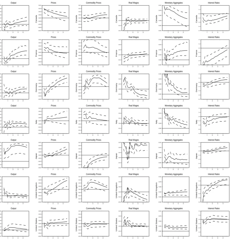
in-terest rate (φ6= 0) and monetary aggregate (φ6= 1). Figure 2 displays the dynamic responses of the various variables following positive, one unconditional standard-deviation, monetary-policy shocks. This figure also shows the (possibly asymetric) 68% probability intervals computed from a bayesian procedure (Sims and Zha 1999).

For the monetary variables, the effects of policy shocks are the following. First, the monetary-aggregate responses are statistically significant, highly persis-tent, and positive for all countries. For example, these responses smoothly decline over the horizons for Canada, Germany, and Italy, are fairly stable for Japan, the United Kingdom, and the United States, and gradually increase for France.

Second, the interest-rate responses are always statistically negative at im-pact. However, these responses display different magnitudes and persistences across countries. That is, they are pronounced for Canada, France, and the United King-dom, compared to those for Germany, Italy, Japan, and the United States. This occurs because the declines of interest rate are reversed less rapidly for the coun-tries where the inflationary pressures from monetary expansions tend to be less persistent, as will be discussed below. Importantly, such transient liquidity effects are predicted by most mainstream macroeconomic theories, including sticky-wage models, sticky-price models, and limited-participation models. In addition, the sys-tematic impact decreases of interest rate and increases of monetary aggregate lead to contemporaneous increases of the monetary-policy indicators, which confirm a loose monetary policy stance.

For the non-monetary variables, the effects of policy shocks are the following. First, the output responses are always positive over some horizons and statistically significant for all countries, but Canada. In addition, these responses are hump-shaped so that the increase in economic activity is followed by a return to the intitial level for all countries, except the United Kingdom. These findings provide empirical support for macroeconomic theories predicting the non-neutrality of money, such as sticky-wage models, sticky-price models, and limited-participation models.

Second, the price responses are positive for most horizons and are generally statistically significant. This accords with mainstream macroeconomic theories, which predict that inflationary pressures are exerted by monetary expansions. Also, prices increase drastically at impact and then decline smoothly for Canada and France. This pattern seems consistent with sticky-wage and limited-participation models, where price adjustments are instantaneous. Prices adjust fairly slowly by increasing only after around six months for Germany, Japan, the United Kingdom, and the United States. This pattern seems to accord with sticky-price models, which predict a significant amount of inertia in aggregate-price behavior. Prices exhibit almost no reaction at impact, but then increase relatively quickly for Italy. This pattern is not entirely consistent with neither sticky-wage models, sticky-price models, nor limited-participation models. It further illustrates that model selections based on price behavior are challenging, since no formal criterion exists to determine the rapidity of price adjustments.

Third, the commodity-price responses are positive over some horizons for Canada, France, Germany, Italy, and the United Kingdom, are fairly stable for the United States, and are largely negative for Japan. In principal, these responses can either be negative, null, or positive. This is explained, in part, by the behavior of exchange rates (used to convert commodity prices in national currencies). That is, the national currencies may appreciate or depreciate at impact depending on the revisions of expected inflation following monetary expansions.

Fourth, the real-wage responses are transient for most countries, but are very persistent for Japan and the United Kingdom. Moreover, the real-wage responses are statistically negative for Canada, France, and the United Kingdom. This pattern is consistent with a substantial degree of inertia in nominal wages as predicted

by sticky-wage models, and suggests that labor-market frictions constitute prime features of these economies. In contrast, the real-wage responses are significantly positive for Germany, Italy, Japan, and the United States. This pattern accords with instantaneous adjustments of nominal wages as implied by sticky-price models and limited-participation models, and suggests that goods-market frictions and/or financial-market frictions are important characteristics of these economies. Also, these findings corroborate previous results documented for Germany and the United States. Finally, recall that model selections based on real-wage behavior rely on a strict creterion, namely the sign of the real-wage responses. In this sense, such model selections are less controversial than those based on price behavior.

For completeness, the consequences of imposing the various restrictions on the dynamic responses are evaluated. This exercise is performed exclusively for the real-wage responses in order to invoke our strict creterion of model selections. Figure 3 compares the unrestricted and restricted dynamic responses of real wages to expansionary monetary-policy shocks. The restricted responses are obtained from conditional-heteroscedastic systems which impose the restrictions associated with either the M Indicator, R Indicator, No-Impact Effects, orNo-Feedback Effects.

Empirically, the unrestricted and restricted responses are similar for most countries, as long as the associated restrictions are statistically valid. Exception-ally, substantial distortions are documented under the restrictions related to the

M Indicator for the United Kingdom and the No-Feedback Effects for France. For

the United Kingdom, the distortions mainly affect the magnitudes of the dynamic responses, and as such do not alter the conclusions about model selections. For France, the distortions affect the signs of the responses, so that they falseley reverse the conclusions. The distortions also indicate that the Choleski decompositions

obtained by ordering the interest rate first are numerically misleading for France, even if the restrictions behind the R Indicator and No-Feedback Effects are not statistically rejected.

In contrast, the unrestricted and restricted responses substantially deviate for many cases, when the associated restrictions are significantly rejected. The distortions are particularly severe under the restrictions related to the M Indicator

for France, the R Indicator for Canada, Germany, Italy, the United Kingdom, and the United States, theNo-Impact Effectsfor Canada, France, Germany, Japan, and the United Kingdom, as well as the No-Feedback Effects for Japan and the United Kingdom. In addition, the restricted responses display the wrong signs under the restrictions behind theR Indicatorfor Canada and Germany, theNo-Impact Effects

for France, Germany, Japan, and the United Kingdom, and theNo-Feedback Effects

for Japan and the United Kingdom.

Overall, these results suggest that imposing invalid restrictions can lead to erroneous conclusions about model selections of the monetary transmission mecha-nism for many countries. In particular, imposing false restrictions often incorrectly suggests the relevance of sticky-price models or limited-participation models for Canada, France, and the United Kingdom, and sticky-wage models for Germany and Japan. However, placing invalid restrictions does not alter the conclusions regarding the monetary transmission mechanism for Italy and the United States. These findings corroborate previous results obtained for the United States, namely that the signs of real-wage responses are robust to alternative identification schemes of monetary-policy shocks.

7. Conclusion

This paper has attempted to improve on earlier work by using a flexible SVAR, which relaxes the restrictions behind the traditional identifying schemes of monetary-policy shocks and their effects on macroececonomic variables, and in particular, on real wages. Empirically, expansionary monetary-policy shocks pro-duce declines of real wages for Canada, France, and the United Kingdom. This is consistent with sticky-wage models and suggests that labor-market frictions con-stitute prime features of these economies. In constrast, positive monetary-policy shocks yield increases of real wages for Germany, Italy, Japan, and the United States. This is consistent with sticky-price models and limited-participation mod-els, so that goods-market frictions and/or financial-market frictions seem important characteristics of these economies.

Also, the standard identifying restrictions are often statistically rejected. Imposing such invalid restrictions has important economic consequences. First, it produces severe distortions of the policy-shock measures: they display incorrect signs, and thus, lead to erroneous indications about the direction of the exogenous policy actions for most countries. Second, it yields pronounced distortions of the real-wage responses: they display incorrect signs, and thus, lead to erroneous selec-tions about models of the monetary transmission mechanism for many countries.

Future research could apply flexible SVAR to analyze the effects of monetary-policy shocks on profits. This analysis would be useful given that sticky-price mod-els predict declines of profits, whereas limited-participation modmod-els imply increases of profits following expansionary monetary-policy shocks (e.g. Christiano, Eichen-baum, and Evans 1997). Such analysis would thus allows the evaluation of the

relative importance of the goods-market frictions and financial-market frictions for each country.

References

Ascari, G. (2000), “Optimising Agents, Staggered Wage and the Persistence of the Real Effects of Money Shocks,” Economic Journal 110, pp. 664–686.

B´enassy, J.P. (1995), “Money and Wage Contracts in an Optimizing Model of the Business Cycle,” Journal of Monetary Economics 35, pp. 303–315.

Bernanke, B.S., Blinder, A.S. (1992), “The Federal Funds Rate and the Channels of Monetary Transmission,” American Economic Review 82, pp. 901–921. Bollerslev, T., Chou, R.Y., Kroner, K.F. (1992), “ARCH Modeling in Finance: A

Review of the Theory and Empirical Evidence,”Journal of Econometrics55, pp. 5–59.

Bordo, M.D., Erceg, C.J., Evans, C.L. (2000), “Money, Sticky Wages, and the Great Depression,” American Economic Review 90, pp. 1447–1463.

Chari, V.V., Kehoe, P.J., McGrattan, E.R. (2000), “Sticky Price Models of the Business Cycle: Can the Contract Multiplier Solve the Persistence Prob-lem?” Econometrica 68, pp. 1151–1179.

Christiano, L.J., Eichenbaum, M. (1992), “Identification and the Liquidity Effect of a Monetary Policy Shock,” in Cukierman, A., Hercowitz, Z., Leiderman, L. (Eds.),Political Economy, Growth, and Business Cycles, Cambridge MA: MIT Press, pp. 335–370.

Christiano, L.J., Eichenbaum, M. (1995), “Liquidity Effects, Monetary Policy, and the Business Cycle,” Journal of Money, Credit, and Banking 27, pp. 1113– 1136.

Christiano, L.J., Eichenbaum, M., Evans, C.L. (1997), “Sticky Price and Limited Participation Models of Money: A Comparison,” European Economic Re-view 41, pp. 1201–1249.

Christiano, L.J., Eichenbaum, M., Evans, C.L. (2005), “Nominal Rigidities and the Dynamic Effects of a Shock to Monetary Policy,” Journal of Political

Economy 113, pp. 1–45.

Diebold, F.X., Nerlove, M. (1989), “The Dynamics of Exchange Rate Volatility: A Multivariate Latent Factor ARCH Model,”Journal of Applied Econometrics

4, pp. 1–21.

Eichenbaum, M. (1992), “Comments on Interpreting the Macroeconomic Time Se-ries Facts: The Effects of Monetary Policy,”European Economic Review36, pp. 1001–1011.

Fuerst, T.S. (1992), “Liquidity, Loanable Funds, and Real Activity,” Journal of

Grilli, V., Roubini, N. (1995), “Liquidity and Exchange Rates: Puzzling Evidence from the G7 Countries,” mimeo.

Kim, S. (1999), “Do Monetary Policy Shocks Matter in the G7 Countries? Us-ing Common IdentifyUs-ing Assumptions About Monetary Policy Across Coun-tries,” Journal of International Economics 48, pp. 387–412.

Kim, S., Roubini, N. (2000), “Exchange Rate Anomalies in the Industrial Coun-tries: A Solution with a Structural VAR Approach,” Journal of Monetary

Economics 45, pp. 561–586.

Lucas, R.E. Jr. (1990), “Liquidity and Interest Rates,”Journal of Economic Theory

50, pp. 237–264.

Normandin, M., Phaneuf, L. (2004), “Monetary Policy Shocks: Testing Identifi-cation Conditions Under Time-Varying Conditional Volatility,” Journal of

Monetary Economics 51, pp. 1217–1243.

Normandin, M., St-Amour, P. (1998), “Substitution, Risk Aversion, Taste Shocks, and Equity Premia,”Journal of Applied Econometrics 13, pp. 265–281. Pagan, A.R., Robertson, J.C. (1995), “Resolving the Liquidity Effect,” Federal

Reserve Bank of St. Louis Review 77, pp. 35–54.

Peersman, G., Smets, F. (2001), “The Monetary Transmission Mechanism in the Euro Area: More Evidence from VAR Analysis,” European Central Bank, Working Paper no 91.

Rotemberg, J.J. (1996), “Prices, Output, and Hours: An Empirical Analysis Based on a Sticky Price Model,”Journal of Monetary Economics 37, pp. 505–533. Sentana, E., Fiorentini, G. (2001), “Identification, Estimation and Testing of Con-ditionally Heteroskedastic Factor Models,”Journal of Econometrics102, pp. 143–164.

Sims, C.A. (1980), “Macroeconomics and Reality,” Econometrica 48, pp. 1–48. Sims, C.A. (1992), “Interpreting the Macroeconomic Time Series Facts: The Effects

of Monetary Policy,”European Economic Review 36, pp. 975–1000.

Sims, C.A., Zha, T. (1998), “Does Monetary Policy Generate Recessions?” Federal Reserve Bank of Atlanta, Working Paper no. 98-12.

Sims, C.A., Zha, T. (1999), “Error Bands for Impulse Responses,” Econometrica

67, pp. 1113–1156.

Yun, T. (1996), “Nominal Price Rigidity, Money Supply Endogeneity, and Business Cycles,” Journal of Monetary Economics 37, pp. 345–370.

Table 1. Estimates of the GARCH(1,1) Parameters Countries 1t 2t 3t 4t st dt Canada 0.451 — 0.537 — 0.157 — 0.109 0.852 — — 0.238 — (0.169) (0.183) (0.104) (0.055) (0.073) (0.117) France 0.104 0.802 0.516 — — — 0.160 0.562 0.743 — 0.222 — (0.082) (0.155) (0.192) (0.129) (0.369) (0.254) (0.175) Germany — — 0.120 0.838 0.315 — 0.127 0.749 0.127 — 0.256 — (0.069) (0.081) (0.211) (0.087) (0.180) (0.132) (0.150) Italy 0.105 — 0.289 — 0.270 — — — 0.362 — 0.400 — (0.117) (0.199) (0.175) (0.187) (0.183) Japan — — 0.516 — 0.074 0.922 0.174 — 0.118 — 0.615 — (0.158) (0.043) (0.059) (0.115) (0.126) (0.211) United Kingdom 0.205 — 0.223 — 0.268 — 0.230 — — — 0.092 0.846 (0.124) (0.117) (0.124) (0.173) (0.061) (0.099) United States — — 0.142 0.746 0.284 — 0.381 — 0.126 0.849 0.080 0.915 (0.064) (0.126) (0.105) (0.153) (0.074) (0.084) (0.031) (0.033)

Note: Entries are the estimates (standard errors) of the parameters of the GARCH(1,1) processes (6). For each structural innovation, the first and second columns refer to the ARCH and GARCH coefficients, respectively. — indicates that zero-restrictions are imposed to ensure that∆1 and∆2 are non-negative definite.

Table 2. Estimates of the Monetary-Market Parameters Countries σs σd α φ φ= 0 φ= 1 Canada 0.014 0.044 0.066 0.027 [0.821] [0.000] (0.118) (0.032) (0.050) (0.117) France 0.003 0.011 0.005 0.955 [0.000] [0.395] (0.057) (0.002) (0.004) (0.053) Germany 0.021 0.522 1.281 0.002 [0.980] [0.000] (0.144) (1.869) (4.402) (0.010) Italy 0.013 0.049 0.137 0.070 [0.348] [0.000] (0.115) (0.026) (0.066) (0.075) Japan 0.069 0.119 0.525 0.035 [0.757] [0.000] (0.263) (0.063) (0.236) (0.111) United Kingdom 0.006 0.016 0.017 0.295 [0.315] [0.016] (0.079) (0.013) (0.016) (0.293) United States 0.002 0.019 0.069 0.009 [0.651] [0.000] (0.049) (0.013) (0.043) (0.021)

Note: Entries are the estimates (standard errors) of the parameters of the monetary-market specification (2). Numbers in brackets are thep-values associated with theχ2_{(1) test statistics thatφ= 0 andφ= 1.}

Table 3. Estimates of the Impact Effects Countries a15 a25 a35 a45 ai5= 0 a16 a26 a36 a46 ai6= 0 Canada 4.836 -46.17 -2.038 13.36 [0.000] -1.189 -0.224 -0.183 -0.087 [0.000] (12.19) (10.63) (24.08) (11.55) (0.227) (0.203) (0.263) (0.277) France -12.49 -7.351 23.99 27.90 [0.576] -0.092 0.714 0.662 0.089 [0.074] (21.79) (13.15) (31.99) (25.18) (0.377) (0.320) (0.437) (0.287) Germany 1.760 31.66 18.35 -7.115 [0.036] -0.699 -0.589 -1.512 0.416 [0.765] (21.32) (12.79) (11.49) (12.03) (2.379) (1.268) (1.238) (1.439) Italy -10.60 3.464 -30.82 -1.420 [0.085] -0.175 -0.144 -0.114 0.663 [0.793] (16.92) (12.82) (11.37) (20.11) (0.720) (0.561) (0.506) (0.575) Japan -29.60 3.764 41.88 -23.25 [0.000] -1.404 -0.132 -1.978 -0.009 [0.032] (12.32) (5.77) (18.33) (11.58) (0.760) (0.509) (0.851) (0.864) United Kingdom 218.8 -42.88 56.56 53.17 [0.000] 0.237 -0.233 0.483 0.581 [0.009] (37.71) (59.35) (43.24) (47.58) (0.336) (0.303) (0.266) (0.253) United States 57.65 9.873 57.80 -14.11 [0.679] -0.571 -0.529 -0.634 -0.595 [0.213] (118.69) (101.15) (66.43) (61.84) (0.705) (0.535) (0.667) (0.425)

Note: Entries are the estimates (standard errors) of the parameters of system (3) capturing the contemporaneous effects of monetary-policy shocks on non-monetary variables. Numbers in brackets are thep-values associated with theχ2_{(4) test statistics}

thatai5= (a15 a25 a35 a45)

0

= 0 andai6= (a16 a26 a36 a46)

0

Table 4. Estimates of the Feedback Effects Countries a51 a52 a53 a54 a5j= 0 Canada -12.99 210.9 -2.807 5.712 [0.008] (29.83) (63.25) (15.29) (29.30) France 2.730 -72.61 -1.007 -301.7 [0.524] (7.681) (212.3) (2.268) (226.07) Germany -4.285 -71.21 -4.128 92.08 [0.085] (23.92) (199.7) (6.094) (201.5) Italy 4.065 -161.40 12.69 -45.02 [0.008] (11.55) (109.8) (3.956) (36.82) Japan 36.83 6.016 -22.34 32.43 [0.000] (30.79) (76.43) (4.524) (22.18) United Kingdom 68.77 -129.6 1.603 80.79 [0.000] (29.29) (133.7) (7.983) (28.11) United States 4.088 31.71 -3.783 28.73 [0.726] (32.89) (89.36) (6.773) (31.21)

Note: Entries fora5j(j= 1, . . . ,4) are the estimates (standard errors) of the parameters of system (3) related to the

contempo-raneous feedbacks of the monetary authority to non-monetary variables. Numbers in brackets are thep-values associated with theχ2_{(4) test statistics thata}

5j= (a51 a52 a53 a54)

0

Figure 1. Monetary-Policy Shocks M Indicator Canada 1983 1985 1987 1989 1991 1993 1995 1997 19992001 -1.5 -1.0 -0.5 0.0 0.5 1.0 1.5 M Indicator France 1983 1985 1987 1989 1991 1993 1995 1997 19992001 -1.5 -1.0 -0.5 0.0 0.5 1.0 1.5 M Indicator Germany 1983 1985 1987 1989 1991 1993 1995 1997 19992001 -1.5 -1.0 -0.5 0.0 0.5 1.0 1.5 M Indicator Italy 1983 1985 1987 1989 1991 1993 1995 1997 19992001 -1.5 -1.0 -0.5 0.0 0.5 1.0 1.5 M Indicator Japan 1983 1985 1987 1989 1991 1993 1995 1997 19992001 -1.5 -1.0 -0.5 0.0 0.5 1.0 1.5 M Indicator United Kingdom 1983 1985 1987 1989 1991 1993 1995 1997 19992001 -1.5 -1.0 -0.5 0.0 0.5 1.0 1.5 M Indicator United States 1983 1985 1987 1989 1991 1993 1995 1997 19992001 -1.5 -1.0 -0.5 0.0 0.5 1.0 1.5 R Indicator Canada 1983 1985 1987 1989 1991 1993 1995 19971999 2001 -1.5 -1.0 -0.5 0.0 0.5 1.0 1.5 R Indicator France 1983 1985 1987 1989 1991 1993 1995 19971999 2001 -1.5 -1.0 -0.5 0.0 0.5 1.0 1.5 R Indicator Germany 1983 1985 1987 1989 1991 1993 1995 19971999 2001 -1.5 -1.0 -0.5 0.0 0.5 1.0 1.5 R Indicator Italy 1983 1985 1987 1989 1991 1993 1995 19971999 2001 -1.5 -1.0 -0.5 0.0 0.5 1.0 1.5 R Indicator Japan 1983 1985 1987 1989 1991 1993 1995 19971999 2001 -1.5 -1.0 -0.5 0.0 0.5 1.0 1.5 R Indicator United Kingdom 1983 1985 1987 1989 1991 1993 1995 19971999 2001 -1.5 -1.0 -0.5 0.0 0.5 1.0 1.5 R Indicator United States 1983 1985 1987 1989 1991 1993 1995 19971999 2001 -1.5 -1.0 -0.5 0.0 0.5 1.0 1.5 No Impact Effects Canada 1983 1985 1987 1989 1991 1993 1995 1997 1999 2001 -1.5 -1.0 -0.5 0.0 0.5 1.0 1.5 No Impact Effects France 1983 1985 1987 1989 1991 1993 1995 1997 1999 2001 -1.5 -1.0 -0.5 0.0 0.5 1.0 1.5 No Impact Effects Germany 1983 1985 1987 1989 1991 1993 1995 1997 1999 2001 -1.5 -1.0 -0.5 0.0 0.5 1.0 1.5 No Impact Effects Italy 1983 1985 1987 1989 1991 1993 1995 1997 1999 2001 -1.5 -1.0 -0.5 0.0 0.5 1.0 1.5 No Impact Effects Japan 1983 1985 1987 1989 1991 1993 1995 1997 1999 2001 -1.5 -1.0 -0.5 0.0 0.5 1.0 1.5 No Impact Effects United Kingdom 1983 1985 1987 1989 1991 1993 1995 1997 1999 2001 -1.5 -1.0 -0.5 0.0 0.5 1.0 1.5 No Impact Effects United States 1983 1985 1987 1989 1991 1993 1995 1997 1999 2001 -1.5 -1.0 -0.5 0.0 0.5 1.0 1.5 No Feedback Effects Canada 1983 1985 19871989 1991 1993 1995 1997 1999 2001 -1.5 -1.0 -0.5 0.0 0.5 1.0 1.5 No Feedback Effects France 1983 1985 19871989 1991 1993 1995 1997 1999 2001 -1.5 -1.0 -0.5 0.0 0.5 1.0 1.5 No Feedback Effects Germany 1983 1985 19871989 1991 1993 1995 1997 1999 2001 -1.5 -1.0 -0.5 0.0 0.5 1.0 1.5 No Feedback Effects Italy 1983 1985 19871989 1991 1993 1995 1997 1999 2001 -1.5 -1.0 -0.5 0.0 0.5 1.0 1.5 No Feedback Effects Japan 1983 1985 19871989 1991 1993 1995 1997 1999 2001 -1.5 -1.0 -0.5 0.0 0.5 1.0 1.5 No Feedback Effects United Kingdom 1983 1985 19871989 1991 1993 1995 1997 1999 2001 -1.5 -1.0 -0.5 0.0 0.5 1.0 1.5 No Feedback Effects United States 1983 1985 19871989 1991 1993 1995 1997 1999 2001 -1.5 -1.0 -0.5 0.0 0.5 1.0 1.5

Note: The solid (dotted) lines correspond to the unrestricted (restricted) monetary-policy shocks. The restrictions are those asso-ciated with theM Indicator,R Indicator,No-Impact Effects, andNo-Feedback Effects. The shaded boxes represent contractionary phases (i.e. peaks to troughs) reported by the National Bureau of Economic Research (NBER) for the United States and by the Economic Cycle Research Institute (ECRI) (www.businesscycle.com) for the other countries. The ECRI applies the same method than the one used by the NBER.

Figure 2. Dynamic Responses of the Variables Output Canada 5 10 15 20 -0.0032 -0.0016 0.0000 0.0016 0.0032 0.0048 0.0064 0.0080 0.0096 Output France 5 10 15 20 -0.0032 -0.0016 0.0000 0.0016 0.0032 0.0048 0.0064 0.0080 0.0096 Output Germany 5 10 15 20 -0.0032 -0.0016 0.0000 0.0016 0.0032 0.0048 0.0064 0.0080 0.0096 Output Italy 5 10 15 20 -0.0032 -0.0016 0.0000 0.0016 0.0032 0.0048 0.0064 0.0080 0.0096 Output Japan 5 10 15 20 -0.0032 -0.0016 0.0000 0.0016 0.0032 0.0048 0.0064 0.0080 0.0096 Output United Kingdom 5 10 15 20 -0.0032 -0.0016 0.0000 0.0016 0.0032 0.0048 0.0064 0.0080 0.0096 Output United States 5 10 15 20 -0.0032 -0.0016 0.0000 0.0016 0.0032 0.0048 0.0064 0.0080 0.0096 Prices Canada 5 10 15 20 -0.0020 -0.0015 -0.0010 -0.0005 0.0000 0.0005 0.0010 0.0015 0.0020 Prices France 5 10 15 20 -0.0020 -0.0015 -0.0010 -0.0005 0.0000 0.0005 0.0010 0.0015 0.0020 Prices Germany 5 10 15 20 -0.0020 -0.0015 -0.0010 -0.0005 0.0000 0.0005 0.0010 0.0015 0.0020 Prices Italy 5 10 15 20 -0.0020 -0.0015 -0.0010 -0.0005 0.0000 0.0005 0.0010 0.0015 0.0020 Prices Japan 5 10 15 20 -0.0020 -0.0015 -0.0010 -0.0005 0.0000 0.0005 0.0010 0.0015 0.0020 Prices United Kingdom 5 10 15 20 -0.0020 -0.0015 -0.0010 -0.0005 0.0000 0.0005 0.0010 0.0015 0.0020 Prices United States 5 10 15 20 -0.0020 -0.0015 -0.0010 -0.0005 0.0000 0.0005 0.0010 0.0015 0.0020 Commodity Prices Canada 5 10 15 20 -0.020 -0.015 -0.010 -0.005 0.000 0.005 0.010 0.015 0.020 Commodity Prices France 5 10 15 20 -0.020 -0.015 -0.010 -0.005 0.000 0.005 0.010 0.015 0.020 Commodity Prices Germany 5 10 15 20 -0.020 -0.015 -0.010 -0.005 0.000 0.005 0.010 0.015 0.020 Commodity Prices Italy 5 10 15 20 -0.020 -0.015 -0.010 -0.005 0.000 0.005 0.010 0.015 0.020 Commodity Prices Japan 5 10 15 20 -0.020 -0.015 -0.010 -0.005 0.000 0.005 0.010 0.015 0.020 Commodity Prices United Kingdom 5 10 15 20 -0.020 -0.015 -0.010 -0.005 0.000 0.005 0.010 0.015 0.020 Commodity Prices United States 5 10 15 20 -0.020 -0.015 -0.010 -0.005 0.000 0.005 0.010 0.015 0.020 Real Wages Canada 5 10 15 20 -0.002 -0.001 0.000 0.001 0.002 0.003 Real Wages France 5 10 15 20 -0.002 -0.001 0.000 0.001 0.002 0.003 Real Wages Germany 5 10 15 20 -0.002 -0.001 0.000 0.001 0.002 0.003 Real Wages Italy 5 10 15 20 -0.002 -0.001 0.000 0.001 0.002 0.003 Real Wages Japan 5 10 15 20 -0.002 -0.001 0.000 0.001 0.002 0.003 Real Wages United Kingdom 5 10 15 20 -0.002 -0.001 0.000 0.001 0.002 0.003 Real Wages United States 5 10 15 20 -0.002 -0.001 0.000 0.001 0.002 0.003 Monetary Aggregates Canada 5 10 15 20 -0.0025 0.0000 0.0025 0.0050 0.0075 0.0100 Monetary Aggregates France 5 10 15 20 -0.0025 0.0000 0.0025 0.0050 0.0075 0.0100 Monetary Aggregates Germany 5 10 15 20 -0.0025 0.0000 0.0025 0.0050 0.0075 0.0100 Monetary Aggregates Italy 5 10 15 20 -0.0025 0.0000 0.0025 0.0050 0.0075 0.0100 Monetary Aggregates Japan 5 10 15 20 -0.0025 0.0000 0.0025 0.0050 0.0075 0.0100 Monetary Aggregates United Kingdom 5 10 15 20 -0.0025 0.0000 0.0025 0.0050 0.0075 0.0100 Monetary Aggregates United States 5 10 15 20 -0.0025 0.0000 0.0025 0.0050 0.0075 0.0100 Interest Rates Canada 5 10 15 20 -0.4 -0.3 -0.2 -0.1 -0.0 0.1 0.2 Interest Rates France 5 10 15 20 -0.4 -0.3 -0.2 -0.1 -0.0 0.1 0.2 Interest Rates Germany 5 10 15 20 -0.4 -0.3 -0.2 -0.1 -0.0 0.1 0.2 Interest Rates Italy 5 10 15 20 -0.4 -0.3 -0.2 -0.1 -0.0 0.1 0.2 Interest Rates Japan 5 10 15 20 -0.4 -0.3 -0.2 -0.1 -0.0 0.1 0.2 Interest Rates United Kingdom 5 10 15 20 -0.4 -0.3 -0.2 -0.1 -0.0 0.1 0.2 Interest Rates United States 5 10 15 20 -0.4 -0.3 -0.2 -0.1 -0.0 0.1 0.2

Note: The solid lines correspond to the unrestricted responses of the various variables following monetary-policy shocks. The dotted lines represent the error bands associated with the 68% probability intervals.

Figure 3. Dynamic Responses of Real Wages M Indicator Canada 5 10 15 20 -0.0020 -0.0015 -0.0010 -0.0005 0.0000 0.0005 0.0010 M Indicator France 5 10 15 20 -0.00125 -0.00100 -0.00075 -0.00050 -0.00025 0.00000 0.00025 0.00050 0.00075 0.00100 M Indicator Germany 5 10 15 20 -0.0020 -0.0015 -0.0010 -0.0005 0.0000 0.0005 0.0010 0.0015 0.0020 0.0025 M Indicator Italy 5 10 15 20 -0.0005 0.0000 0.0005 0.0010 0.0015 0.0020 0.0025 0.0030 0.0035 M Indicator Japan 5 10 15 20 -0.002 -0.001 0.000 0.001 0.002 0.003 0.004 0.005 M Indicator United Kingdom 5 10 15 20 -0.006 -0.005 -0.004 -0.003 -0.002 -0.001 0.000 0.001 0.002 M Indicator United States 5 10 15 20 -0.001 0.000 0.001 0.002 0.003 0.004 R Indicator Canada 5 10 15 20 -0.0020 -0.0015 -0.0010 -0.0005 0.0000 0.0005 0.0010 R Indicator France 5 10 15 20 -0.00125 -0.00100 -0.00075 -0.00050 -0.00025 0.00000 0.00025 0.00050 0.00075 0.00100 R Indicator Germany 5 10 15 20 -0.0020 -0.0015 -0.0010 -0.0005 0.0000 0.0005 0.0010 0.0015 0.0020 0.0025 R Indicator Italy 5 10 15 20 -0.0005 0.0000 0.0005 0.0010 0.0015 0.0020 0.0025 0.0030 0.0035 R Indicator Japan 5 10 15 20 -0.002 -0.001 0.000 0.001 0.002 0.003 0.004 0.005 R Indicator United Kingdom 5 10 15 20 -0.006 -0.005 -0.004 -0.003 -0.002 -0.001 0.000 0.001 0.002 R Indicator United States 5 10 15 20 -0.001 0.000 0.001 0.002 0.003 0.004 No Impact Effects Canada 5 10 15 20 -0.0020 -0.0015 -0.0010 -0.0005 0.0000 0.0005 0.0010 No Impact Effects France 5 10 15 20 -0.00125 -0.00100 -0.00075 -0.00050 -0.00025 0.00000 0.00025 0.00050 0.00075 0.00100 No Impact Effects Germany 5 10 15 20 -0.0020 -0.0015 -0.0010 -0.0005 0.0000 0.0005 0.0010 0.0015 0.0020 0.0025 No Impact Effects Italy 5 10 15 20 -0.0005 0.0000 0.0005 0.0010 0.0015 0.0020 0.0025 0.0030 0.0035 No Impact Effects Japan 5 10 15 20 -0.002 -0.001 0.000 0.001 0.002 0.003 0.004 0.005 No Impact Effects United Kingdom 5 10 15 20 -0.006 -0.005 -0.004 -0.003 -0.002 -0.001 0.000 0.001 0.002 No Impact Effects United States 5 10 15 20 -0.001 0.000 0.001 0.002 0.003 0.004 No Feedback Effects Canada 5 10 15 20 -0.0020 -0.0015 -0.0010 -0.0005 0.0000 0.0005 0.0010 No Feedback Effects France 5 10 15 20 -0.00125 -0.00100 -0.00075 -0.00050 -0.00025 0.00000 0.00025 0.00050 0.00075 0.00100 No Feedback Effects Germany 5 10 15 20 -0.0020 -0.0015 -0.0010 -0.0005 0.0000 0.0005 0.0010 0.0015 0.0020 0.0025 No Feedback Effects Italy 5 10 15 20 -0.0005 0.0000 0.0005 0.0010 0.0015 0.0020 0.0025 0.0030 0.0035 No Feedback Effects Japan 5 10 15 20 -0.002 -0.001 0.000 0.001 0.002 0.003 0.004 0.005 No Feedback Effects United Kingdom 5 10 15 20 -0.006 -0.005 -0.004 -0.003 -0.002 -0.001 0.000 0.001 0.002 No Feedback Effects United States 5 10 15 20 -0.001 0.000 0.001 0.002 0.003 0.004

Note: The solid (dotted) lines correspond to the unrestricted (restricted) responses of real wages following monetary-policy shocks. The restrictions are those associated with theM Indicator,R Indicator,No-Impact Effects, and No-Feedback Effects.