1 Corresponding author:
vERTICAL PRICE TRANSMISSION IN SOyBEAN, SOyBEAN OIL, AND
SOyBEAN MEAL MARKETS
josua Desmonda Simanjuntak
*)**)1, Stephan von Cramon-Taubadel
*), Nunung Kusnadi
**), and
Suharno
**)*) Department of Agricultural Economics and Rural Development, Georg-August-Universität Göttingen Platz der Göttingen Sieben 5, 37073, Göttingen, Germany
**) Department of Agribusiness, Faculty of Economics and Management, IPB University Jl. Agatis, IPB Dramaga Campus, Bogor 16680, Indonesia
Abstract: Soybean is becoming a prominent agricultural industry due to its versatility of use as inputs for different industrial sectors. Soybean products have a high value and are profitable since its huge supply and wide demand. The soybean economic value does belong to the commercial use of its joint products, soybean meal, and soybean oil. Joint product theory assumes the price of soybeans can be represented as a weighted average of returns from soybean meal and soybean oil less than the processing margin. This indicates there are price relationships between soybean as a raw product towards its meal and oil through crush processing. Therefore, the objective of this research is to investigate the price transmission between these three products and analyzed factors that influencing them. Monthly time series data in respect of international prices were obtained. Augmented Dickey-Fuller (ADF) test and the Johansen cointegration technique were utilized to test the stationarity and the long-run relationship between three variables respectively. The result indicates the existence of one cointegrating long-run equilibrium relationship between these variables. The Vector Error Correction Model (VECM) estimates revealed that soybean price is the only one that reacts to correct equilibrium since oil and meal have huge markets.
Keywords: soybean, soybean meal, soybean oil, joint product, VECM
Abstrak:Kedelai menjadi industri pertanian terkemuka karena kegunaannya yang beragam sebagai input untuk berbagai sektor industri. Nilai ekonomi kedelai bergantung pada
komersialisasi penggunaan produk gabungannya, bungkil kedelai, dan minyak kedelai. Teori produk gabungan mengasumsikan bahwa harga kedelai dapat direpresentasikan sebagai rata-rata tertimbang pendapatan dari penjualan bungkil kedelai dan minyak kedelai dikurangi
margin pengolahannya. Hal ini mengindikasikan akan adanya hubungan transmisi harga dari
kedelai sebagai produk mentah terhadap bungkil dan minyaknya melalui proses penggilingan
ini. Oleh karena itu, tujuan dari penelitian ini adalah untuk menyelidiki transmisi harga antara
ketiga produk ini dan menganalisis faktor-faktor yang mempengaruhinya. Penelitian ini
menggunakan data harga internasional bulanan untuk ketiga produk. Tes Augmented Dickey-Fuller (ADF) dan teknik kointegrasi Johansen digunakan untuk menguji stasioneritas dan hubungan jangka panjang. Hasilnya menunjukkan adanya satu hubungan kointegrasi atau ekuilibrium jangka panjang kointegrasi diantara ketiga variabel. Kemudian, hasil estimasi Vector Error Correction Model (VECM) menunjukkan bahwa harga kedelai adalah satu-satunya yang bereaksi untuk memperbaiki keseimbangan. Hal ini disebabkan minyak kedelai dan bungkil kedelai memiliki pasar yang besar secara global.
INTRODUCTION
Soybean becoming prominent agricultural industries with an increase of 355 million metric tons in the global
supply. Demand for soybean continues to grow in the future as demand for various products. According to
Freitas et al. (2001), soybean is one of the most traded
agricultural products worldwide, possibly because of the varied types of consumption, ranging from the
food (human to animal), the medical, and industries.
Besides, soybean has an essential place in the world’s oilseed cultivation scenario due to its high productivity
and profitability (Margarido et al. 2007).
In terms of productivity, soybean contributes around
60% to the global oilseed supply. Soybean supply
prominently surpasses other oilseed supplies like
rapeseed and sunflower seed. The average soybean oilseed supply in the last five years was five times larger than the second-highest oilseed supply, which was 344 million metric tons compared to 71 million metric tons of rapeseed (USDA, 2019).
Moreover, soybean has high profitability due to its
versatility uses as inputs for different industrial sectors.
Soybean processing industry generally produces meal and oil, called joint products, through mechanical or
solvent extraction. Mechanical extraction involves crushing soybeans to remove oil and heat the meal to enhance the digestibility for livestock. Meanwhile, solvent extraction uses chemicals to separate the oil
and meal (Ishler (2006) cited in Pritchett et al. 2016). Soybean, through its joint products, also gives a high
contribution to world primary oilseed consumption.
Soybean continues to remain by far as the most crucial protein meal source in the world, contributing 70% of global protein meal consumption with 238 million tons in 2019. At the same time, soybean was the most widely
consumed vegetable oil in the world next to oil palm,
with a total consumption of over 57 million tons.
These data reveal the importance of soybean and its
joint products for the global food and feed industry.
Due to its vast supply and broad demand, soybean
products perhaps have high value and profitable. This
possibly generates considerable value addition occurs in downstream production level, crush processing industry, domestic market, and even encourage countries to export their soybean products.
Specifically, the soybean economic viability does belong to the commercial use of its joint products. Soybean
meal and soybean oil value respectively account for
about four-fifth and one-fifth of the soybean economic value. Hence, there is a possibility of a correlation between soybean as a raw product and its joint product,
which will be analyzed further in this research.
Research to date on soybean price transmission has
focused on spatial and vertical correlation within
market price. Respect to factors that affect horizontal
price transmission in the soybean market, Margarido
et al. (2007) investigated the soybean spatial price
transmission between Brazil and three relevant
international markets, such as Rotterdam Port, Argentina, and the United States. Furthermore, Soon and Whistance (2019) examined whether there was
seasonality effect in the price transmission between
the U.S. and Brazil soybean prices, soybean meal,
and soybean oil, using the seasonal regime dependent
VECM. However, the importance of this research does
not capture price transmission of soybean towards its
joint product, oil, and meal. To achieve this, the soybean
market cointegration and price transmission towards
its joint product price are analyzed in this research.
Using monthly time-series data, this research examines price transmission between soybean, soybean meal,
and soybean oil from January 1996 to May 2019 with Vector Error Correction Model (VECM).
Based on the background outlined above, some questions are asked relating to price transmission of soybean
and its joint products. The aims of this research are
assessing the market integration and price transmission
between soybean and its joint products and analyze which factors that influencing price transmission of soybean and its joint products.
METHODS
This study used secondary time series data for soybean, soybean meal, and soybean oil. The data is obtained
from GIEWS FPMA Tool, provided by the Food and Agriculture Organization (FAO) of the United Nations. The analysis used 281 monthly observations that provided by FAO from January 1996 to May 2019. Since working with time- series data, the whole data that provided by FAO are used to get recent results and robust interpretation. Besides, Rotterdam soybean
price, Hamburg soybean meal price and Dutch soybean
oil price are used since all these three prices represent
international prices. The unit of the prices is in US-Dollar/tonne. To investigate the price transmission in soybean joint product markets, several steps were
performed. This research examined the data by using the unit root test, the cointegration test, and the estimation
of the VECM. Since the number of monthly data is
high enough, an econometric approach was provided in
this analysis. To process the data, GRETL and STATA
software was performed. The hypothesis is there is
at least one long-term relationship (cointegration)
between all three prices simultaneously. Thus, VECM is constructed since the variables are cointegrated.
Unit Root Test
To be specific, suppose the third equation is used. The
ADF test here consists of estimating the following regression:
where v_t is a pure white noise error term and where
∆yt-1=(yt-1-yt-2), ∆yt-2=(yt-2-yt-3),…. As many lagged
first difference terms needed was added to ensure that
the residuals are not autocorrelated. Including lags of the dependent variable can be used to eliminate autocorrelation in the errors. The number of lagged terms can be determined by examining the autocorrelation
function (ACF) of the residuals vt, or the significance of the estimated lag coefficients αi (Hill et al. 2011). To obtain robust data, the Phillip-Perron (PP) test performed in this research. In the research on financial time series, Phillipps and Perron (1988) carried out several root trials (Hamilton, 1994). The root checks
for the Phillips-Perron unit vary from those of ADF, primarily because of their treatment of sequential
associations and errors. When parametric self-regression is used by ADF tests to estimate the ARMA structure of
the test-regression errors, PP testing does not consider
all serial correlations during test-regression (Hamilton, 1994). ∆yt= β' Dt+ πyt-1 + ut
where ut is I(0). One advantage of the PP tests over
the ADF tests is that the PP tests are robust to general forms of heteroskedasticity in the error term ut. Another advantage is that the user does not have to specify a lag
length for the test regression (Hamilton, 1994).
Determination of Optimum Lag
The purpose of this process is to prevent the possibility of residual autocorrelation in the time series data on the prices of soybean, soybean meal, and soybean oil. To capture the effect of each variable to others in the model, the optimal lag duration of the variable is needed. There are some criteria to choose the appropriate
lag length, e.g. Akaike Information Criterion (AIC), Schwarz Bayesian Criterion (BIC), dan Hannan-Quinn Information Criterion (HQC) (Arnold et al. 2008).
Cointegration Test
According to Engle and Granger (1987), two I(1)
series are said to be cointegrated if there exists some linear combination of the two, which produces a
stationary trend [I(0)]. Any non-stationary series that
are cointegrated may diverge in the short run, but they must be linked together in the long run.
There are two test statistics for cointegration under the Johansen approach, which are formulated as:
where (the estimated values of the characteristic roots (also called eigenvalues) obtained from the estimated π matrix); T (the number of usable observations
When the appropriate values of r are clear, these statistics are referred to as λtrace and λmax).The λtrace
test the null hypothesis that the number of distinct cointegration vector is less than or equal to r against
a general alternative, meanwhile λmax tests the null hypothesis that the number of cointegrating vectors is
r against the alternative of r+1 cointegrating vectors (Enders, 2015).
Vector Error Correction Model
The first step in the analysis should be to determine
whether the levels of the data are stationary. If not,
take the first differences in your data and try again. Usually, if the levels (or log-levels) of the time series are not stationary, the first differences will be (Hills et al. 2011).
When y and x are I(1) and co-integrated, the framework may be modified to allow the cointegration of the
variables. A model is regarded as the Vector Error
Correction (VEC) model by adding a cointegration
relationship. The VEC model is:
∆yt=α10+α11ectt-1+vty
∆xt=α20+α21 ectt-1+vtx
Where ∆ as usual denotes the first difference operator,
vt is a random error term, and ectt-1= yt-1- β0- β1xt-1 that is the one-period lagged value of the error from
the cointegrating regression. VEC shows that the I(1)
variable yt is related to other lagged variables (yt-1 and xt-1) and where the I(1) variable xt is also related to the
other lagged variables (yt-1 and xt-1) (Hills et al. 2011). Suppose that three price variables in this study are cointegrated, hence the error-correcting model (ECM)
is represented by:
Note: PtSB (Soybean Price (USD/tonne)); P
tSM (Soybean
Meal Price (USD/tonne)); PtSO (Soybean Oil Price
(USD/tonne)); β1,2,3 (The coefficient of dynamic short-run); β4 (The coefficient of error correction model); vt (Residual).
VECM Diagnostic Test
After an estimate of every model, several evaluations will be performed to validate the suitability of the model. The following ones will be of foremost
concern in particular: Lagrange-multiplier (LM) test
for autocorrelation in the residuals, Jarque-Bera test for normally distributed residuals. In additionBesides, the eigenvalues stability test will be performed and test whether the expected values of the cointegrated
equations are stationary, as defined by the Johansen method (Zaytsev, 2010).
IRF and FEVD
Impulse Response Functions (IRF) indicate the effect of shocks on the parameters adjustment path when Forecast Error Variance Decompositions (FEVD)
assessing the contribution to the prediction error variance of each shock type. Both computations are
useful in VAR or VECM to analyze how shocks to
economic variables reverberate through a system since
the individual coefficients in the estimated VAR models are often difficult to interpret.
RESULTS
In general, price variables display similar upward movement behavior since 1996, while there is a discernible pattern of prices appear to wander up and down over time. They seem to be wandering or
fluctuating around a non-zero sample average; it means
the series has a constant without a trend.
The time series of the changes show similar behavior that can describe those variables appear wandering
around a constant value of zero means. The fluctuations
also appear up and downs in the constant range that means those series have constant variance. Thus, the
first difference price of all three soybean joint products
display characteristics of the stationary condition.
Unit Root Test
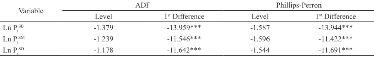
Table 1 represents the unit root test results. There are
Augmented Dickey-Fuller (ADF) and Phillips-Perron tests to confirm stationarity for each price. The test results show that the ADF test fails to reject the null
hypothesis of a unit root for each price in levels.
Meanwhile, the first differences of each price generate stationarity as the ADF test rejects the null hypothesis.
The Phillips-Perron test provides that the results fail to
reject the null hypothesis using level price and reject
the null hypothesis of stationarity for each price in
the first difference. The results signify soybean and its joint products significantly integrated of order one I(1), which is non-stationary. With the proof that the
price series is non-stationary, the test for cointegration
between soybean joint product prices pairs using
Table 1. Unit root test
Variable ADF Phillips-Perron
Level 1st Difference Level 1st Difference
Ln PtSB -1.379 -13.959*** -1.587 -13.944***
Ln PtSM -1.239 -11.546*** -1.596 -11.422***
Ln PtSO -1.178 -11.642*** -1.544 -11.691***
*** Significant at 1% level of probability; Source: Author’s Calculation, FAO (2019)
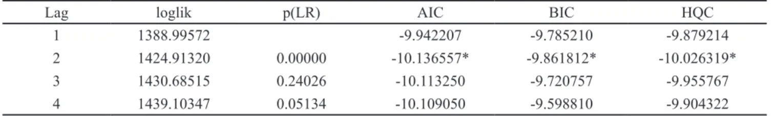
Lag Length Selection
Several test statistics like Akaike Information AIC, BIC, and HQ Criterion were used to select the order of the VAR model in Johansen’s cointegration technique
and VECM. To choose each model’s optimal lag length, the log-likelihood function model was maximized. That was done by selecting the model with the lowest criterion and cross-checking every single result to ensures accuracy.
All three criteria held two lags for the best choice
as a compromise between the goodness of fit and parsimonious of the model. In Table 2, the VAR lag
order selection results provided several options for length, which all the criteria suggested an optimal
lag of two. It would be appropriate and fit with the
model. The small number of lags retained a high degree of freedom and avoided increasing the likelihood of multicollinearity.
johansen Cointegration Test
The Johansen cointegration test was used to detect
if non-stationary prices of soybean joint products move together in the long-run. Since the price pattern
indicated that the series had constant without trend, restricted constant applied in cointegration and vector error correction model. By adding the restriction, it was assumed that there were no linear time trends
in the levels of the data. This specification enabled
the cointegrating equations to be stationary around a constant mean, but it did not allow for any other trends or constants.
The results of the cointegration analysis were
summarized in Table 3. To acquire a complete
perspective, the Johansen test was used to examine each
possible pair of soybean joint products, both in single
pair and simultaneous analysis. The Johansen test failed
to reject the null hypothesis of no cointegration between
soybean and soybean oil prices. Correspondingly, the
result denoted the pair price of soybean and soybean oil
was not cointegrated. However, there was evidence of a cointegrating relationship in Soybean and soybean meal price at a 10% significance level, but the simultaneously
model seems to give superior interpretation since it had
a higher significance level.
Furthermore, when the Johansen test included all three prices together as the dependent variable, there was at least one cointegration vector linking the
markets. The result rejected the null hypothesis of no cointegration but failed to reject the null hypothesis of
one cointegrating vector. Thus, this result reveals the existence of a long-run relationship between soybean, soybean meal, and soybean oil prices simultaneously.
Hence, it can be concluded that since all prices were
cointegrated, VECM was used to observe the extent of their elasticity relationship.
vector Error Correction Model
The Johansen test output gave a superficial overview
of the error correction mechanism. Cointegration test results demonstrated that there was one equilibrium relationship between the three prices in the long run. That implied the series was related and could be combined linearly.
From the results of the cointegration test, it was also
possible to check whether the signs of the coefficients
are in line with the prediction of economic theory.
According to Gardner’s joint-products equation (1987),
the price of soybeans can be represented as a weighted average of returns from soybean meal and soybean oil
less the processing (crushing) margin.
To resembles this theoretical expectation, the equation
must be normalized. The coefficient for soybean price
is the system’s endogenous variable and placed to the left-hand side while soybean meal and soybean oil are exogenous. Thus, the underlying long-run relationship is:
Table 2. VAR lag order selection criteria
Lag loglik p(LR) AIC BIC HQC
1 1388.99572 -9.942207 -9.785210 -9.879214
2 1424.91320 0.00000 -10.136557* -9.861812* -10.026319*
3 1430.68515 0.24026 -10.113250 -9.720757 -9.955767
4 1439.10347 0.05134 -10.109050 -9.598810 -9.904322
* indicates lag order selected by the criterion; Source: Author’s Calculation, FAO (2019)
Table 3. Johansen cointegration test
Dependent
Variable Rank Trace Test p-value L-max Test p-value Result
Ln PtSB 0 18.652 0.0814 15.735 0.0511 r=1* Ln PtSM 1 2.9168 0.6027 2.9168 0.6031 Ln PtSB 0 16.469 0.1558 13.849 0.1028 r=0 Ln PtSO 1 2.6205 0.6587 2.6205 0.6575 Ln PtSM 0 12.445 0.4183 9.9506 0.3504 r=0 Ln PtSO 1 2.4944 0.6822 2.4944 0.6810 Ln PtSB 0 56.524 0.0000 43.940 0.0000 r=1*** Ln PtSM 1 12.584 0.4064 10.090 0.3376 Ln PtSO 2 2.4946 0.6821 2.4946 0.6810
*** means significance difference P<0.01, ** 0.05, * 0.10; Source: Author’s Calculation, FAO (2019) Note: with restricted constant and two lags
As expected, the estimation of soybean price functions
has produced positive signs on its joint products, soybean meal, and soybean oil price . Since oil and
meal are both produced from the bean, the price of a bean is a weighted average of the oil and the meal prices, with weights roughly equal to the shares of oil and meal, respectively, in each quantity of beans. Based on the cointegration equation, assumed other things equal, each percentage-point increase in soybean
meal would cause an increase of 0.492 percentage points
in soybean price. Additionally, each percentage-point increase in soybean oil price has an effect of increasing
soybean price about 0.442 percentage points.
However, this positive coefficient probably gives
another perspective about the relation of soybean and
its joint products associated with their market. Recall that this research did analyze Rotterdam soybean price, Hamburg soybean meal price, and Dutch soybean oil
price. Now, associated with the cointegration equation,
positive constant reveals that soybean Rotterdam price
exceeds the weighted average of the Dutch oil and the
Hamburg meal prices. This result indicates soybean Rotterdam not processed by European domestic
processors to obtain Dutch Oil and Hamburg meals. Processing soybean Rotterdam will make losses for the processor. Hence, perhaps the soybean Rotterdam price has no joint product correlation towards Hamburg meal
and Dutch oil price.
This result in line with the previous study. Pritchett
et al. (2006) revealed that there is a weak correlation
between crush margin towards soybean, meal, and oil future price. Their analysis shows that estimated crush margins do not follow the same monthly average
price pattern as soybean and its joint products. This reflects the fact that considering the crush margin as
a linear dependence of soybean price is not too clear, particularly when the price associated with complex trade action. This evidence then reinforced by another
literature. Piggott and Wohlgenant (2002) indicated that the elasticities relationship of joint products and the
raw product are not straightforward if they are traded internationally, and there are policy interventions. Both literature results strengthen the assumption that
there is no crushing process from Rotterdam soybean to produce neither Hamburg meal nor Dutch oil. This is plausible because, mostly, the EU satisfies their
domestic soybean demand by importing them. The EU is the biggest soybean meal importer to meet the demand, mostly for their livestock feed. To produce
vegetable oil, they are centered on processing rapeseed
and sunflower seed. In other words, there are not many
domestic processors in the EU doing the soybean
crushing process (USSEC, 2008).
In short, considering the crush margin as the constant
of the joint products in the international price equation
perhaps generates misinterpretation, particularly when regressing the model with the international price.
However, it possibly fits the joint products model at the
domestic or farm price level, where there is minor price
intervention occurs. However, even though there is no joint product correlation between all three prices, they
remain to have a long-run relationship.
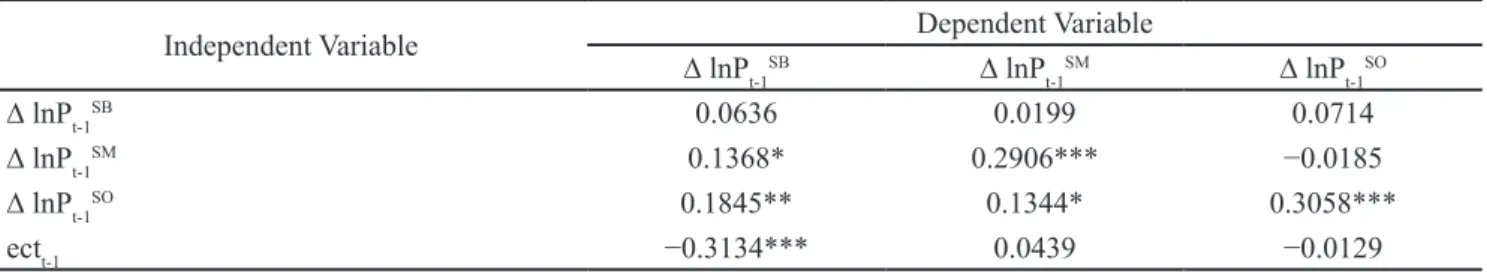
The estimation results for the short-run model included the ectt-1 from the long-run equation presented in Table
4. The corresponding adjustment coefficients for each equation were -0.3134 for the soybean, 0.0439 for soybean meal, and -0.0129 for soybean oil. However, the adjustment coefficient in the soybean meal and soybean oil price equation were not statistically significant. The adjustment towards the long-run equilibrium took place only through changes in soybean prices. Soybean price
is the only price that reacts to the correct equilibrium. This plausible because the markets for oil and meal are plentiful. The increases in meat consumption globally are expected to lead to increased livestock production, at the same time boosting the demand for soybean meal for feed use. Moreover, the broad demand for food, industrial applications, and biofuel makes soybean oil do not follow both meal and soybean prices.
Additionally, there are many substitutes that soybean meal and soybean oil must compete with. There are several substitutes for a protein source, namely corn, cottonseed, and rapeseed. Meanwhile, soybean oil must compete with palm and rapeseed oil, the closest substitutes to produce edible oil and biodiesel.
Therefore, the prices of both oil and meal are perhaps more exogenous, and the price of soybeans is always
adjusting as the weighted average of the prices of meal
and oil to changes in the prices of these two products.
The significant negative coefficient on ectt-1 indicated that soybean price responded to a temporary disequilibrium between three prices. The negative error
correction coefficient in the first equation of -0.3134
indicated that the soybean price got back to equilibrium
at 31% each month when there was a shock. Moreover,
when the average bean price was too high, it gradually fell back to correct the equilibrium.
This is not so fast as expected. One possible reason for
this relatively slow error correction could be because
there is no crushing process between soybean joint
products. The crushing process at a domestic level probably transmits the price transmission rapidly.
However, the exogenous variable, such as demand for
other oilseeds, dollar depreciation, restriction policies,
GMO issues, and crush spread speculation, perhaps more significantly affect the adjustment price but take a longer time. Hence, the adjustment process to restore
the equilibrium cannot be fast.
vECM Diagnostic Test
After estimation has been carried out, and the results have been obtained, several tests would be carried out to determine how adequate the model. First, the
Lagrange-multiplier (LM) test was performed to detect
the existence of autocorrelation in the residuals up to
the lag order of 12. At the 5% and 10% significance level, the null hypothesis could not be rejected either
with one or two lags. This revealed that the residuals of
the model did not seem to be affected by a significant
autocorrelation. Therefore, no evidence of model
misspecification was identified. Table 4. VECM estimation results and test
Independent Variable Dependent Variable
∆ lnPt-1SB ∆ lnPt-1SM ∆ lnPt-1SO
∆ lnPt-1SB 0.0636 0.0199 0.0714
∆ lnPt-1SM 0.1368* 0.2906*** −0.0185
∆ lnPt-1SO 0.1845** 0.1344* 0.3058***
ectt-1 −0.3134*** 0.0439 −0.0129
*** means significance difference P<0.01, ** 0.05, * 0.10; Source: Author’s Calculation, FAO (2019) Note: with restricted constant and two lags
permanently increase by about 0.027 % in bean price.
Both the positive response from soybean price gradually incline until the sixth period when it hits steady-state value and remains in the positive region.
Thirdly, it depicts the response of soybean towards its price shock. Interestingly, 1% of shocks in soybean price will cause a temporary increase to its rice from
0.052% to 0.058%. After hits a peak in the first period, there is a quick decline in the next period to 0.057%.
Further, the response value continues to decrease slowly until the tenth period and hits a steady-state value of
0.048%. This movement response indicates that if there
is a shock occurs in soybean price, it will correct its price to obtain equilibrium in the long-run.
When impulse response function is adopted to represents the shock effect of internal soybean
joint-products price, variance decomposition can be used to
evaluate the influence of each price change on other
prices that show relative impacts. According to bean price predicted variance, the contribution of bean price
change begins to decline from the first period quickly, reaches 80% in the fifth period, and then stably drops to 67% in the fifteenth period.
The oil price contribution rate gently rises to 16% in the tent period and then slightly increases to 18% until the last period. At the same time, the contribution
rate of meal prices slowly rises to 12% in the tenth
period and then basically maintains stability. In other words, soybean oil has more contribution to soybean price change compared to soybean meal. This possibly
reflects the facts already mentioned that soybean oil
more highly-priced than soybean meal. It can be seen
from the price movement provided by FAO, soybean
oil prices always higher than meal and bean prices for the last decades. This occurred due to the oil extracted from soybean is the main product for various uses and
the demand for it is also huge (USSEC 2008). Hence,
soybean price tends to follow soybean oil price compare to its meal and own prices.
Managerial Implications
This research identified whether there was a significant
long-term relationship among these three variables through cointegration tests and VECM. Impulse response and variance decomposition were also performed to interpret the results.
Besides, a test was performed to assess whether the
model satisfies eigenvalue stability and cointegration conditions. Stability test VECM was said to have
high stability when the characteristic polynomial of
autoregressive has modulus ≤1. The result showed that the modulus of the characteristics of roots at all lag is ≤1.
Thus, it can be concluded that the model is appropriate to be used since it has high stability. Moreover, the ADF
test for the cointegrating term rejects the null hypothesis of a unit root in level at a 1% significance level. This
showed that the cointegrating term obtained from the estimated VECM was stationary. The zero average lines represented a stable and long-term equilibrium relationship among variables, as predicted by theory. Nevertheless, the situation was worse regarding the vector tests for residuals normality via the Jarque-Bera test. Judging by the low p-values, the null hypothesis of
normality in every equation was rejected at conventional significance levels of 1%. This indicated that every
single equation contained non-normality residual and
probably lead to model misspecification.
However, violating the normality assumption might
not be a serious issue given the premise of asymptotic
normality insufficiency large sample size and with the condition that other assumptions hold (Wooldridge, 2002). Consequently, since all the previous test
indicated the reasonability of the model estimation, further steps of the analysis can undertake.
Impulse Response and variance Decomposition
Impulse response functions depict the effects of shocks
on the adjustment path of the bean prices towards meal and oil prices; meanwhile, forecast error variance
decompositions will measure the contribution of each type of shock to the forecast error variance. Both computations are assessing how shocks of meal and oil prices reverberate by soybean prices through a system. The horizontal axis represents the period in 15 months, while the vertical axis shows the response value in percent.
The IRF reveals that a one-time positive shock from
meal and oil price leads to a permanent increase in soybean price. Firstly, the result explains that a 1% increase in meal price will induce a continuous rise
in the bean price of 0.03%. Secondly, another IRF
Interestingly, based on the results of this study, changes
in soybean prices did not significantly affect the price of its oil and meal. However, the price change in soybean oil and meal only significantly affected by its
price in the last period. The price change for oil and
meal perhaps more influenced by other factors and
other markets.
Regarding the soybean market, the world's need for soybean and its joint products creates a competitive
market worldwide. For example, soybean products compete with wheat as human food, soybean meal competes with corn as feed, and soybean oil competes with palm oil like vegetable oil. Besides, the contribution of soybean and soybean meal as a source of protein is also dominant globally.
However, the contribution of soybean oil as a source of
vegetable oil was still inferior to palm oil, where palm
oil production was still dominated by Indonesia (OEC, 2020). This competition put palm oil and soybean oil in
the same market and perhaps affect one and another. Policy stakeholders in Indonesia should consider this
soybean joint products price transmission. As the largest producer of palm oil (USDA, 2019), the stakeholder
should maintain the price change in palm oil to compete
with the soybean oil price. Since soybean oil price is more independent from another joint product effect, it
perhaps has a stable price in the market and possibly creates a though competition for Indonesia’s palm oil market.
Simultaneously, Indonesia also the largest importer of soybean meal (OEC, 2020). Importing soybean meal
rather than import soybean and process it domestically is the recommended decision. This research implies that soybean meal price is more independent than soybean meal. This means that the price of soybean meal has greater stability than the soybean. It probably creates a good environment for the food and feed industry.
CONCLUSIONS AND RECOMMENDATIONS
Conclusions
There was one cointegration among soybean and its
joint products. Since oil and meal are both produced
from the bean, the price of a bean is a weighted average of the oil and the meal prices. Assumed other things
equal, each percentage-point increases in meal price
will cause a rise of 0.492 percentage points in bean
price. Additionally, each percentage-point increases in oil price have an effect of increasing bean price about
0.442 percentage points.
Although, the positive constant of the cointegration equation was violated the expected theory. This
constant reveals that soybean Rotterdam price exceeds the weighted average of the Dutch oil and the Hamburg meal prices. This indicates soybean Rotterdam price has no joint product correlation towards Hamburg meal
and Dutch oil price. This is in line with the previous study that presents there is a weak correlation between
the crushing margin and soybean joint products,
particularly in the global market.
VECM empirical results indicated that in the long-run, soybean price is the only one that reacts to correct equilibrium. This is reasonable since oil and meal have huge markets. Moreover, several possible
substitutes can easily switch the demand of these joint
products. If there is a shock, the soybean price gets
back to equilibrium at 31% each month. However, this adjustment speed is not so quickly as expected
since probably there is no actual relation between all
variables; perhaps other exogenous variables have more significant influence to make soybean correcting
the equilibrium slower.
An interesting conclusion was reached when the pattern of the impulse response functions was compared.
Soybean prices respond to meal and oil price shocks
with a steady increase of up to the sixth month.
However, when there is a shock in soybean price, its
price will decline slowly to correct the deviation, until it
hits constant value in the fifteenth month. According to
FEVD results, soybean oil generates more contribution to soybean price change compared to soybean meal. This perhaps occurs since soybean oil has the highest price among these products. Thus, soybean price change tends to follow its oil price rather than its meal and its prices.
Recommendations
However, some limitations should be noted. This
research regressed the variable of the international price
that possibly violated the soybean joint products theory.
A further research step may be to analyze the price at
Margarido MA, Turolla FA, Bueno CRF. 2007. The
world market for soybeans: price transmission into Brazil and effects from the timing of crop and trade. Nova Economia 17(2):241–270. OEC. 2020. Soybean Meal. The Observatory of
Economic Complexity, Massachusetts. https:// oec.world/en/profile/hs92/2304/. [29 Jan 2020]. . 2020. Soybean Oil. The Observatory of Economic
Complexity, Massachusetts. https://oec.world/ en/profile/hs92/1507/. [29 Jan 2020].
. 2020. Soybean. The Observatory of Economic Complexity, Massachusetts. https://oec.world/ en/profile/hs92/1201/. [29 Jan 2020].
Piggott NE, Wohlgenant MK. 2002. Price elasticities, joint products, and international trade. The
Australian Journal of Agricultural and Resource Economics 46(4):487–500.
Pritchett T, Smith A, Johnson T. 2016. Implications for Soybean and Livestock Producers From Relationships in The Soybean, Soybean Oil and Soybean Meal Markets. Department
of Agricultural and Resource Economics,
University of Tennessee, Institute of Agriculture, Tennessee.
Soon BM, Whistance J. 2019. Seasonal soybean price transmission between the U.S. and Brazil using
the seasonal regime-dependent Vector Error Correction Model. Sustainability 11(19): 1–9. USDA. 2019. Oilseed: World and Markets Trade.
The United States Department of Agriculture, Washington. http://apps.fas.usda.gov/psdonline/ psdDataPublications.aspx [29 Oct2019].
USSEC. 2008. How the Global Oilseed and Grain Trade Works. The United States Soybean Export Council, Missouri. https://ussec.org/wp-content/ uploads/2015/10/How-the-Global-Oilseed-and-Grain-Trade-Works.pdf. [29 Jan 2020].
Wohlgenant MK. 1999. Product heterogeneity and
the relationship between retail and farm prices. European Review of Agricultural Economics
26(2):219–227.
Wooldridge JM. 2002. Introductory Econometrics: A Modern Approach. Mason: South-Western
College Publishing.
Zaytsev O. 2010. The impact of oil price changes on
the macroeconomic performance of Ukraine
[Thesis]. Ukraine: Kyiv School of Economics.
model. Furthermore, it is essential to consider involving
exogenous variables that perhaps significantly affect the price transmission of soybean and its joint products. Lastly, this study can help traders and policymakers
understand that there is a price transmission occurs
in soybeans and its joint products’ prices, globally.
For instance, the changes in soybean oil prices of the biodiesel market perhaps affect the meal and bean prices for animal feed and human food markets. This dynamic of the soybean market must be considered to maintain the stability of prices and supplies of each soybean products.
REFERENCES
Arnold BC, Balakrishnan N, Alegria JMS, Minguez R. 2008. Advances in Mathematical and Statistical Modeling. New York: Springer Science, and
Business Media.
Brooks J, Melyukhina O. 2003. Estimating the
pass-through of agricultural policy reforms: an
application to Russian crop markets, with possible extensions, mimeo, OECD, Paris. Brooks C. 2008. Introductory Econometrics for
Finance. Cambridge: Cambridge University Press.
Enders W. 2015. Applied Econometrics Time Series.
New Jersey: John Wiley and Sons.
Engle RF, Granger CWJ. 1987. Cointegration and
error correction: representation, estimation, and testing. Econometrica 55(2):251–276.
FAO. 2019. GIEWS FPMA Tool. Food and Agriculture Organization of the United Nations, Rome. http:// www.fao.org/giews/food-prices/tool/public/#/ dataset/international. [29 Oct 2019].
Freitas SM, Margarido MA, Barbosa MZ, Franca TJF. 2001. Análise da dinâmica de transmissão de
preços no mercado internacional de farelo de
soja. Agricultura em São Paulo 48(1):1–20. Gardner B. 1987. The Economics of Agricultural
Policy. Washington D.C.: Macmillan Publishing
Company.
Hamilton JD. 1994. Time Series Analysis. New Jersey: Princeton University Press.
Hill RC, Griffiths WE, Lim GC. 2011. Principles of Econometrics. New Jersey: John Wiley and Sons.