Price variability and the speed of adjustment to the law of one price: Evidence from Slovakia

Julius Horvath and Stanislav Vidovic

Price variability and the speed of

adjustment to the law of one price:

Evidence from Slovakia

B a n k o f F i n l a n d

BOFIT – I n s t i t u t e f o r E c o n o m i e s i n T r a n s i t i o n

Mr Timo Harell, editor Press monitoring

Editor-in-Chief of BOFIT Weekly Timo.Harell@bof.fi

Ms Liisa Mannila, department secretary Department coordinator

Publications traffic Liisa.Mannila@bof.fi

Ms Päivi Määttä, information specialist Institute’s library

Information services Paivi.Maatta@bof.fi

Ms Tiina Saajasto, information specialist Statistical analysis

Statistical data bases Internet sites

Tiina.Saajasto@bof.fi

Ms Liisa Sipola, information specialist Information retrieval

Institute’s library and publications Liisa.Sipola@bof.fi

Information Services

Mr Pekka Sutela, head

Russian economy and economic policy Russia’s international economic relations China in the world economy

Pekka.Sutela@bof.fi

Bank of Finland

BOFIT – Institute for Economies inTransition PO Box 160 FIN-00101 Helsinki

Contact us

Chinese economy and economic policy Gang.Ji@bof.fi

Ms Tuuli Koivu, economist

Chinese economy and economic policy Editor-in-Chief of BOFIT China Review Tuuli.Koivu@bof.fi

Mr Tuomas Komulainen, economist Russian financial system

Currency crises

Editor-in-Chief of BOFIT Online Mr Iikka Korhonen, economist

Exchange rate policies in transition economies Monetary policy in transition economies Iikka.Korhonen@bof.fi

Mr Vesa Korhonen, economist Russia’s international economic relations

Russia’s banking system

Vesa.Korhonen@bof.fi

Ms Seija Lainela, economist Russian economy and economic policy Editor-in-Chief of BOFIT Russia Review Seija.Lainela@bof.fi

Mr Jukka Pirttilä, research supervisor Public economics

Transition economics

Editor-in-Chief of BOFIT Discussion Papers Jukka.Pirttila@bof.fi

Mr Jouko Rautava, economist Russian economy and economic policy Jouko.Rautava@bof.fi

Ms Laura Solanko, economist Russian regional issues

Public economics Laura.Solanko@bof.fi

Ms Merja Tekoniemi, economist Russian economy and economic policy Merja.Tekoniemi@bof.fi

Price variability and the speed of

adjustment to the law of one price:

Evidence from Slovakia

BOFIT Discussion Papers 3/2004 26.2.2004

Julius Horvath and Stanislav Vidovic:

Price variability and the speed of adjustment to the law of one price: Evidence from Slovakia

ISBN 951-686-888-6 (print) ISSN 1456-4564 (print) ISBN 051-686-889-4 (online) ISSN 1456-5889 (online)

Suomen Pankin monistuskeskus Helsinki 2004

3

Contents

3.1 The static absolute law of one price ...12

4 Relative price variability in districts and individual price variability across districts...14

5 The speed of adjustment ...20

6 Conclusions ...22

References ...23

Tables ...25

4

All opinions expressed are those of the authors and do not necessarily reflect the views of the Bank of Finland.

5

Julius Horvath

and Stanislav Vidovic

Price variability and the speed of adjustment to the law

of one price: Evidence from Slovakia

Abstract

This paper uses a large panel data set of monthly frequency final good and service prices in thirty-eight Slovak districts over a five-year period to study price variability and the work-ing of the law of one price. We concentrate on three issues. First, uswork-ing simple statistical tools, we investigate the range of price differences across Slovak districts. Second, we measure relative price variability across cities and across products. The variability of rela-tive prices in the same district appears to be higher than the variability of prices of the same good across different districts. We identify the factors likely to be responsible for this fact. Third, using benchmarks we investigate the speed of convergence to the absolute law of one price. While we find evidence for absolute convergence, the speed is lower than that found in US cities. The speed of convergence to the relative law of one price is considera-bly higher.

† _{Corresponding author. Department of International Relations and European Studies, Central European} Uni-versity, Budapest and Faculty of Social and Economic Sciences, Comenius UniUni-versity, Bratislava. e-mail: horvathj@ceu.hu

‡ _{Department of Economics, University of Rochester. E-mail: svidovic@troi.cc.rochester.edu}

∗ _{We thank Attila Ratfai, and Iikka Korhonen for helpful comments and useful suggestions on the earlier} draft of this paper. Also we thank participants in the workshop at the Bank of Finland, BOFIT and at the Technical University in Vienna for their suggestions and comments. We also thank Ronald Blasko for pro-viding us with the data. All remaining errors are of course ours.

6

Julius Horvath and Stanislav Vidovic

Price variability and the speed of adjustment to the law

of one price: Evidence from Slovakia

Tiivistelmä

Tässä työssä tutkitaan yhden hinnan lain toteutumista ja hintojen vaihtelua laajan hinta-aineiston avulla. Käytössä on kuukausittaisia havaintoja yksittäisten tavaroiden ja palvelui-den hinnoista Slovakian 38 hallintoalueesta viipalvelui-den vuopalvelui-den ajalta.Ensiksi selvitetään yksin-kertaisilla tilastollisilla menetelmillä hintojen vaihtelua Slovakia hallintoalueiden välillä. Seuraavaksi mitataan suhteellista hintavaihtelua tuotteiden ja kaupunkien välillä. Suhteel-listen hintojen vaihtelu hallintoalueiden sisällä näyttää olevan suurempi kuin yksittäisten tuotteiden hintojen vaihtelu hallintoalueiden välillä. Tutkimuksessa selvitetään tekijöitä, jotka aiheuttavat tämän. Kolmanneksi, lasketaan kuinka nopeasti hinnat konvergoituvat absoluuttisen yhden hinnan lain määrittämään hintatasoon. Tuloksien mukaan hintakon-vergenssia on, mutta sen nopeus on vähäisempi kuin yhdysvaltalaisten kaupunkien välillä. Hintakonvergenssi suhteellisen yhden hinnan lain määrittämään hintatasoon on selvästi nopeampaa.

7

1

Introduction

The study of the law of one price (LOOP)1 and its aggregate version, the purchasing power parity (PPP) has a long history in international economics.2 However, till now, only a small number of papers3 attempted to tackle the LOOP in the context of transition economies. This paper examines the concept of the law of one price using store level price data in the context of a small open transition economy, Slovakia.

The paper begins with a direct, unconditional description of the behavior of consumer price data across regions in Slovakia and finds that they seem to be for the most part incon-sistent with the simple static absolute version of the LOOP. Simply, in a given time period the differences between nominal prices seem to be too large for the LOOP to hold. In a given period of time the differences between non-homogeneous products were in some cases in hundreds of a percent. The differences are lower for homogeneous products, but 30-50 percent differences even for these products are quite common. However, most prices move together across districts and within a band.

Then, we analyze the variability of relative prices across districts and across products. Here we follow the empirical strategy proposed in Engel and Rogers (2001). Our results support the following empirical regularity: the variability of relative prices within the same district is higher than the variability of prices of the same good across different districts. The variability of the price of consumer good i relative to good j in the same district is higher than the variability of consumer good j across different districts. In other words, the price of beef relative to the price of chicken in a given district is more variable than the price of beef across all districts.

1 _{The cornestore of the LOOP is consumer arbitrage across different locations. In the long run, adjusted for}

transportation costs, prices of goods and services measured in the same currency should be identical across all geographic locations. However, there are problems with the understanding of the LOOP even as an em-pirical proposition. Herrmann-Pillath (2001, p.48) writes: “adherence to the LOOP does not seem to be an empirical issue but a matter of basic beliefs about how the market mechanism works.” One can be of the opinion that under market imperfections, imperfect information, prevailing disequilibria, missing contracts and high search costs there may be good reasons for the LOOP not to hold. On the other hand, there is always the argument that these frictions may disappear in the long run.

2 _{The most recent discussions include, among others Engel (1993), Parsley and Wei (1996), Engel and} Rogers (1996), Cecchetti, Mark and Sonora (1999), Engel and Rogers (2001), Haskel and Wolf (2001), Imbs, Mumtaz, Ravn and Rey (2002), and O’Connel and Wei (2002).

3 _{See Conway (1999), Cushman, MacDonald and Samborsky (2001), Wei and Fan (2002), Ratfai (2003) and} Vidovic (2003).

8

Finally, we also investigate relative price reversion to a common mean employing the panel unit root test of Levin and Lin (1992). In the international context it is often demon-strated that mean reversion in relative prices does occur but that it is slow, taking between three and five years. We ask whether these results also hold for regions inside the currency area. In general, one may expect faster price convergence across regions than across coun-tries, as is documented for developed market economies.4 _{For Slovakian regions, this is} less obvious. On one hand, there are good reasons to expect Slovak regions to be integrated with each other. These regions have the same heritage and language (some exceptions may be found in the southern regions but even there Slovak is widely used), and had largely free capital, labor and product markets during the period under investigation. Also these regions share the same currency and the distance between them is insignificant. On the other hand, there is a tendency in Slovakia toward pronounced economic disparities across regions.5 The empirical results show that there is evidence of convergence to the LOOP in Slovak data. However, our results indicate that the speed - while faster than typically found in cross-country data - is lower than that found in US cities.

This paper is structured as follows. In Section 2, we describe the price data. In section 3, we take a first glimpse at the data. In Section 4, we measure the variability of relative prices across products and districts. In Section 5, we measure the speed at which prices converge, and in the last Section, we summarize and conclude.

2

The data

Our data set contains monthly frequency nominal prices for more than five hundred final goods and services from 38 Slovak districts over the period from January 1997 to Decem-ber 2001.6 The data are thus three dimensional, the dimensions being time, commodity,

4 _{However, Cecchetti, Mark and Sonora (1999) find that deviations from city purchasing power parity are} more persistent than deviations from international PPP.

5 _{This is well documented in Kárász, Kárász and Pala (2000) and World Bank (2002).}

6 At this time the Slovak economy had moved away from the monetary overhang that was inherited from the past and possibly impacting on relative prices. Also, as some prices - especially in transportation and utilities - were tightly regulated and the Central Bank of Slovakia pursued a relatively tight monetary policy in this period, the inflation rate was low as compared to the early 1990s.

9

and district.7 Store identifiers are not available in the sample. The full data set includes tradable and nontradable goods and services, homogeneous and heterogeneous products.8 Depending on the aim of the particular investigation, we also select sub-samples from the data. For purposes of the empirical analysis, we calculate district specific cross-store aver-ages from the individual prices.

These data serve as the basis for calculation of the consumer price index by the Slovak Statistics Office (SSO), which provides explicit instructions and data forms to data collec-tors. The collector typically obtains the data by visiting the premises (shops) by the 20th of the respective month. Then data are sent to a particular branch of the Statistics Office. The explicit instructions of the SSO allow consideration of domestic as well as imported goods and goods of different quality, but not goods of lower than the ‘first quality category.’ The consumer prices of final goods and services are provided inclusive of value-added tax. Col-lectors of price data may use sale prices of products that are accessible to all consumers. SSO encourages this, especially if these sales are temporary and it is expected that the products will be sold again at ‘normal’ price. Importantly, the data set contains actual prices rather than quoted prices or price indices. The stores are selected by the SSO repre-sentative and may include privately and publicly owned stores. In case a store is not oper-ating any more, it is replaced by a comparable store in the same district, but only upon prior approval of the SSO branch office. It is important to note that SSO collects prices from at least three different stores in each district. For food and catering in the services sectors, cheaper, middle level, and high price stores are considered. In apartment rent prices, at least two prices are provided: one from the downtown (city center) and the other from the outskirts.

The products in the sample represent basic foodstuff, alcoholic beverages and tobacco, as well as clothing, footwear, housing, water, electricity, gas and other fuels as well as fur-nishings, household equipment and home maintenance. Finally, the data set also contains

7 We use the regional division in Slovakia with 38 districts. The data collected in the sample are almost ex-clusively taken from the capital cities of the districts. The districts are the following: Bratislava, Bratislava-vicinity, Dunajská Streda, Galanta, Senica, Trnava, Považská Bystrica, Prievidza, Trenčín, Komárno, Levice, Nitra, Nové Zámky, Topolčany, Čadca, Dolný Kubín, Liptovský Mikuláš, Martin, Žilina, Banská Bystrica, Lučenec, Rimavská Sobota, Veľký Krtíš, Zvolen, Žiar nad Hronom, Bardejov, Humenné, Poprad, Prešov, Stará Ľubovňa, Svidník, Vranov nad Topľou, Košice, Košice-vicinity, Michalovce, Rožňava, Spišská Nová Ves, Trebišov.

8 By homogeneous product we mean an item that consumers may consider as perfectly (or almost perfectly) substitutable across different suppliers.

10

prices on health; transport; restaurants and hotels catering and accommodation services; personal care; recreation; and culture. Consequently the data set contains low priced items (matches, salt) as well as expensive items (durables). It also contains some nationally rec-ognized Slovak brand names.

3

A first glimpse

In this Section we carry out a preliminary analysis of the degree of deviation from the LOOP. Our data set allows us to abstract from the effects of nominal exchange rates, trade policies, and similar issues arising in an international context. With disaggregated data on actual consumer prices for different types of products, we also avoid aggregation problems associated with using sector level price indices. On the other hand we are aware of the fact that by not using general price indexes, but instead using nominal absolute average prices of selected individual goods, our data set may seem to be too specific. In this respect Has-kel and Wolf (2001) note the following: “abandoning price indices for actual transaction prices comes at a cost: by necessity, any group of products selected has some ‘special’ characteristics that may limit the extent to which finding for that group can be general-ized.” At the same time, if any version of the law of one price is to hold, it should hold on the individual level if it is to hold at all.

We begin with some simple data checks. First, Slovakia consists of eight basic regions. The World Bank (2002) compares regional GDP per capita at purchasing power and finds that in 1999 the Bratislava region was approximately 100% of the EU average, and all other regions were at 50% or below. Of the remaining seven regions, the Prešov region was the poorest, at 32% of the EU average. In light of this difference, one might expect that Bratislava-region prices would be higher than prices in the Prešov-region, especially for key products in daily consumption. Figure 1 gives boneless chunk roast prices for Bra-tislava and Svidnik (a district in the Prešov region). Despite the significant income gap, price levels in the two locations seem to move together quite closely. Prices in Svidnik are in some periods even higher than prices for the same product in the Bratislava district. One can find other food products displaying the similar patterns. For instance, Figure 2 showing the price behavior of wooden coffins, a more heterogeneous product, makes the picture

11

even bleaker; it is more expensive to get a coffin in Svidnik than in Bratislava. Though these observations are arguably a bit naïve, there are still lessons to be learned here. First, massive income differences across regions may not imply higher prices of particular prod-ucts in richer regions, even if one expects higher price levels in the more advanced regions. In richer districts one finds increased competition, which may push retail prices down as compared to poorer districts where small shops are still prevalent.

Second, the search costs may be particularly high if the product is inexpensive and not bought repeatedly, so that consumers may stop searching for the lowest price before buy-ing. Thus the factors that would support LOOP may be less effective with homogeneous and relatively inexpensive products. This seems to be confirmed for example by Figure 3, which describes the behavior of the retail price of matches in the 38 districts. The price dif-ferences between regions are huge and hence it seems that arbitrage is not prevalent. The emerging picture is quite different for gasoline prices, for instance, shown on Figure 4.9 The search cost for gasoline is presumably small, as it accounts for a substantial chunk of the consumer's budget, and is bought repeatedly.Third, search costs may be high for het-erogeneous products because of the time it takes to compare the different alternatives on the market. During the period studied, catalogue sales and computer shopping were not standard. Thus for heterogeneous products such as men’s leather sport-type footwear (or ladies stockings) one would expect that the factors supporting the LOOP would be weak. Evidence in support of this statement is provided in Figure 5.

Fourth, international chains of retail stores are moving gradually into the Slovakian market. Intuitively, one may expect convergence in price levels for products sold by these chains, especially for brand-name products. We do not have such products in our data set. However, our data set contains some products, which are brand names across Slovakia. These are Alpa Francovka (cosmetic alcohol used in Slovak households, inexpensive and not bought repeatedly), Cigarette Mars (widely consumed, especially by lower income in-dividuals), Cigarette Dalila (widely consumed, especially by middle income individuals) and Cheese Niva (a popular cheese brand name). Figures 6 and 7 plot the time paths of some of these national brand name prices in Slovak districts. As with many other prices, eyeballing these graphs suggests that some product prices move within a band. The widths of the bands however differ across products. In some cases the width is very narrow and

12

not increasing, in other cases it is large and seems to widen. This issue is taken up in a more detail in Section 5.

3.1

The static absolute law of one price

To take a snapshot of product prices at different locations at a given point in time, we in-troduce the notion of the static absolute law of one price (SALOOP). Let A

i

p and B i

p repre-sent the given-period price of the ith commodity in districts A and B, respectively. If SA-LOOP holds, these two prices are equal. Using simple descriptive statistics, we evaluate the validity of SALOOP. 10 As transport costs, price stickiness in local currency prices, non-competitive markets and other obstacles to arbitrage do exist even in national markets, our prior is that SALOOP will not hold. But even if there are differences between the prices, we still would like to know how large these differences are in the data.

To assess the extent of these differences we initially chose a set of 44 goods and di-vided them into food products (including tobacco) and non-food products. Most of the food and tobacco products represent homogeneous and tradable goods. They include rice, sugar, potato, milk, butter, eggs, oranges, poppy-seed, cheese ‘Niva’, wheat flour, white rolls, white bread, corn flakes, beef, pork, chicken, salami, coffee, candies, cigarettes and lettuce. Our second set of products involves some homogeneous non-food products such as Alpa Francovka, matches, children game Človeče Nehnevaj sa, cement, synthetic blanket Larisa, storage can Omnia, drivers license fee, and video-tape rentals. For illustration purposes, we also include products in this group, for which homogeneity is unlikely to hold. This latter group includes linen bed-sheet, ladies stockings, men's sport leather shoes, wooden coffin, men's boxer shorts, wedding dress rentals, meal in restaurant, apartment rent for 2 and 3 bedrooms, apartment painting, and ticket for classical theater performance.

The descriptive statistics for the forty-four products are presented in Table 1. Two rela-tive prices are given, as measured in April 2001: the difference between maximum and 9 _{Figures 3 and 4 each contain more than 2000 observation (60 times 38). To ease visualization, the graphs do} not contain a legend.

10 _{It may be that the concept of SALOOP holds only as equilibrium and thus when characterizing conditions} for it to hold one should refer to all basic laws of equilibrium analysis as consumer utility maximization and optimization. This fact is obscured in the empirical analysis, which considers only the movement of prices. Herrmann-Pillath (2001, p. 48).

13

minimum price observations (max-min) and the difference between maximum and mean price observations (max-mean) among the thirty-eight districts. The deviations in max-min relative price are on the order of 10 to 100 per cent. This max-min relative price is lowest for tobacco products and highest for white bread, white rolls, and rice.11 _{The max-mean} relative price ratio is understandably less variable; it fluctuates between 4 and 70 percent. The results presented in Table 1 do not change significantly if we look at the max-min and mean relative prices over time. For example Figure 8 plots the corresponding max-mean price ratio for boneless chunk roast.

Differences among non-food products are more pronounced. This must be partly due to the fact that heterogeneous goods are included in the sample. Large differences in max-min and max-mean relative prices obtain for lady’s apparel, men's shoes, and wooden coffins. On the other hand, the market for gasoline – homogeneous product in a highly competitive oligopolistic market - is extremely integrated, the difference between maximum and mini-mum average price across districts being only around 3 per cent, and the max-mean rela-tive price ratio around one per cent.

Observing these differences also begs the question: what accounts for them? Our prior is that distance would not play a major role in explaining these differences.12 One might also consider location-specific and goods-specific factors. If location-specific factors pre-vail, and if they are the sole reason for price differences across districts, then we may find similar patterns in the behavior of relative price pairs in each district and each product in the sample. To evaluate this conjecture we calculate pairwise relative prices for each dis-trict and each product in April 2001. For example, for the Bratislava disdis-trict we calculate the relative price as compared to other districts for each product, thus obtaining 2580 pair-wise relative price observations. Of these almost 75 percent were higher than one (price in Bratislava higher than that in the other district) as reported in Table 2. This ratio was high-est in Bratislava followed by Kosice. While the correlation between this measure of

11 _{Note that these differences are lower than differences reported by Haskel and Wold (2001) for identical} IKEA products across different countries. For some specific products in their sample they report the max-min relative price ratio to be higher than nine.

12 _{Evidence in Engel and Rogers (1996) suggests that distance explains much of the price variability of} simi-lar goods in the United States and Canada. We do not expect distance to contribute significantly to the expla-nation of the price variability in Slovakia. Slovakia is a small country - less than 50 thousand square kilome-ters. The furthest distance between most eastern and western parts of the country is less than 700 km, be-tween most northern and southern parts considerably less. The average distance bebe-tween pairs of capitals of the 38 Slovakian districts used in this study is around 190 km. Thus, while expecting distance to play some role in explaining the behavior of prices across districts it is our prior that this role will be rather limited.

14

wise relative prices and distance from benchmark city (Bratislava, Banska Bystrica) is in-significant, there is high positive correlation between pairwise relative prices and size of district, the latter measured as population of the district's capital. This indicates that there is a tendency for prices to be the higher, the larger the city, suggesting the existence of loca-tion (city) specific effects in pricing patterns across districts.13

4

Relative price variability in districts and

individual price variability across districts

Engel (1993) - studying sources of real exchange rate volatility across six developed coun-tries14 - uncovers an interesting empirical regularity: “the consumer price of a good relative to a another good within a country tends to be much less variable than the price of that good relative to a similar good in another country.” Engel (1993, p. 35). In other words, comparing the volatility of prices of the same (similar) goods across borders to volatility of different goods inside the same country, Engel (1993) presents empirical evidence that the volatility of the former is higher than the volatility of the latter. Engel and Rogers (2001) performed a similar investigation within the United States, and the results show that there is a tendency for prices of the same product across different cities to be less volatile than the prices of different products in a city. In other words relative prices of different goods in a city are more volatile than price of the same good across cities. The analysis in this section is inspired by the approach developed in Engel and Rogers (2001). However, our data comprise actual (average) monthly prices for 501 final goods and services over a five year period, whereas Engel and Rogers used monthly price indexes for 43 different goods and services over some ten years. Thus, we investigate two sources of variability in prices. First, we look at the variability of each individual price across districts; second, in each in-dividual district we look at the variability of prices of all products. Before we present the empirical analysis we provide some justification for this approach.

13 _{This may also reflect the price levels in these districts. Note that according to our knowledge there are no} data on regional price levels in Slovakia.

15

Consider two goods i and j, and two locations A and B and the following simple exam-ple of the real exchange rate between the two locations. Let capital letters denote price in-dexes and small letters prices of specific goods. Then

(1 ) A A A i j P =αp + −α p (1 ) B B B i j P =γp + −γ p

and their difference is

(1 ) (1 )

A B A A B B

i j i j

P −P =αp + −α p −γp − −γ p (1) These can be rewritten as

( ) (1 )( ) ( )( ) A B A B A B B B i i j j i j P −P =α p −p + −α p −p + α γ− p −p (2a) ( ) (1 )( ) ( )( ) A B A B A B A A i i j j i j P −P =γ p − p + −γ p − p + α γ− p −p (2b)

Equations (2a) and (2b) contain two types of expressions. The first compares the price of the same good (i or j) in two different locations (A and B). These are the first two expres-sions on the right hand side of equations (2a) and (2b). The second compares the prices of different goods (i and j) in the same location (A or B).

Comparing A, A, B, B

i j i j

p p p p in the static environment we may assume the following.

- Assuming that the law of one price holds, or there is a tendency for it to hold, then prices of similar goods converge across different districts, i.e. there is a tendency for

A B

i i

p = p and A B

j j

p = p . Then, if V represents volatility, one can expect V(piA - piB) to be

low and thus ( A A) ( A B)

i j i i

V p −p >V p − p . In other words, volatility of relative prices in the same district is higher than the volatility of prices of the same good across districts. However, this result may be obtained also if one assumes the same (similar) degree of price stickiness of an individual good across districts; then again ( A A)

i j

V p −p > ( A B)

i i

V p −p .

- Assuming that the law of one price does not hold for some reason (markets are seg-mented, producers have different pricing strategies for different locations, etc.), then one can expect that the same product would be priced differently in two locations, i.e.

A B

i i

p ≠ p and A B

j j

p ≠ p , and consequently one expects ( A A) ( A B)

i j i i

V p −p <V p − p . The same expectations hold if the distance between locations A and B is significant, and transportation costs or other trade barriers prevent the convergence of prices. Then again one can expect ( A A) ( A B)

i j i i

16 Thus ( A A)

i j

V p −p is a measure of volatility of relative prices in the same location and ( A B)

i i

V p −p a measure of volatility of the price of the same good in different locations. Fol-lowing Engel and Rogers (2001) we define ratio k

i r as , , 1, , , 1, 1 ( ) 1 1 ( ) l k k i t n t n n i k i h k m i t i t m m k sd p p l r sd p p h = ≠ = ≠ ∆ − ∆ − = ∆ − ∆

∑

∑

where sd(.) denotes standard deviation, l the number of products in the data set, and h the number of districts. k_,

i t

p is the log of the price of good i, at time t, at location k. Also, , , , 1 ln k i t k i t k i t p p p ₋ ∆ = , , , , 1 , , , 1 , 1 , , 1 / ln ln ln( ) / k m k k i t i t i t i t k m i t i t k m m m i t i t i t i t p p p p p p p p p p − − − − ∆ − ∆ = − = . The k i

r coefficient is the ratio of sums of standard deviations.

The numerator in (3) represents the average of the standard deviations of the first log difference of the price of good i relative to the price of each other good at location k. Thus, the numerator represents the volatility of relative prices of different goods in the same lo-cation.

The denominator in (3) represents the average of the standard deviations of the first log difference of good i at different locations, k and m. Thus, it is the denominator in (3) which measures the deviation from the LOOP. More precisely we may call it the measure of the relative law of one price, since here we really consider variation of log differences of two prices. If the relative LOOP holds, then the denominator is expected to be small. Engel and Rogers (2001) mention that there are actually three cases where one can expect the de-nominator to be small. First, when the ‘law of one price holds’, so that the differences be-tween the prices of good j in two locations are small. Second, if the price of good j at loca-tion A is proporloca-tional to the price of good j at localoca-tion B, the difference is almost constant. Third is the case where the price of good j at both locations is hardly changing.

We now turn to the analysis of the variability of prices in our data set. In reporting the results we divide the data set according to the following classification: Table 1 Bread, Ce-reals, Meat and Fish; Table 2 Milk, Cheese, Eggs, Oils and Fats; Table 3 Fruit, Vegetables

17

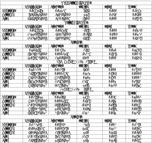
and Other Food Products; Table 4 Non-Alcoholic and Alcoholic Beverages and Tobacco; Table 5 Clothing; Table 6 Footwear; Table 7 Housing, Water, Electricity, Gas and Other Fuels; Table 8 Furnishings, Household Equipment and Routine Maintenance of the House; Table 9 Health; Table 10 Transport; Table 11 Recreation and Culture, Major Durables for Recreation and Culture; Table 12 Restaurants and Hotels Catering and Accommodation Services; Table 13 Personal Care. A general picture of the data set is provided in Table 3.

These results for coefficient k i

r are summarized in Table 4.15 The data show that the

k i

r coefficient is above one for all thirteen groups of products. In the sample of 501 indi-vidual products the k

i

r coefficient is greater than one in about 92 per cent of the cases. In the remaining cases – where it was smaller than one - the smallest value was 0.74.16 When we weight the coefficients (with weights equal to the weights assigned for each particular good in the consumer price index in 2002), the k

i

r coefficient is still, in more than 92% of the cases, higher than one. The results in Table 4 also show that the unweighted average of all k

i

r ratios equals 1.47. Taking a weighed average across products, the average k i

r in-creases to 1.86.17

There seem to be certain regularities in these results. The variability of relative prices in the same district is higher than the variability of the price of the same good across dif-ferent districts. In other words the price of a consumer good relative to a difdif-ferent good in the same district is more variable than the price of the same good across districts. This ob-servation suggest that the variability in real exchange rate is affected more by movements in the last factor on the right hand side of equations 2a and 2b than in the first two factors.

Columns 2 and 3 of Table 4 give the results calculated for monthly differences in the logs of prices. Columns 5 and 6 of Table 4 give the corresponding statistics for twelve-month differences. One may expect convergence to the relative LOOP to hold more as time passes, and a corresponding increase in the value of the k

i

r coefficient. The data show

15 _{Detailed results are available from the authors upon request.}

16 _{Engel (1993) found that for most of the goods the intra-country relative price changes are much smaller} than the failures of the inter-country LOOP. If these results were valid for the case of intra-country data, then the reported coefficients r_ikwould be small. Engel and Rogers (2001) wrote that average values would need to be around 0.15 to replicate the Engel (1993) finding. Results of Engel and Rogers (2001) as well as our results challenge this expectation.

17 _{In the sample used by Engel and Rogers (2001), the weighted average value of the coefficient was greater} than two.

18 a slight increase in the un-weighted value of the k

i

r coefficient, from 1.47 to 1.59, and a more significant increase in the weighted-value, from 1.86 to 2.59. This result to a certain extent differs from Engel and Rogers (2001) who reported that the twenty-four-month ra-tios “actually are slightly lower, which is the opposite of what one would expect.” (p.6).

As the next step we analyze the denominator of the k i

r coefficient.18 _{These results are} summarized in Table 5. Again, the denominator measures the average standard deviation of the difference in the price of the same good across cities, what we call the relative law of one price. In Engel and Rogers (2001), the weighted average of the denominator of the

k i

r coefficient equals 2.87; in our sample it is 4.47. This suggests that either the ‘absolute law of one price’ holds to a lesser extent in our sample than in theirs, i.e. prices are less proportional across districts in Slovakia than they are across the US cities, or the prices of the same good across Slovak districts are less sticky. An additional reason may be that our data contain individual actual prices whereas Engel and Rogers used price indexes, and the individual prices can be more volatile.19

The lowest denominator values in the calculations of Engel and Rogers (2001) are for ‘food away from home’ and ‘used cars’, where the relative variabilities are less than one. In our sample the lowest variability is for Aspirin (1.04), gasoline 91-octane (0.94), gaso-line 95-octane (1.09), and oil fuel (0.97). We find the highest volatility for tomato (41.95), parsley (32.37), kiwi (22.81), ignition module (17.82), apples (15.22), mandarins (13.94), fruit-based soft drink (13.69). This measure of variability is very high for fruit and vegeta-bles in both countries. But high volatility was also found among such non-tradavegeta-bles as ser-vices provided with apartment renting (13.31).

18 _{Engel and Rogers (2001) argued that the numerator is similar to the numerator analyzed in Engel (1993),} so that the larger r_ik ratios in Engel and Rogers (2001), as compared to Engel (1993) stem from the smaller value of denominator. Subsequently they concentrate on explanation of the value of the denominator. We follow their strategy with the following caveat. In Engel and Rogers (2001) the numerator measures the volatility of relative prices in 29 large U.S. cities. One needs to make an assumption that the competitiveness of local markets in these cities for different products is similar. This assumption excludes the following situa-tion: there is no tendency for the law of one price to hold, but the variation which this causes is smaller then the variation caused by the differences in market structures in different cities (regions). Thus, even if the law of one price does not hold, we may still obtain an r_ik coefficient greater than one. We also assume away this possibility for the Slovak regions.

19 _{It seems that this last reason is not born out by the data. There are disaggregated product prices in our} sam-ple with significantly higher volatility than the price indexes in Engel and Rogers (2003), but our data set also contains prices considerably less volatile than their more aggregated data.

19

Engel and Rogers (2001) also compare the value of the denominator of non-traded to traded goods; they simply classify goods as traded and services as non-traded. One may expect the value of the denominator of (3) to be lower for traded goods, but they find that it is substantially lower for the non-traded goods. In their sample the weighted-average value of the denominator for non-traded goods is 1.74 and for traded goods 4.35.20 _{We also} di-vide our sample into tradable and tradable goods. We classify 88 products as non-tradables. These products represent 17.5% of all products and their total weight is 12.7% in the sample. The results reported in Table 6 indicate differences between tradables and non-tradables that are much smaller than those reported in Engel and Rogers (2001). The weighted average for non-traded goods is 5.37, for traded goods 4.35.

A concern arises here whether the results produced by first differences are not artifacts produced by rapidly adjusting prices. Engel and Rogers (2001) point out that the variance of first differences for prices that adjust quickly might be larger than for prices that adjust slowly. For this reason we calculate standard deviations for twelve-month differences as well. The pattern is similar to that obtained in the one-month difference case: the value of the denominator is higher for non-traded goods than for the traded goods. Thus our results seem to be more in the line with the standard assumption that the (relative) LOOP holds more for traded goods than for non-traded goods.

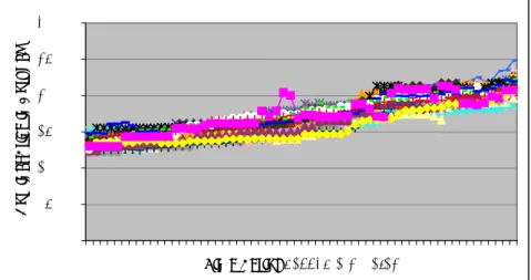
Engel and Rogers (2001) argued that their results are to a large extent explainable by stickiness of prices. We also - in Figure 9 - depict the relationship between the deviation of the relative LOOP (the denominator of the k

i

r coefficient) and the stickiness of prices as measured by the standard deviation of the nominal price of each individual good across all districts. The correlation between these two series is 0.763, and the positive relationship is clearly seen in Figure 9. The smaller the standard deviation of the nominal price, the smaller the denominator of the k

i

r coefficient.

20 _{Herrmann-Pillath (2001, p. 55) comments in this respect. “Engel/Rogers (1999) show that relative-relative} price movements seem to manifest a violation of the LOP for tradables, and just the opposite for non-tradables which flies in the face of any sensible understanding of LOP.”

20

5

The speed of adjustment

In this Section we estimate the speed of adjustment of prices to the law of one price. As suggested by Parsley and Wei (1996), we start by estimating

( ) , , , , 1 , , , , 1 s k i k t i k t m i k t m i k t m q βq ₋ γ q ₋ ε = ∆ = +

∑

= , i is the benchmark district, j is the respective district, k is

com-modity, and t is the time period. In this section Bratislava and Banska Bystrica served as benchmark districts. These two cities provide a natural benchmark, Bratislava because of its importance as a political and economic capital of the country, and Banska Bystrica be-cause of its being another large city in the middle of the country.21 Our estimation proce-dure is based on the work of Levin and Lin (1992).

The findings in Section 3 show that there are large differences in nominal prices across districts. These differences may make the test of convergence as described in (4) somewhat unrealistic, since it does not account for any district-specific effect. For this reason, we per-form the panel unit root analysis also for de-meaned data as follows.

( ) , , , , 1 , , , , 1 s k i k t i k t m i k t m i k t m q βq − γ q − ε = ∆% = % +

∑

∑

Thus while (4) informs us on the absolute LOOP, (5) speaks to the speed of convergence to the relative LOOP. In both specifications, the main parameter of interest is β, related to the speed of convergence. Under the null hypothesis of no convergence, β is to equal to zero, meaning that shocks to q_{i k t, ,} are permanent. Convergence implies a negative value of β,

with the approximate half-life of a shock given by ln 2

ln(1 β)

−

+ .

21 _{The last natural option for the benchmark city would be Košice, because of its size and economic} impor-tance. We opted against Košice as a benchmark because of its geographical location on the very east of the country. We believe that Bratislava and Banska Bystrica represent the only natural choice for benchmark district, and while the convergence results may not be invariant to the choice of benchmark, choosing another benchmark city would not make much sense from the economic point of view.

21

We perform the analysis for 157 non-perishable final products, 49 perishable products and 24 services. These products are listed in Tables 8-10, with Bratislava serving as bench-mark. These tables display the β coefficients from equations (4) and (5). To obtain the auto-regressive coefficient, one would need to add one to the value of β. The closer the es-timate of β to zero, the longer the estimated half-life of a disturbance and the more likely it is that the data contain a unit root.

In Table 7 we report the summary of the results for the sample of non-perishable goods, perishable goods and services. The adjustment among Slovakian cities is slower for non-perishable goods and for services than the corresponding results obtained in Parsley and Wei (1996) for the respective groups of products, 15.84, 12.18 and 46.21. However, adjustment is faster for perishable goods not depending on the benchmark.

Median values for the half-life of price convergence are considerable lower if we use specification (5). We also note that the β coefficient using specification (4) is positive in 34 out of 157 cases for non-perishable goods, 6 out of 49 cases for perishable goods and 8 out of 24 cases for services. However, using specification (5), the β coefficient is always nega-tive and the presence of the unit root is rejected in all cases.

Finally, we calculate the mean log-difference for all the commodities and regress it on the distance to the benchmark and the size of the individual city. We control for non-linearity by adding quadratic terms. The results are presented in Tables 11 and 12. These results show that the size variable is an important determinant of the level of mean log-differences in prices. It has a negative coefficient and is almost always statistically signifi-cant, except for a couple of cases where the quadratic terms are added. This means that the higher the population of the main city in the district, the higher the level of prices. The quadratic term of population is almost always statistically insignificant. The distance from the benchmark district does not seem to be a determinant, except for the nonperishable commodities group with the benchmark district Bratislava.22

22 _{One may suggest the following explanation. First, non-perishable goods can be easily transported and} therefore produced only at a couple of locations in a country (unlike perishable goods). Second, economic activity, which is greater in the western part of Slovakia, seems to be an important determinant of equilibrium price level. With Bratislava being in the most western part of Slovakia, the distance variable works as a proxy for the level of economic activity.

22

6

Conclusions

This paper uses a large panel data set for final goods and services across 38 Slovakian dis-tricts over the period 1997:01-2001:12 to examine the nature of deviations from the law of one price in the context of the small transition economy. In this paper we provide three type of investigations. First, we document the range of price differences across Slovak dis-tricts. Second, we find that the variability of relative prices in the same district is higher than the variability of the prices of the same good across different districts. We investigate the factors, which may be deemed responsible for this finding. Third, we investigate the speed of convergence to the LOOP in the spirit of Parsley and Wei (1996). We find evi-dence for convergence; however its speed - while faster than typically found in cross-country data - is lower than that found for the US cities. The speed of convergence in panel unit root tests increases considerably if we condition on district-specific factors by using de-meaned relative price data.

23

References

Cecchetti, Stephen G., Nelson C. Mark and Robert Sonora, (2000), “Price Level Conver gence among United States Cities: Lessons for the European Central Bank,” National Bureau of Economic Research, Working Paper 7681, May 2000

Conway, Patrick, (1999) “Privatization and Price Convergence: Evidence from Four Markets in Kyiv,” Journal of Comparative Economics, 27 2, pp. 231-57

Cushman, David O., Ronald MacDonald, and Mark Samborsky, (2001) “The Law of One Price for Transitional Ukraine,” mimeo, May.

Engel, Charles (1993), “Real Exchange Rates and Relative Prices, An Empirical Investiga tion,” Journal of Monetary Economics, 32, pp. 35-50

Engel, Charles, and John H. Rogers, (1996), “How Wide is the Border,” The American Economic Review, Vol. 86 No.5, pp. 1112-1125

Engel, Charles and John H. Rogers, (2001) “Violating the Law of One Price: Should We Make a Federal Case Out of It?” Journal of Money, Credit and Banking, Vol. 33., No.1 Haskel, Jonathan and Holger Wolf, (2001) “The Law of One Price - A Case Study,”

Work-ing Paper, National Bureau of Economic Research, February, WorkWork-ing Paper 8112 Herrmann-Pillath, Carsten, (2001) “A General Refutation of the Law of One Price as Em

pirical Hypothesis”, Jahrbucher fur Nationalokonomie und Statistik, Vol. 221/1, pp. 45-67

Imbs Jean, Haroon Mumtaz, Morten O. Ravn, and Helene Rey, (2002), “PPP Strikes Back: Aggregation and the Real Exchange Rate,” National Bureau of Economic Research, December, Working Paper 9372

Kárász, Pavol, Pavol Kárász jr. and Radovan Pala (2000), “Development Possibilities of Regions of the Slovak Republic,” Friedrich Ebert Stiftung, March, mimeo

Levin, Andrew and Chien-Fu Lin, (1992), “Unit Root Tests in Panel Data: Asymptotic and Finite-Sample Properties,” University of California, San Diego, Department of Eco nomics, Discussion Paper 92-23

O’Connel, Paul G.J. and Shang-Jin Wei, (2002), “”The Bigger They Are, the Harder They Fall”: Retail Price Differences across U.S. Cities,” Journal of International Economics, 56, pp. 21-53

Parsley, David C. and Shang-Jin Wei, (1996) “Convergence to the Law of One Price with out Trade Barriers or Currency Fluctuations,” The Quarterly Journal of Economics, November pp. 1211-1236

Ratfai, Attila (2003), “Inflation and Relative Price Asymmetry,” Central European Univer-sity, Department of Economics, mimeo

Wei, Xiangdong and C. Simon Fan, (2002) “Convergence to the Law of One Price in China,” mimeo

Vidovic, Stanislav, (2003) “Convergence of Prices to the Law of One Price in Slovakia,” MA thesis, Central European University, Department of Economics

24

World Bank (2002), “Slovak Republic Development Policy Review,” November, Main Report, Poverty Reduction and Economic Management Unit, Europe and Central

25

Table 1: Basic relative prices of selected final goods and service across Slovak districts Product Maximum to Minimum

Relative Price Ratio Relative Price Ratio Maximum to Mean of Variation Coefficient

Rice 1.697 1.465 0.091 Sugar 1.192 1.087 0.034 Potato 1.854 1.366 0.141 Milk 1.302 1.160 0.057 Butter 1.254 1.145 0.052 Eggs 1.365 1.183 0.068 Oranges 1.398 1.214 0.077 Poppy Seed 1.589 1.115 0.077 Cheese 'Niva' 1.237 1.098 0.047 Wheat Flour 1.348 1.149 0.065 White Roll 1.630 1.244 0.114 White Bread 2.012 1.698 0.140 Oat Flakes 1.402 1.203 0.078

Boneless Chunk Roast 1.340 1.120 0.067 Boneless Beef Rear 1.369 1.150 0.069 Boneless Pork Shoulder 1.224 1.113 0.049 Chicken Fryer 1.208 1.106 0.039 Ham Salami 1.214 1.081 0.040 Coffee 1.566 1.200 0.091 Lentilky Candies 1.211 1.108 0.039 Cigarette ‘Dalila’ 1.179 1.041 0.029 Cigarette ‘Mars’ 1.098 1.051 0.024 Vlassky Salad 1.600 1.296 0.111 Alpa Francovka 2.250 1.363 0.128 Linen Bed Sheet 1.405 1.179 0.070 Lady's Stockings 3.232 2.367 0.353 Men’s Sports Leather Shoes 2.266 1.542 0.256 Wooden Coffin 3.076 1.724 0.224

Matches 1.511 1.313 0.092

Children Game 2.551 1.198 0.155 Men’s Boxer Shorts 2.399 1.821 0.227

Cement 1.273 1.113 0.058

Gasoline 91 1.031 1.010 0.006 Cover Sheet Larisa 1.498 1.270 0.091 Storage Cane 'Omnia' 1.495 1.251 0.093 Meal in Restaurant – Schnitzel 1.861 1.262 0.136 Wedding Dress Borrowing 2.304 1.347 0.192 Drivers License Fee 1.633 1.315 0.115 Videotape Borrowing 1.986 1.375 0.159 Apartment Rent 2 Bedrooms 3.406 1.377 0.203 Apartment Rent 3 bedrooms 2.625 1.136 0.138 Apartment Rent – Services 6.109 2.257 0.422 Apartment Painting 5.424 2.150 0.407 Classical Theater Ticket 7.415 2.045 0.460

Data are from April 2001. Results in Table 1 calculated from nominal prices expressed in Slovak korunas. Maximum (minimum) is the highest (lowest) price observed in any of the thirty-eight districts. If the static law of one price holds, our threshold would be 1.00 both for max-min as well as for max-mean ratios.

26

Table 2: Share of pairwise relative prices higher than one District Name Coefficient District Name Coefficient

Bratislava 74.67 Banská Bystrica 50.03 Bratislava-vicinity 49.96 Lučenec 51.79 Dunajská Streda 61.47 Rimavská Sobota 40.10

Galanta 43.11 Veľký Krtíš 41.92

Senica 51.41 Zvolen 40.72

Trnava 43.48 Žiar nad Hronom 42.17 Považská Bystrica 47.20 Bardejov 48.39

Prievidza 35.38 Humenné 41.79

Trenčín 49.71 Poprad 46.00

Komárno 49.34 Prešov 44.50

Levice 52.04 Stará Ľubovňa 43.05

Nitra 54.17 Svidník 46.13

Nové Zámky 54.74 Vranov nad Topľou 46.95 Topolčany 43.62 Košice 63.10 Čadca 42.30 Košice-vicinity 41.48 Dolný Kubín 52.37 Michalovce 48.58

Liptovský Mikuláš 62.22 Rožňava 53.80 Martin 50.09 Spišská Nová Ves 52.79

Žilina 54.61 Trebišov 50.09

Data for April 2001. Pairwise relative price calculated as a simple ratio of nominal prices for each product for two districts. Thus for each district this measure contains 2580 relative pairwise prices. Coefficient in the Table 2 provides a percentage value for the number of observations for which this relative pairwise price is higher than one.

Table 3: Description of data

Size Weight in CPI Weight in our sample T1: Bread, Cereals, Meat and Fish 45 106.0 168.31

T2: Milk, Cheese, Eggs, Oils and Fats 19 53.6 79.63 T3: Fruit, Vegetables and Other Food 58 54.1 85.29 T4: Beverages and Tobacco 21 92.0 150.76

T5: Clothing 61 54.3 59.13

T6: Footwear 12 20.7 28.10

T7: Housing, Water, Electricity, Gas 24 215.3 47.60 T8: Furnishings, Household Equipment and Maintenance 80 51.8 56.53

T9: Health 16 14.5 11.04

T10: Transport 31 125.5 106.41

T:11: Recreation and Culture 61 72.1 88.21 T12: Restaurants and Hotels Services 33 72.2 45.48 T:13: Personal Care 40 67.9 73.48

Total 501 1000.0 1000

Size: number of products in the sample in each group of products;

27

Table 4: The ratio of relative price variability across districts and cross-district variability of the relative law of one price deviations

k i

r (un) r_ik(w) r_ik<1 r_ik(un)12 r_ik(w)12 r_ik<1 (12) T1: Bread, Cereals, Meat and Fish 1.59 1.62 --- 1.99 2.14 --- T2: Milk, Cheese, Eggs, Oils and Fats 1.80 1.92 --- 2.25 2.45 --- T3: Fruit, Vegetables and Other Food 1.34 1.35 8 1.61 1.68 4 T4: Beverages and Tobacco 1.88 2.08 --- 2.32 2.79 --- T5: Clothing 1.39 1.33 1 1.29 1.21 4 T6: Footwear 1.34 1.32 ---- 1.20 1.18 --- T7: Housing, Water, Electricity, Gas 1.29 1.30 5 1.28 1.39 6 T8: Furnishings, Household Equipment

and Maintenance

1.46 1.52 6 1.34 1.40 11 T9: Health 1.83 1.88 1 2.67 2.84 1 T10: Transport 1.57 3.99 10 2.42 8.58 13 T:11: Recreation and Culture 1.25 1.24 7 1.13 1.12 15 T12: Restaurants and Hotels Services 1.52 1.39 2 1.39 1.52 3 T:13: Personal Care 1.44 1.51 --- 2.62 1.44 2

Total 1.47 1.86 40 1.59 2.59 59

k i

r (un): un-weighted average of the r_ikcoefficient; prices are measured as one-month log difference

k i

r (w): weighted average across the group of products of the r_ikcoefficient

k i

r <1: number of cases in the group where the coefficient was lower than one

k i

r (un)12: like r_ik(un) except that prices are measured as twelve-month log differences

k i

r (w)12: like r_ik(w) except that prices are measured as twelve-month log differences

k i

r <1 (12): number of cases in the group where the coefficient was lower than one.

Table 5: Measure of the relative law of one price

den (un) den (w) T1: Bread, Cereals, Meat and Fish 3.85 3.65 T2: Milk, Cheese, Eggs, Oils and Fats 3.94 3.73 T3: Fruit, Vegetables and Other Food 9.45 9.90 T4: Beverages and Tobacco 4.01 3.45

T5: Clothing 4.43 4.48

T6: Footwear 4.42 4.51

T7: Housing, Water, Electricity, Gas 5.68 5.78 T8: Furnishings, Household Equipment and Maintenance 4.23 3.95

T9: Health 4.36 4.70

T10: Transport 6.07 2.79

T:11: Recreation and Culture 5.28 5.56 T12: Restaurants and Hotels Services 4.20 3.63 T:13: Personal Care 4.38 4.13

Total 5.13 4.47

den (un): un-weighted average of the denominator of the r_ikcoefficient multiplied by 100 den (w): weighted average of the denominator of the r_ikcoefficient multiplied by 100

28

Table 6: Values based on division of products to tradables and non-tradables k

i

r den k

i

r den

Unweighted average Weighted average

Non-traded Goods 1.32 5.46 1.33 5.37

Traded Goods 1.50 5.07 1.93 4.35

Total 1.47 5.13 1.86 4.47

For explanation, see Tables 4 and 5.

Table 7: Half-life of price convergence in months

Specification (4) Specification (5)

Benchmark District

Bratislava Banska Bystrica Bratislava Banska Bystrica

Non-Perishable 29.56 21.81 5.68 5.24 Perishable 9.82 6.18 1.98 2.78 Services 79.62 49.35 7.34 6.40 Half-life calculated as ln 2 ln(1 β) −

+ . In the table we report the median value.

29

Table 8: Panel unit root test: non-perishable goods

Product β (4) Half-life β (5) Half-life

Rice 0.015 -46.041 -0.084 7.907

Wheat Flour Half-Fine 0.002 -310.605 -0.271 2.192

Farina 0.016 -44.407 -0.205 3.028

Wafers without Flavor -0.032 21.440 -0.228 2.677

Pasta -0.003 237.273 -0.091 7.280

Dough -0.078 8.508 -0.199 3.124

Oat Flakes without Flavor -0.029 23.534 -0.225 2.720 Dried Milk for Babies -0.149 4.305 -0.195 3.203 Dried Milk Half-Fat -0.037 18.138 -0.177 3.566 Dried Grapes 0.005 -146.725 -0.149 4.288 Peanuts Peeled Salted 0.008 -86.677 -0.092 7.146 Beans White Dried -0.010 68.480 -0.112 5.817

Lentils -0.029 23.236 -0.166 3.808

Soya Meat -0.028 24.315 -0.154 4.145 Sour Cabbage -0.024 28.415 -0.282 2.093 Peas in Salty Water -0.014 48.711 -0.186 3.371

Leco -0.023 29.206 -0.235 2.591

Granulated Sugar -0.066 10.201 -0.401 1.352 Ground Sugar -0.047 14.271 -0.361 1.550 Cooking Chocolate 0.004 -174.745 -0.268 2.221

Salt 0.008 -89.006 -0.216 2.842

Ground Sweet Paprika -0.019 36.176 -0.167 3.787 Ground Pepper -0.003 250.490 -0.217 2.827 Caraway not Ground -0.034 19.999 -0.146 4.379

Vinegar -0.060 11.138 -0.254 2.365

Baking Powder -0.126 5.152 -0.358 1.566 Cocoa Powder 0.057 -12.546 -0.163 3.885 Table Mineral Water -0.031 21.663 -0.044 15.243 Fruit Sirup -0.025 27.369 -0.195 3.201 Rum 38-40% 0.001 -721.684 -0.203 3.048 Vodka 38-40% -0.022 30.830 -0.111 5.896 Brandy 38-40% -0.002 424.387 -0.147 4.360 Wine Red Bottled -0.021 32.746 -0.245 2.468 Wine White Bottled -0.020 34.174 -0.159 4.006 Wine Sparkling 0.027 -25.837 -0.304 1.910 Cotton Dress Material for Ladies -0.021 32.577 -0.084 7.904 Ladies Synthetic Dress Material -0.010 71.390 -0.099 6.677 Ladies Woolen (Partly) Dress Material -0.007 102.763 -0.108 6.046 Short Underwear for Men 0.000 -6078.16 -0.098 6.712 Long Underwear for Men -0.006 122.495 -0.150 4.250 Undershirt for Men 0.008 -83.127 -0.132 4.908 Pyjamas for Men 0.007 -98.983 -0.096 6.864 Shorts for Men 0.019 -37.061 -0.079 8.417 Men Bathroom Gown -0.045 14.995 -0.099 6.637 Panties for Women -0.005 134.331 -0.082 8.094 Night Dress for Women 0.006 -115.318 -0.104 6.315 Underwear for Women 0.008 -88.940 -0.121 5.355 Pyjamas for Women -0.013 51.032 -0.196 3.186

Bra -0.013 51.326 -0.079 8.416

Home Dress for Women -0.020 34.039 -0.099 6.642

30

Continued Table 8

Product β (4) Half-life β (5) Half-life Shirt for Babies -0.045 14.965 -0.099 6.654 Cotton Napkins for Babies -0.038 18.055 -0.179 3.517 Short Sleeved Shirt for Children -0.011 60.936 -0.118 5.517 Panties for Girls 0.004 -158.048 -0.115 5.678 Underwear for Boys 0.003 -210.946 -0.074 8.989 Pyjamas for Children -0.011 63.033 -0.180 3.485 Undershirt for Children 0.009 -78.412 -0.104 6.307 Long Winter Coat for Men -0.044 15.499 -0.135 4.796 Winter Jacket for Men -0.019 35.788 -0.143 4.485 Baby Stockings -0.019 36.439 -0.066 10.109 Ladies Stocking -0.001 594.060 -0.088 7.486 Socks for Children 0.005 -130.492 -0.123 5.283 Stockings for Children -0.014 50.423 -0.126 5.148 Handkerchief for Women 0.003 -230.991 -0.071 9.480 Knit Cap for Children -0.008 90.625 -0.066 10.124 Knit Gloves for Children -0.023 29.563 -0.046 14.872 Knit Thread -0.014 50.110 -0.150 4.267 Rubber Strap -0.020 34.015 -0.095 6.967 Metal Zipper -0.030 22.703 -0.097 6.818 Repair of Heels for Women -0.013 51.570 -0.081 8.210 Latex Paint Universal -0.076 8.727 -0.082 8.128

Paint -0.102 6.445 -0.215 2.859

Basic Synthetic Paint -0.008 85.677 -0.064 10.476 Synthetic and Oil Paint -0.060 11.149 -0.180 3.489 Cement SPC 325 -0.032 21.071 -0.236 2.580

Lime -0.008 88.388 -0.143 4.502

WC Bowl with Flusher 0.006 -121.781 -0.071 9.450 Painting Services -0.013 53.765 -0.068 9.844 Painting of Wooden Products -0.016 43.338 -0.055 12.358

Propan-Butan -0.047 14.421 -0.358 1.565

Curtains -0.003 212.155 -0.058 11.677

Bed Sheet -0.003 219.648 -0.111 5.876 Bed Linen for Children 0.000 2063.035 -0.120 5.402 Bed Linen for Adults 0.000 3679.961 -0.099 6.619 Turkish Towel 0.002 -319.224 -0.095 6.925 Table Cloth 0.009 -79.517 -0.083 8.037 Dish Cloth 0.002 -292.052 -0.135 4.790 Synthetic Cover Larisa -0.001 624.599 -0.091 7.288 Comforter, Synthetic Material 0.031 -22.429 -0.047 14.515 Quilt Feather Filling -0.016 44.105 -0.117 5.558 Glass without Holder -0.023 29.754 -0.102 6.410 Crystal Glass Leaden with Holder -0.013 54.796 -0.083 7.999 Plate Set for 6 People -0.003 260.687 -0.119 5.480 Porcelain Cup with Decorations -0.022 31.082 -0.078 8.515 Glass Bowl from Silex with Cover -0.027 25.750 -0.129 5.002 Thermos with Pump 1 Liter -0.006 108.706 -0.135 4.766 Kitchen Pot 4 Liters 0.007 -96.760 -0.114 5.739 Tea Kettle 0.004 -197.772 -0.057 11.841 Cutlery for 6 Persons -0.021 33.306 -0.038 17.877 Kitchen Knife with Plastic Handle -0.010 68.567 -0.100 6.604

This table lists 51-100 products and is continued in the next page.

31

Table 8 Continued

Product β (4) Half-life β (5) Half-life Soup Ladle – Rustles -0.006 118.677 -0.096 6.874 Infant Bottle from Plastic -0.029 23.207 -0.262 2.286 Kitchen Scales 0.007 -101.393 -0.067 10.021 Wooden Ladle -0.011 61.673 -0.146 4.380 Plastic Bucket -0.006 116.571 -0.105 6.244 Flat Light Switch -0.022 31.080 -0.082 8.078 Electric Adapter -0.019 35.992 -0.097 6.803 Regular Light Bulb 0.007 -92.879 -0.123 5.276 Roll-on Meter -0.006 124.797 -0.066 10.179 Combination Pliers -0.002 312.137 -0.065 10.238 Screw Driver -0.020 34.990 -0.101 6.493 Metal Rake without Handle -0.067 9.947 -0.204 3.040 Aluminum Double Ladder -0.019 35.323 -0.121 5.354 Household Scissors -0.019 35.861 -0.102 6.464 Drier for Laundry -0.106 6.161 -0.133 4.848 Ironing Board -0.016 43.976 -0.103 6.408 Construction Nails -0.007 95.893 -0.104 6.281

Chamomile -0.082 8.086 -0.251 2.397

Herb Tea -0.096 6.881 -0.156 4.091

Thermometer -0.077 8.647 -0.149 4.283

Adhesive Plaster in a Pack -0.039 17.447 -0.192 3.256 Bandage Material -0.048 14.077 -0.168 3.776 Protection Means -0.004 165.714 -0.088 7.561 Disk Brake Slabs -0.009 80.105 -0.072 9.334

Accumulator -0.003 211.088 -0.074 8.985 Halogen Light Bulb -0.004 184.421 -0.060 11.113

Gasoline 91 Octane -0.540 0.892 -0.719 0.547 Gasoline 95 Octane -0.222 2.760 -0.391 1.399 Oil Fuel -0.441 1.192 -0.723 0.539 Motor Oil -0.002 302.862 -0.048 13.997 Gear Box Oil -0.005 139.864 -0.072 9.324 Non-Freezing Liquid for Cooler -0.023 29.734 -0.087 7.582 Electronic Pocket Calculator 0.007 -99.376 -0.082 8.124 Ball for Children -0.072 9.245 -0.106 6.170 Clovece Nehnevaj Sa -0.006 110.496 -0.153 4.185 Plastic Bob Sled with Brakes -0.038 18.030 -0.114 5.727

Volleyball -0.006 120.482 -0.124 5.229

Videotape – Clean -0.026 26.362 -0.058 11.551 Tape for Sound Recording – Clean -0.018 38.837 -0.142 4.520 Colored Postcard -0.013 55.084 -0.074 9.025 Spiral Calendar -0.035 19.469 -0.109 6.006 Notebook – Halfthick 40 Sheets -0.076 8.806 -0.139 4.614 Note Book A4 -0.012 57.070 -0.098 6.706 Black Pencil -0.004 173.537 -0.121 5.374 Celluloid Ruler -0.018 38.597 -0.110 5.932 Design A4 -0.026 26.442 -0.144 4.447 Color Pencils -0.014 48.196 -0.124 5.258 Razor Blade – 5 Pieces in a Pack 0.002 -353.988 -0.055 12.303 Francovka Alpa – Cosmetic Alcohol -0.007 94.006 -0.135 4.777 Folded Bandage Absorbant Cotton -0.047 14.491 -0.149 4.290

32

Continued Table 8

Product β (4) Half-life β (5) Half-life Paper Handkerchiefs 10

Pieces

-0,003 247,008 -0,047 14,257 Toilet Paper 400 Slips 0,002 -315,891 -0,116 5,602 Paper Napkins -0,003 274,748 -0,121 5,356 Umbrella for Women -0,016 42,191 -0,087 7,623 School Bag -0,016 44,070 -0,105 6,252

Matches -0,009 77,469 -0,195 3,201 Wooden Coffin -0,001 478,826 -0,057 11,859

Table 8 lists 157 products; the benchmark district for this data is Bratislava.

β (4) is the coefficient from equation (4).

β (5) is the coefficient from equation (5). Half-life in both cases calculated as ln 2

ln(1 β)

−

33

Table 9: Panel unit root test: perishable goods

Product β (4) Half-life β (5) Half-life Rye Bread 0.000 -1510.71 -0.111 5.911 White Roll -0.045 15.148 -0.107 6.136 Christmas Cake 0.003 -255.313 -0.131 4.928

Dumplings -0.022 31.265 -0.133 4.838

Chunk Roast with the Bone -0.020 34.771 -0.244 2.473 Boneless Chunk Roast -0.035 19.253 -0.284 2.075 Beef Rear Boneless -0.037 18.445 -0.339 1.675 Pork Meat with Bone -0.112 5.858 -0.428 1.241 Pork Neck with Bone -0.005 151.484 -0.426 1.247 Pork Side -0.131 4.946 -0.462 1.117 Pork Leg Boneless -0.083 7.960 -0.416 1.288 Pork Shoulder Boneless -0.140 4.594 -0.467 1.103 Chicken Fryer -0.081 8.220 -0.295 1.984 Chicken Portioned -0.044 15.300 -0.338 1.683 Diet Salami Pork -0.027 25.446 -0.200 3.106 Stewed Ham Pork -0.027 24.964 -0.227 2.696 Smoked Bacon with Skin 0.004 -187.37 -0.030 23.090 Fish Fillet not Breaded -0.033 20.929 -0.266 2.238 Smoked Fish -0.072 9.233 -0.172 3.679 Fish Salad with Mayonnaise -0.058 11.659 -0.144 4.469 Half-Fat Milk -0.015 45.728 -0.172 3.673 Sweet Cream -0.048 14.015 -0.121 5.385 Sour Cream -0.068 9.820 -0.144 4.462 Sheep Cheese -0.005 132.309 -0.243 2.489 Cheese Edam -0.027 25.362 -0.356 1.573 Eggs -0.020 33.572 -0.447 1.169 Fresh Butter -0.008 83.203 -0.282 2.089 Oil 0.023 -30.941 -0.163 3.897 Pork Lard -0.032 21.137 -0.156 4.087 Oranges -0.054 12.530 -0.762 0.483 Lemons -0.120 5.430 -0.546 0.877 Kiwi -0.244 2.474 -0.619 0.719 Banana -0.363 1.537 -0.832 0.388 Celery -0.211 2.917 -0.544 0.882 Carrot -0.183 3.439 -0.321 1.791 Parsley -0.206 3.005 -0.773 0.467 Cabbage -0.082 8.149 -0.531 0.914 Salad Cucumber -0.578 0.804 -0.985 0.165 Pepper -0.171 3.699 -0.790 0.444 Onion -0.187 3.347 -0.240 2.523

Vegetable Mixed Frozen -0.014 48.806 -0.101 6.496 Spinach Stew Frozen -0.045 14.993 -0.461 1.121

Potato -0.124 5.216 -0.674 0.618 Fresh Yeast -0.004 175.689 -0.054 12.600 Garlic -0.183 3.432 -0.343 1.652 Beer 10% Bottled 0.016 -42.477 -0.081 8.230 Beer 12 % Bottled 0.003 -210.59 -0.155 4.124 Karafiat -0.023 29.149 -0.356 1.575 Rose -0.052 12.863 -0.309 1.877