A STUDY ON AGENT SCHEDULING SCENARIOS IN
MULTI-AGENT SYSTEMS
1
CECILIA E. NUGRAHENI, 2LUCIANA ABEDNEGO
1,2
Department of Computer Science, Parahyangan Catholic University, Indonesia
E-mail: [email protected], [email protected]
ABSTRACT
A multi-agent system (MAS) is understood as a collection of intelligent agents that interact with each other and work together to achieve a goal. Since it consists of many agents, the communication, coordination, and scheduling among agents are important issues in MAS. This paper presents a study on the effect of agent scheduling on the performance of a MAS. The study is conducted on a small parameterized MAS, which is a Sudoku solver. Four agent scheduling scenarios have been developed and implemented. Some experiments have been conducted to measure the performance of each scenario. It is shown that the scheduling scenarios have effect on the system performance.
Keywords: Multi-Agent Systems, Agent Scheduling Scenario, Sudoku, Sudoku Solver, Block World Problem
1.
INTRODUCTIONMulti-Agent Systems (MAS) has become one of popular paradigms for understanding and building complex systems, especially distributed systems [1, 2]. This paradigm is widely used to develop nowadays systems. It has been applied in various fields, e.g. in health and medical [3,4], traffic and transportation [5,6], etc.
A MAS is understood as a collection of intelligent agents that interact with each other and work together to achieve a goal. In this context, the agents are software or computer programs. Since it consists of many agents, the communication, coordination, and scheduling among agents are important issues in MAS.
This work focuses on an important issue of MAS which is scheduling. The objective of this research is to analyze the effect of scheduling scenario on the performance of a MAS. By knowing the effect of the agent scheduling scenarios, we can apply an appropriate or optimal scheduling scenario in order to get the best performance of a MAS.
Various reviews on MAS can be found in literature, ranging from the aspect of architecture, agent communication, agent scheduling, modeling, verification, performance, and application of MAS. In particular, there are many research related to performance evaluation of MAS, e.g. performance comparison of two information retrieval MAS: the one contains stationary agents only and the other
contains one mobile agent [7], performance comparison between two MAS for combinatorial auction and voting with different architecture and agent communication [8], comparative study of two different open-source MAS architectures [9], and comparison between centralized and decentralized scheduling approach of MAS [10]. Similar to [10], this work focuses on the effect of scheduling algorithm on the performance of MAS.
As case study we took MAS-based Sudoku solver [11,12]. A research related to MAS that also used Sudoku as the case study is found in [13]. However, the modelling of Sudoku in [13] is different from our model. We use BWP-based Sudoku Solver that, in our knowledge, has been never used before by other researchers.
We limited our work on a class of MAS which is parameterized MAS. This makes the difference between this work and the others. The underlying concept of parameterized MAS is parameterized systems proposed in [14]. More work related to parameterized systems can be found in [15,16,17]. We also limit our work to the interleaving systems which means that at every time there is maximum one active process.
study like Sudoku puzzle can be used to study
complex systems.
The rest of this paper is structured as follows. Section 2 explains the concept of BWP and how to model Sudoku Solver as BWP. Section 3 presents our BWP-based Sudoku solver that we used for the case study. Section 4 and section 5 describes the scheduling scenarios and the experimental results, respectively. Conclusion and future work are given in Section 6.
2.
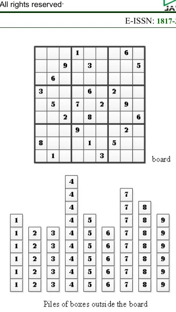
MODELLING SUDOKU PUZZLES AS BWPS [image:2.595.316.493.94.408.2]A BWP consists of a set of blocks, a table, and two robots. The blocks are initially arranged in some vertical stacks. Each robot has its own task capability: the first robot is capable to take a box at a top of a stack and put it on the table, whereas the second robot is capable to take a box on a table and put it on a top of a stack. The problem is how to change the initial arrangement to a new different arrangement by using the two robots. Several approaches for modelling and solving BWP can be found in literature, for example in [18]. An illustration of a BWP is given in Figure 1.
Figure 1. A Block World Problem.
BWP is frequently used in explaining the concept of Multi-Agent Systems. In particular, in [17] BWP is used as a case study for formal modelling and verification of parameterized MAS. A parameterized MAS is a MAS consisting a number of similar agents. The number of the agents is given as parameter of the system. It is assumed that the system is interleaving, that means there is only one agent works at a time.
[image:2.595.91.291.440.529.2]Inspired by [17], we have proposed a novel approach for solving Sudoku puzzles, which is by modelling Sudoku puzzles as BWPs [11]. By modifying some settings of block world problem we have shown that Sudoku puzzles can be regarded as a variant of BWP. The modification is illustrated in Figure 2.
Figure 2. Modification of a BWP.
Three models for BWP based Sudoku solver have been defined in [11]. The difference among the models lies on the number and the task or the capability of the robot.
The first model uses two robots and is based on backtracking principle. This model is very similar to the original BWP. The first robot’s task is to take a box and tries to put on a cell on the board which is valid for the box. Whereas the second robot’s task is to take a box from a cell and put it back to the stack outside the board. The first robot gets the first turn, repeatedly does it task until all cells are filled with boxes or it is unable to find a box that can be placed on an empty cell. If the last condition holds, then the second robot will do its task by taking the last box put by the first robot from the board. The searching for a solution is then continued. Given a valid Sudoku puzzle, model 1 guarantees that a solution will be found.
box with number i on that cell. After doing its job,
the robot i will give the turn to the next robot. After the robot 9 does its job, it will be decided whether a new iteration should be made or not. If in the last iteration, all the robots cannot find appropriate cells, then the process is stopped. Differs from the first model, the second and the third model cannot guarantee to find a solution for a, even, valid puzzle.
Later, a new Sudoku Solver model has been proposed [12]. All four models have been successfully implemented and tested on 100 Sudoku puzzles. The experimental results show that the first model provides the best performance, followed by the fourth model. It is also reported that the combination of model 4 and model 1 gives improvement to the performance of the Solver.
In [12] all the models apply the same agent scheduling scenario. In this work, we will study the effect of agent scheduling on the performance of the Sudoku Solver. For that purpose, we define four scheduling scenarios. We apply each scenario on the fourth model. Experiment will be conducted to measure the performance of each scenario. We then compare the performance of each scenario with the original scenario.
3.
BWP-BASED SUDOKU SOLVERA Sudoku puzzle can be viewed as a BWP whose elements are a table, a board, a set of boxes and a set of robots [11,12]. The board comprises of 3x3 sub-blocks, each sub-block is a 3 x 3 cells, and is located on the table. The number of the boxes is 9x9. Each box is labeled with a number within 1 to 9. For each label there are 9 boxes labeled with this number. The initial arrangement is the arrangement of the boxes so that there are some boxes are already put on the cells of the board and the rest of the boxes are outside the board. The boxes outside the board are organized in piles according to their numbers. The final arrangement is the arrangement of the boxes satisfying these conditions: all boxes are on the cells of the board, there are no boxes with the same label in the same row, the same column, and the same sub-block.
In this work, we used the fourth model proposed in [12]. Nine robots with the same capability are used by this model. Each robot is identified with a number from 1 to 9. Every robot is responsible to the stack of boxes according to its identifier. The task of the robots is to take a box from their corresponding stacks and put the box on a cell with
valid position of the board. A valid cell is defined as follows:
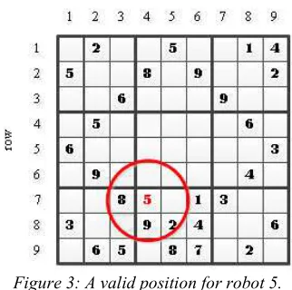
Definition 1 A robot i will call a cell at (x, y) a valid position if all the following conditions hold: 1) It is empty.
2) The row x does not contain any boxes with number i.
3) The column y does not contain any boxes with number i.
4) The sub-block where (x, y) is located does not contain any boxes with number i.
5) For every other row r in the same sub-block there is a box with number i or all cells in row r in the same sub-block with the cell (x, y) are not empty or the cell at the position (r, y) is not empty.
6) For every other column c in the same sub-block there is a box with number i or or all cells in column c in the same sub-block with the cell (x, y) are not empty or the cell at the position (x, c) is not empty.
[image:3.595.325.486.427.587.2]For example, Figure 3 illustrates a valid position for robot 5.
Figure 3: A valid position for robot 5.
To solve a puzzle, the solution searching process is done iteratively. At each iteration, the robots work one by one, in ascending order, starting from robot 1. Every time there is only one robot that works. In our implementation, a special module, called scheduler, is used to control this mechanism.
4.
SCHEDULING SCENARIOSagent is always the same, from 1 to 9. The
searching process is stopped whenever at an iteration all robots fail to do their tasks.
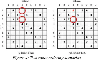
[image:4.595.307.503.195.266.2]By analyzing the fourth model, we can conclude that there are interdependencies among the robots in doing their tasks. Let’s consider the Sudoku puzzle in Figure 4 and focus on the upper middle sub-lock. Now assume that at an iteration, the robot 3 gets its turn before the robot 8. At this situation, the robot 3 cannot do its task successfully. There are two possible cells that can be taken, which are (1,4) and (3,4). However, the robot 3 has no capability to choose one of them due to the definition of valid position. The situation will be different if the robot 3 gets its turn after robot 8. Since robot 8 manages to put a box on cell on (1,4), therefore robot 3 can put a box on cell (3,4).
Figure 4: Two robot ordering scenarios
Based on the analysis, we draw a hypothesis that the agent ordering may bring effects on the performance of the Solver.
Since our focus is on the ordering of the robots, we define four scheduling scenarios that use random ordering principle. The first scenario (S1) and the second scenario (S2) are very similar to the original scenario (OS). Each scenario is described as follows:
• First scenario – S1
This scenario is very similar to OS, except before the first iteration, the scheduler generates an arbitrary permutation of a set {1, .., 9}. This permu-tation is then used as the ordering of agents. The algorithm is given in Figure 5.
ordering <- permutation(1,9) repeat
res <- false for (i in 1..9) do
res <- res or action(ordering[i]) endfor
until not res
Figure 5: S1 Algorithm. • Second scenario – S2
This scenario is very similar to OS, except before
every iteration, the scheduler generate an arbitrary permutation of a set {1, …, 9}. This permutation is then used as the ordering of agents. The algorithm is given in Figure 6.
repeat
ordering <- permutation(1,9) res <- false
for (i in 1..9) do
res <- res or action(ordering[i]) endfor
until not res
Figure 6: S2 Algorithm.
For the third (S3) and the fourth (S4) scenarios, at any iteration the scheduler picks a robot randomly. The searching process will be stopped whenever a stopping condition is reached. The difference between the both scenarios is on the stopping condition.
• Third scenario – S3
The stopping condition for S3 is defined as a condition when after a number of consecutive iteration there is no robot that can do its task successfully. As consequence, the scheduler has to record the number of failures. This number is reset whenever a successfully do its task. The algorithm is given in Figure 7.
counter <- 0
while (counter < max) do
i <- pick_one_robot_randomly() if (action(i)) then
counter <- 0 else
counter <- counter + 1 endif
endwhile
Figure 7: S3 Algorithm.
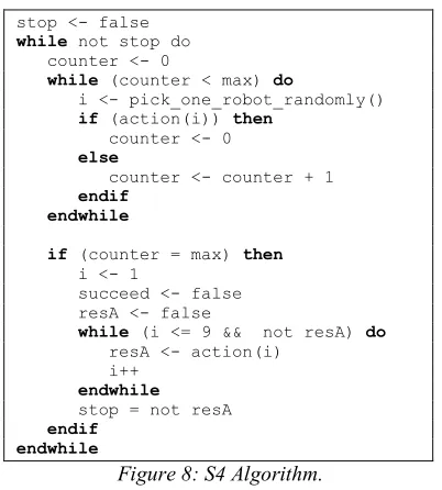
• Fourth scenario – S4
S4 is an improvement of S3. The improvement is done by adding a process after the stopping condition for S3 is reached. Before stopping the process, scheduler will ask every robot to do its task, from robot 1 to robot 9. If there is a robot doing its task successfully, the searching process is continued. The algorithm is given in Figure 8
5.
EXPERIMENTAL RESULTS [image:4.595.93.295.333.457.2]in [12]. Since each scenario contains a randomness
factor, for each scenario we run the Solver 9 times for each puzzle. For S3 and S4, we set max to 20.
stop <- false while not stop do counter <- 0
while (counter < max) do
i <- pick_one_robot_randomly() if (action(i)) then
counter <- 0 else
counter <- counter + 1 endif
endwhile
if (counter = max) then i <- 1
succeed <- false resA <- false
while (i <= 9 && not resA) do resA <- action(i)
i++ endwhile stop = not resA endif
[image:5.595.304.507.154.662.2]endwhile
Figure 8: S4 Algorithm.
[image:5.595.89.290.179.402.2]Our first experiment is to measure the average time needed by the Solver with a particular scenario in solving a Sudoku puzzle. From 100 puzzles, each scenario is only capable of solving 44 puzzles. This is the same number and the same puzzles that can be solved by OS. Without considering the puzzles that cannot be solved, the average time for solving a puzzle are shown in Table 1. We can see that S1 has the minimum average time, followed by S2, OS, S3, and the last is S4.
Table 1. Average Time for Solving a Puzzle
No OS S1 S2 S3 S4
1 8656 9920 9743 14994 15460
2 8469 9087 7831 12468 14058
3 13657 12392 11644 16949 17774
4 8500 8573 7465 12221 13951
5 10125 8964 8702 13572 14407
6 11203 9738 9724 13337 15593
7 8250 7767 8611 11234 14551
8 11109 10210 10137 15210 15048
9 12406 10925 10493 16435 15661
[image:5.595.88.291.560.719.2]10 11266 8936 10853 14830 14084
Table 1. Average Time for Solving a Puzzle (cont.)
No OS S1 S2 S3 S4
11 8578 8071 11248 12596 14259
12 12422 11818 11542 15102 18108
13 9984 8052 11841 14753 14247
14 9906 9196 12267 13813 14979
15 8750 9161 11965 13106 14634
16 9860 9561 7823 14112 15020
17 12453 10182 8514 15049 15996
18 9890 9443 8925 12493 13988
19 9797 9238 9345 13493 13616
20 12063 10570 9821 14717 15734
21 16218 13918 16934 18372 19457
22 20093 15606 19307 15540 21804
23 15391 15017 17423 17907 19278
24 26875 14455 19866 24063 27181
25 18421 12856 17151 23121 20797
26 19938 15055 19077 27486 17774
27 12031 10818 13106 18422 17742
28 18781 13277 14967 19716 17160
29 17344 14002 14920 22904 21692
30 18625 15939 18339 25142 23612
31 17813 13398 19403 25781 24819
32 21282 17644 20047 25894 21761
33 16187 12779 16488 27276 22672
34 15657 13471 14312 21136 20963
35 24860 19885 21119 24141 24272
36 11844 9975 12774 17541 16421
37 50578 13272 15984 23656 19248
38 13703 11147 12780 19065 17249
39 13578 11894 13477 17170 19400
40 15579 17217 17001 23245 25805
41 15016 13858 14769 16941 17817
42 12328 11325 12170 15386 15987
43 16750 22077 21932 21994 26351
44 11937 10890 11295 13369 16121
Average 14561 11813 13181 17457 17961
Table 2. Minimum Average Time
Scenario min. average time (times)
OS 4
S1 27
S2 12
S3 1
S4 0
The algorithm of S4 is more complex than the other scenarios, as predicted, S4 provides the worst performance in this experiment. For S3, from 9 attempts for solving a puzzle, it not always the case that all attempts succeed. The worst case is from 9 attempts, there are only two attempts that succeed.
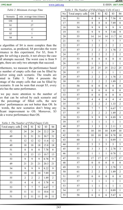
Furthermore, we measure the performance based on the number of empty cells that can be filled by the Solver using each scenario. The results are presented in Table 3. Table 4 presents the percentage of the empty cells that can be filled by each scenario. It can be seen that except S3, every scenario has the same performance.
[image:6.595.89.506.437.769.2]If we pay more attention to the number of puzzles that can be solved by each scenario and also the percentage of filled cells, the new scenarios’ performances are not better than OS. In other words, the new scenarios don’t bring any significant improvement to OS. Moreover, S3 provide a worse performance than OS.
Table 3. The Number of Filled Empty Cells
No Total emp ty cells OS S1 S2 S3 S4
1 52 24 24 24 22.2 24
2 49 31 31 31 30.7 31
3 51 12 12 12 11.6 12
4 49 18 18 18 15.8 18
5 51 8 8 8 7.78 8
6 51 13 13 13 10.7 13
7 53 9 9 9 8.78 9
8 49 21 21 21 20.3 21
9 54 9 9 9 8.22 9
10 53 10 10 10 7.89 10
11 55 2 2 2 1.89 2
12 53 4 4 4 3.78 4
13 53 7 7 7 6.67 7
14 55 11 11 11 10.6 11
15 51 11 11 11 10 11
Table 3. The Number of Filled Empty Cells (Cont.)
No Total empty cells OS S1 S2 S3 S4
16 51 8 8 8 7.56 8
17 55 8 8 8 7.89 8
18 54 9 9 9 9 9
19 53 9 9 9 7.44 9
20 55 14 14 14 11.7 14
21 53 7 7 7 7 7
22 57 2 2 2 2 2
23 57 2 2 2 1.78 2
24 57 2 2 2 2 2
25 53 8 8 8 8 8
26 57 1 1 1 1 1
27 53 25 25 25 23.2 25
28 57 1 1 1 1 1
29 57 2 2 2 1.78 2
30 55 2 2 2 1.89 2
31 58 0 0 0 0 0
32 57 0 0 0 0 0
33 57 0 0 0 0 0
34 57 4 4 4 4 4
35 57 2 2 2 1.33 2
36 58 7 7 7 6.67 7
37 57 2 2 2 1.89 2
38 53 9 9 9 8.89 9
39 57 1 1 1 1 1
40 57 3 3 3 2.11 3
41 53 10 10 10 8.89 10
42 53 10 10 10 8.78 10
43 60 1 1 1 0.89 1
44 57 5 5 5 5 5
45 55 3 3 3 2.78 3
46 57 1 1 1 0.78 1
47 53 17 17 17 13.7 17
48 57 0 0 0 0 0
49 53 3 3 3 2.78 3
50 61 2 2 2 1.89 2
51 57 0 0 0 0 0
52 57 1 1 1 1 1
53 57 1 1 1 1 1
54 57 1 1 1 0.89 1
Table 4. Percentage Filled Cells
Scenario Filled cells (%)
OS 0.127
S1 0.127
S2 0.127
S3 0.117
S4 0.127
6. CONCLUSIONS
We have studied the effects of agent scheduling scenarios on the performance of MAS. In particular, we take a Sudoku solver as a case study. We have developed and implemented four agent scheduling scenarios, which S1, S2, S3, and S4. Each scenario uses a random ordering. From the experimental result, it can be shown that S1 provide the best performance in the aspect of time. Whereas in the aspect of the number of puzzles that can be solved by each scenario and also the percentage of filled empty cells, the new scenarios don’t bring any significant improvement.
The algorithm applied by the solver is based on simple heuristics used in solving Sudoku puzzles manually. From the experimental result, we can draw the conclusion that the algorithm applied cannot be used to solve puzzles with high level difficulty. Therefore, our next plan is to find better algorithms for solving Sudoku puzzles.
REFRENCES:
[1] G. Weiss. Multiagent Systems. 2nd edition. MIT Press, 2013.
[2] M. Wooldridge. An Introduction to MultiAgent Systems, Second Edition, John Wiley & Sons, 2009.
[3] S. Gupta and S. Pujari. A multi-agent system (MAS) based scheme for health care and medical diagnosis system. Proc. of International Conference on Intelligent Agent Multi-Agent Systems, 2009. IAMA 2009.
[4] S. Gupta, A. Sarkar, I. Pramanik, and B. Mukherjee. Implementation Scheme for Online Medical Diagnosis System Using Multi Agent System with JADE. International Journal of Scientific and Research Publications, Volume 2, Issue 6, June 2012, ISSN 2250-3153.
[5] K. Almejalli, K. Dahal, and A. Hossain. An intelligent multi-agent approach for road traffic management systems. Proc. of International
Conference on Control Applications, (CCA) Intelligent Control, (ISIC), 2009 IEEE.
[6] P.G. Balaji, G. Sachdeva, D. Srinivasan, and Chen-Khong Tham. Multiagent System based Urban Traffic Management. Proc. of IEEE Congress on Evolutionary Computation, 2007. [7] Babczynski, Z. Kruczkiewicz, and J. Magott.
Performance Comparison of Multi-Agent Systems LNCS Vol. 3690, 2005, pp 612-615, Springer-Verlag.
[8] V. Conitzer. Comparing Multiagent Systems Research in Combinatorial Auctions and Voting. Journal Annals of Mathematics and Artificial Intelligence archive Volume 58 Issue 3-4, April 2010, pp. 239-259.
[9] D. Król and M. Zelmozer. A Comparison of Performance-Evaluating Strategies for Data Exchange in Multi-agent System. LNAI 4953, pp. 793–802, 2008. Springer-Verlag.
[10] S. Paquet, N. Bernier, and B. Chaib-draa. Multiagent Systems Viewed as Distributed Scheduling Systems: Methodology and Experiments. LNAI 3501, pp. 43-47, Springer-Verlag, 2005.
[11] C.E. Nugraheni and L. Abednego. Modeling Sudoku Puzzles as Block-World Problems. International Journal of Computer, Information, Systems and Control Engineering, vol. 7, no. 8, 2013, pp. 487 - 493.
[12] L. Abednego and C.E. Nugraheni. A Block World Problem based Sudoku Solver. International Journal of Computer, Information, Systems and Control Engineering, vol. 8, no. 8, 2014, pp. 1303 - 1307.
[13] C. Agerbeck, M. O. Hansen, and K. Lyngby, A Multi-Agent Approach to Solving NP-Complete Problems,” Master’s thesis, Technical University of Denmark, 2008.
[14] Cecilia E. Nugraheni. Predicate diagrams as Basis for the Verification of Reactive Systems. Hieronymus Verlag, 2004. ISBN 978-3-89791-332-5.
[15] Cecilia E. Nugraheni. Universal Properties Verification of Parameterized Parallel Systems Lecture Notes in Computer Science Volume 3482, 2005, pp 453-462.
[16] Cecilia E. Nugraheni. Diagram-based verification of parameterized systems. JCMCC, Vol. 65, pp. 91-102, 2008.