SRC RR 134A pdf

(1)

May, 1995

SRC

ResearchReport

134a

From Quadrangular Sets

to the Budget Matroids

Lyle Ramshaw

and

James B. Saxe

d i g i t a l

Systems Research Center 130 Lytton Avenue

(2)

Systems Research Center

The charter of SRC is to advance both the state of knowledge and the state of the art in computer systems. From our establishment in 1984, we have performed basic and applied research to support Digital’s business objectives. Our current work includes exploring distributed personal computing on multiple platforms, networking, programming technology, system modelling and management tech-niques, and selected applications.

Our strategy is to test the technical and practical value of our ideas by building hardware and software prototypes and using them as daily tools. Interesting systems are too complex to be evaluated solely in the abstract; extended use allows us to investigate their properties in depth. This experience is useful in the short term in refining our designs, and invaluable in the long term in advancing our knowl-edge. Most of the major advances in information systems have come through this strategy, including personal computing, distributed sys-tems, and the Internet.

We also perform complementary work of a more mathematical fla-vor. Some of it is in established fields of theoretical computer sci-ence, such as the analysis of algorithms, computational geometry, and logics of programming. Other work explores new ground mo-tivated by problems that arise in our systems research.

We have a strong commitment to communicating our results; expos-ing and testexpos-ing our ideas in the research and development communi-ties leads to improved understanding. Our research report series sup-plements publication in professional journals and conferences. We seek users for our prototype systems among those with whom we have common interests, and we encourage collaboration with univer-sity researchers.

(3)

From Quadrangular Sets

to the Budget Matroids

Lyle Ramshaw and James B. Saxe

(4)

ii

c

Digital Equipment Corporation 1995

(5)

iii

To Bob, who made it all possible, to Jorge, who made it all better, and

(6)

(7)

List of Figures

0.1 A complete quadrangle and a quadrangular set . . . x

2.1 Testing the 2-dependence of lines with a conic curve . . . 6

2.2 Testing the 2-dependence of lines with a complete quadrilateral . 7 2.3 Two witnessing quadrilaterals with a swapped pair . . . 8

2.4 A harmonic set of lines in a pencil . . . 17

2.5 Testing the 2-dependence of points with a conic curve . . . 22

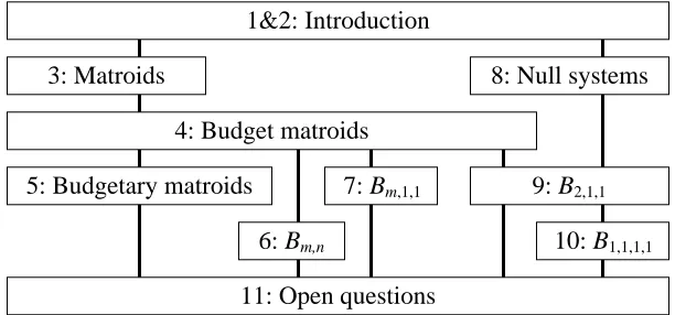
2.6 Testing the 2-dependence of points with a complete quadrangle . 23 2.7 A configuration with 4 auxiliary points that tests 2-dependence . 25 2.8 A configuration with 8 auxiliary points that tests 2-dependence . 26 2.9 The dependencies between the chapters in this monograph . . . 31

3.1 A complete quadrangle with its three diagonal points . . . 35

4.1 A Pappus configuration . . . 39

4.2 A complete quadrilateral, once again . . . 40

4.3 A Pappus configuration with six-fold symmetry . . . 42

5.1 A representation of a certain matroid of rank 4 . . . 66

6.1 Constructing a representation of the matroid B2,2 . . . 77

9.1 Analyzing the P-last construction . . . 114

9.2 A representation of the matroid B2,1,1 . . . 115

9.3 A matroid in the Brazilian jungle. . . 116

9.4 A grid in 3-space . . . 119

(12)

(13)

Preface

0.1 The central question

For work in computer-aided geometric design, as for countless other purposes, we must understand the structure of the univariate polynomials. In particular, we must be able to test for linear dependence. If we know the n+1 coefficients of each of

n+1 polynomials of degree n, we can test for dependence simply by computing an(n + 1)-by-(n + 1)determinant. But there are times — such as when using polar forms [43] to study splines — when what we know about each polynomial is its n roots, rather than its n +1 coefficients. At such times, we can compute the coefficients from the roots, up to an irrelevant scale factor, and then proceed as before. For example, in the quadratic case, the three nonzero polynomials

f1(X)=r1(X−a1)(X −b1)=r1(X2−(a1+b1)X +a1b1)

f2(X)=r2(X−a2)(X −b2)=r2(X2−(a2+b2)X +a2b2)

f3(X)=r3(X−a3)(X −b3)=r3(X2−(a3+b3)X +a3b3) are linearly dependent just when the 3-by-3 determinant

1 a1+b1 a1b1 1 a2+b2 a2b2 1 a3+b3 a3b3

is zero, the numbers(ri)being the irrelevant scale factors. In the cubic case, the

four nonzero polynomials

g1(X)=r1(X −a1)(X −b1)(X −c1)

g2(X)=r2(X −a2)(X −b2)(X −c2)

g3(X)=r3(X −a3)(X −b3)(X −c3)

g4(X)=r4(X −a4)(X −b4)(X −c4) are linearly dependent just when

1 a1+b1+c1 a1b1+a1c1+b1c1 a1b1c1 1 a2+b2+c2 a2b2+a2c2+b2c2 a2b2c2 1 a3+b3+c3 a3b3+a3c3+b3c3 a3b3c3 1 a4+b4+c4 a4b4+a4c4+b4c4 a4b4c4

=0.

(14)

xii PREFACE

P

Q

R

m S

A1

B1

A2

B2 A3

[image:14.612.147.495.88.236.2]

B3

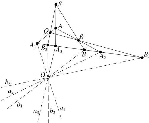
Figure 0.1: A complete quadrangle with vertices(P,Q,R,S)and the quadrangu-lar set{Ai,Bi} i∈[1..3]formed by stabbing that quadrangle with the line m.

In the quadratic case, projective geometry provides an elegant alternative test. Given four points(P,Q,R,S) in the plane with no three collinear, as shown in Figure 0.1, the six lines that join those four points in pairs form an instance of the configuration called the complete quadrangle. The line PQ is called

oppo-site to the line RS, and similarly for the pairs{PR,Q S} and{PS,Q R}. Three pairs of points along a line m are said to form a quadrangular set when they are the intersections of m with the three pairs of opposite lines of some instance of the complete quadrangle. For example, in Figure 0.1, the three pairs {A1,B1}, {A2,B2}, and {A3,B3} form a quadrangular set. Once we fix a coordinate sys-tem for the line m, any pair of points{A,B} on m gives rise to a pair of coordi-nates{a,b}, and those coordinates, in turn, are the roots of a quadratic polynomial

f(X) = r(X −a)(X −b)that is uniquely determined, up to the irrelevant scale factor r. It is a classical result that, given three pairs of points on m, the three poly-nomials so determined are linearly dependent just when the three pairs of points form a quadrangular set.

Here is the central question that sparked this research: Is there a projective con-figuration that provides an analogous geometric test for the linear dependence of four cubic polynomials? Since that configuration would be a cubic analog of the complete quadrilateral, we shall call it the complete cubangle. (Don’t worry: We use that horrid name only in this preface.) Does the complete cubangle exist?

(15)

0.2. A DUALITY WARNING xiii

four triples of planes of some instance of the complete cubangle. Once we fix a coordinate system for the line m, any triple of points{A,B,C} on m determines a triple of coordinates{a,b,c}and hence determines a cubic polynomial g(X)= r(X −a)(X−b)(X−c)uniquely, up to the scale factor r. The analogy requires that, given four triples of points on m, the four cubic polynomials so determined are linearly dependent just when the four triples of points form a cubangular set.

Ta-da! The complete cubangle does exist — that is, there is a configuration that fulfills this analogy. An instance of the complete cubangle consists of twelve planes, two lines, and thirteen points in 3-space, constrained by various incidences. And that’s not all! The complete cubangle is just one member of a large fam-ily of configurations, some familiar and some novel, which we can define using the notion of a budget partition. The complete cubangle is associated with the budget partition(2,1,1), while other budget partitions give rise to other configurations. Defining these configurations and studying their properties involves an intriguing combination of old-fashioned geometry and modern combinatorics. From geom-etry, we use projective frames, projective transformations, and null systems; from combinatorics, we use matroids, minors, and representations.

0.2 A duality warning

One beautiful aspect of projective geometry is the principle of duality, which lets us interchange the concepts ‘point’ and ‘hyperplane’, provided that we also inter-change the concepts ‘lies on’ and ‘passes through’. The complete cubangle con-sists of four triples of planes in 3-space, constrained by their incidences with two lines and thirteen points. The dual configuration consists of four triples of points in 3-space, constrained by their incidences with two lines and thirteen planes. As we discuss in Section 2.6, it turns out to be more convenient to focus on the dual configuration. That is why Chapter 1 begins by discussing, not the complete quad-rangle, but its dual, which is called the complete quadrilateral.

0.3 The accompanying videotape

(16)

xiv PREFACE

0.4 Acknowledgments

First, I want to thank Jorge Stolfi for lots of help and lots of ideas. Jorge’s searching questions sparked Sections 5.4, 10.3, and 10.4. He gets the bulk of the credit for Section 4.5 and every ounce of the credit for Section 11.4. On top of all that, he drew the cartoon.

I thank and praise my colleagues Allan Heydon and Greg Nelson for writing Juno-2 [18], the constraint-based drawing editor that I used to produce both the figures in this monograph and the 2D portions of the videotape. In a similar vein, I thank and praise Marc A. Najork and Marc H. Brown for writing the Anim3D library [35] and the Obliq-3D system [36], which I used for the 3D portions of the videotape.

I am grateful also to J¨urgen Richter-Gebert for his insightful comments on a draft of this monograph.

Finally, my thanks go to Jim Saxe for contributing his formidable expertise and intuition to our joint investigation of this pretty mathematics. While we explored the mathematics jointly, the words and pictures in the monograph and videotape are mine, so the blunders that no doubt remain in them are all my fault.

Lyle Ramshaw

(17)

Chapter 1 Preview

The preface describes the central question out of which this monograph grew. This preview summarizes the results of the monograph, to give you some sense, in ad-vance, of where we are heading. It’s not going to be until Chapter 2 that we finally get around to introducing the material in depth.

1.1 Prerequisites

In order to understand this monograph, you have to know something about projec-tive geometry and something about matroids.

Projective geometry is a standard topic. Good places to start are the books by Coxeter [8] and by Samuel [48]. A valuable supplement, particularly as re-gards computations using homogeneous coordinates and Pl¨ucker coordinates, is Stolfi’s book [50] — although Stolfi discusses oriented projective geometry, which we don’t need, because our matroids are not oriented [5].

As for matroids, the books by Oxley [37] and by Welsh [52] are fine sources. Because matroid theory isn’t yet as standard a topic as projective geometry, we take the time, in Chapter 3, to review the definition of a matroid and some of the elementary properties of matroids.

1.2 Configurations and dependent polynomials

The complete quadrilateral, an instance of which is shown in Figure 2.2 on page 7, is a projective configuration with six points and four lines. It is a standard re-sult that the complete quadrilateral characterizes the dependence of three quadratic polynomials. As for what it means to ‘characterize dependence’, two theorems are involved, which we shall call the Projection Theorem and the Witness Theorem. (Warning: Those names are not standard, as discussed in Section 2.5.)

Given any instance of the complete quadrilateral and given any point in the plane O, we can project the six vertices of the quadrilateral from O to get six lines

(18)

2 CHAPTER 1. PREVIEW

through O. The Projection Theorem says that the three univariate, quadratic poly-nomials that have the slopes of those six lines as their roots are always linearly dependent.

Conversely, suppose that we take any six numbers that are the roots of three linearly dependent quadratics, we take any point O in the plane, and we draw the six lines through O with those slopes. The Witness Theorem says that there exists an instance of the complete quadrilateral whose six vertices lie on those six lines, and which hence witnesses to the linear dependence of those three quadratics. Fur-thermore, there is a natural sense in which the witnessing quadrilateral is unique: Any two witnessing quadrilaterals are related by a projective transformation of the plane that fixes the point O and fixes every line through O.

Here is the first half of the good news in a nutshell:

There is a projective configuration B2,1,1in 3-space — consisting of twelve points, two lines, and thirteen planes — that characterizes the dependence of four cubic polynomials in the same way that the complete quadrilateral in the plane characterizes the dependence of three quadratic polynomials.

In particular, there are cubic analogs of the Projection Theorem and the Witness Theorem that hold for the configuration B2,1,1. Note that we project an instance of the configuration B2,1,1from a line o in 3-space, rather than from a point O in the plane. The twelve vertices of the configuration determine twelve planes through the line o, the slopes of which are the roots of four cubic polynomials that are al-ways linearly dependent.

1.3 The budget matroids

A matroid is an algebraic structure that describes the pattern of incidences — the collinearities, coplanarities, and the like — that are required of the points in a pro-jective configuration (it being understood that every incidence that is not required is forbidden). So, roughly speaking, ‘matroid’ is the modern term for ‘projective configuration’. If the matroid M describes the incidences of some configuration

C, then a representation of M is the same thing as an instance of C; and a matroid

is representable when it has representations.

The incidences of the complete quadrilateral are described by a matroid that we shall call B2,1. The justification for that name comes from the other half of the good news:

For each partition b =b1+· · ·+bkof an integer b into at least two

positive parts, we can define an associated matroid, which we shall call the budget matroid Bb1,...,bk. A surprising number of these budget

(19)

1.3. THE BUDGET MATROIDS 3

is described by the matroid B2,1, while the configuration in 3-space proclaimed above is described by the matroid B2,1,1.

In more detail, let b = b1 + · · · +bk be some partition of an integer b into

at least two positive parts. The budget matroid Bb1,...,bk has rank b and has, as its

ground set, a matrix _

   

E11 E12 . . . E1k

E21 E22 . . . E2k

... ... ... ...

Eb1 Eb2 . . . Ebk

    

consisting of bk points. The rules for independence in the matroid Bb1,...,bk force

the b points in the jth_{column to lie in a common flat subspace of dimension b}

j, for

each j in [1. .k]. Also, for each possible way of choosing b points so that precisely

one is chosen from each row and so that, for each j , precisely bj are chosen from

the jth_{column, the b points so chosen must lie in a common hyperplane. Here are} geometric descriptions of the representations of the budget matroids of rank b =3:

• B2,1: the six vertices of a complete quadrilateral in the plane.

• B1,1,1: the nine points of a Pappus configuration in the plane, as shown in Figure 4.1 on page 39.

Here are similar descriptions for rank b=4:

• B3,1: the four vertices of a tetrahedron in 3-space, together with the four points where a line cuts its four faces.

• B2,2: the eight vertices of a M¨obius pair of tetrahedra — that is, two tetrahe-dra with the vertices of each lying on the faces of the other.

• B2,1,1: twelve points in 3-space, four on a plane, four each on each of two lines, and with 12 other coplanarities in a certain pattern. This is the config-uration that characterizes the dependence of four cubic polynomials. • B1,1,1,1: sixteen points in 3-space, four each on each of four lines and with

24 coplanarities in a certain pattern.

We prove two general results about the representability of the budget matroids: Every budget matroid Bm,n with two parts is representable over the rationals, as is

every matroid Bm,1,1with three parts, two of which are ones. The latter result can be interpreted as generalizing Pappus’s Theorem from the plane to(m+1)-space. In the particular case m = 2, the latter result gives us one construction for repre-sentations of the budget matroid B2,1,1.

(20)

4 CHAPTER 1. PREVIEW

the choices in a different order. This second construction exploits the properties of

null systems, the little-known cousins of the well-known polar systems that are

as-sociated with quadric hypersurfaces. We use the same null-system machinery also to construct representations of B1,1,1,1, the most complicated of the budget matroids of rank 4.

1.4 The bad news about the quartic case

(21)

Chapter 2 Introduction

2.1 The quadratic case

The quadratic polynomial X2 −(u +v)X +uv has the pair of scalars{u, v} as its roots.1 _{Let us say that three pairs of scalars}{_u

1, v1},{u2, v2},{u3, v3} form a 2-dependent block when the three quadratic polynomials with those pairs as their roots are linearly dependent, that is, when the determinant

1 u1+v1 u1v1 1 u2+v2 u2v2 1 u3+v3 u3v3

is zero. Note that the order of the two scalars{ui, vi}in a pair doesn’t affect the

2-dependency of the block, nor does the order of the three pairs.

By the way, you can think of the scalars that we deal with, such as ui andvi,

as either rational numbers, real numbers, or complex numbers, as suits your fancy. More formally, we fix some field of scalars in which to carry out our numeric com-putations and over which to build our projective spaces. Unless otherwise stated, we require only that the scalar field have characteristic zero — that property being all that we need for the bulk of our arguments. Of course, when we want to illus-trate a geometric construction with a picture, it is simplest to assume that the field of scalars is the real numbers.

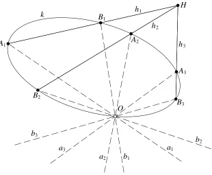
The algebraic condition of 2-dependence corresponds to a simple geometric condition involving a conic curve in the plane. Let O be a point in the plane, and let{a1,b1},{a2,b2},{a3,b3} be three pairs of lines through O, as shown (over the real numbers) in Figure 2.1. Each of the lines has a scalar slope, and when those slopes form a 2-dependent block of scalars, we shall refer to the block of lines itself as 2-dependent. To test a block of lines for 2-dependence, let k be any

1_{The expression}_{_u_{, v}_}_{denotes a pair of roots, even when u}₌_v_{; that is, the curly braces here}

indicate a suite [45] or multiset or bag, rather than a set. But please ignore all degenerate cases, as much as you can, until Section 2.4.

(22)

6 CHAPTER 2. INTRODUCTION

O

a1

b1

a2

b2

a3

b3

H h1

h2

h3

A1

B1

A2

B2

A3

B3

[image:22.612.161.471.88.343.2]

k

Figure 2.1: A 2-block of lines, all passing through a common point O, whose 2-dependence is demonstrated by the concurrence of three chords of a conic curve

k that also passes through the point O.

conic passing through the point O. Any line through O intersects the conic k at O itself and at one other point. Let hi := AiBi be the chord of the conic k joining the

residual intersections of the lines ai and bi, for i in [1. .3]. It is straightforward

to check (see Exercise 2.1-4) that the block of lines{a1,b1},{a2,b2},{a3,b3} is 2-dependent just when the three chords h1, h2, and h3of the conic k are concurrent — that is, pass through a common point H .

It is a fascinating result of classical projective geometry that 2-dependence can be characterized in an even simpler way, at the cost of some loss of symmetry. The four auxiliary lines a, q, r, and s in Figure 2.2 intersect at the six points

A1 :=a∩q B1 :=r ∩s

A2 :=a∩r B2 :=q∩s

A3 :=a∩s B3 :=q∩r.

These six points and four lines are called a complete quadrilateral. More precisely, they are an instance of the classical configuration called the complete

quadrilat-eral; that is, the name of the pattern is used also for instances of that pattern. For i

in [1. .3], the two points Ai and Bi are called opposite, since they lie on no

(23)

2.1. THE QUADRATIC CASE 7

O

a1

b1

a2

b2

a3

b3

A1

B1

A2

B2

A3

B3

a q

[image:23.612.112.483.87.292.2]

r s

Figure 2.2: The same 2-block of lines as in the previous figure, but with their 2-dependence demonstrated, this time, by a witnessing complete quadrilateral.

an ordered block, that is, as an unordered triple of ordered pairs. So, for each pair of opposite vertices(Ai,Bi), we know which of them is the A-point and which is

the B-point. The A-points of the three pairs are collinear, along the auxiliary line

a; and the A-point of any pair is collinear with the B-points of the other two pairs,

along some other of the auxiliary lines.

Given an ordered block of points that form a complete quadrilateral and given any point O in the plane, we can project the three pairs of points from the point O — which is called, in this context, the center of the projection — to get an ordered block of lines{(a1,b1), (a2,b2), (a3,b3)}through O. It turns out that this block of lines is always 2-dependent. We call this result the Projection Theorem, and we discuss its proof in Section 2.5.

Conversely, given any ordered block of lines through a common point O that is 2-dependent, there exists a complete quadrilateral each of whose six vertices lies on the appropriate line and which hence witnesses to the 2-dependence. Of course, this witnessing quadrilateral is not unique. It is clear that any projective transfor-mation of the plane that fixes the point O and fixes every line through O carries any witnessing quadrilateral to another quadrilateral that is also a witness. But the witnessing quadrilateral is unique up to such transformations; that is, any witness-ing quadrilateral can be mapped to any other by a projective transformation of the plane that fixes both the point O and every line through O. We call this converse result the Witness Theorem, and we discuss its proof also in Section 2.5.

(24)

O b3

a3

b1

a1

a2

b2

B3

A3

B1

A1

A2

B2

A3′

B1′

B2′

B3′

A1′

[image:24.612.147.485.89.289.2]

A2′

Figure 2.3: An unordered block of lines and two complete quadrilaterals that wit-ness to the 2-dependence of that block, but under different orderings thereof.

in Figure 2.2. (Coxeter [9] relates this broken symmetry to the axioms for projec-tive geometry.) Suppose that we arbitrarily select the line a1from the pair{a1,b1} and the line a2from the pair{a2,b2}. Even after we have made those selections, the two lines a3and b3 in Figure 2.1 play completely symmetric roles. But not so in Figure 2.2: The point A3 on the line a3is collinear with A1 and A2, while the point B3is not. Thus, once we have ordered two of the three pairs in Figure 2.2, the third pair acquires an order as well. We can swap any even number of pairs without changing anything. If we swap an odd number of pairs, we still don’t af-fect the 2-dependency of the block of slopes; but we do change the structure of the witnessing quadrilaterals.

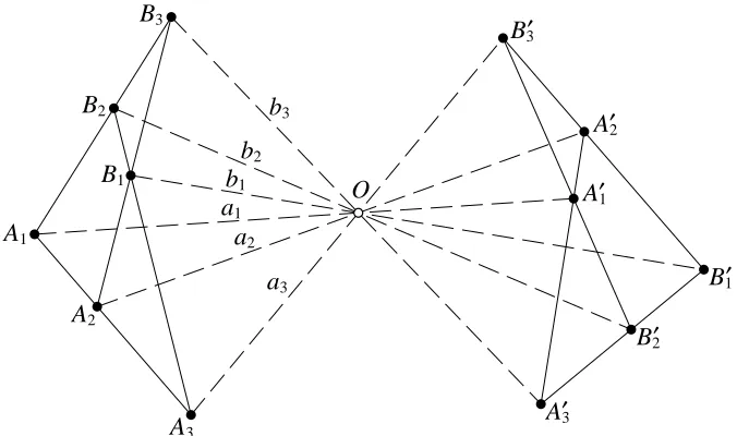
Something must be done about this broken symmetry, lest the uniqueness claim in the Witness Theorem fail. Figure 2.3 shows a 2-dependent, unordered block of lines{a1,b1},{a2,b2},{a3,b3} through a point O. It also shows two complete quadrilaterals, one on the left and one on the right. The one on the left witnesses to the 2-dependence of the obvious ordered block{(a1,b1), (a2,b2), (a3,b3)}, while the one on the right witnesses, instead, to the 2-dependence of the ordered block {(a1,b1), (a2,b2), (b3,a3)}, in which the single pair (a3,b3) has been swapped. Note that no projective transformation that fixes O and every line through O can possibly map the left quadrilateral to the right one. Any such transformation would have to map A1 7→ A0₁, A2 7→ A0₂, and A3 7→ B₃0; but the points A1, A2, and A3 are collinear, while the points A0₁, A0₂, and B₃0 are not.

(25)

de-2.1. THE QUADRATIC CASE 9

fined a complete quadrilateral to be an ordered block of points. When a complete quadrilateral witnesses to the 2-dependence of a block of lines or slopes, we treat that block also as ordered.

Exercise 2.1-1 Count the degrees of freedom in the Witness Theorem, so as to verify that its claims of existence and uniqueness are at least plausible.

[Answer: Fix a center point O in the plane, and consider 2-dependent blocks of lines through O and the complete quadrilaterals that witness to their 2-dependence. There are five degrees of freedom in choosing such a 2-dependent block: six scalar slopes, related by one equation. There are eight degrees of freedom in choosing a complete quadrilateral: two in each of its four lines. Thus, for each 2-dependent block of lines through O, there must be a 3-parameter family of quadrilaterals that witness to the 2-dependence of that block. The Witness Theorem says that any such witness can be mapped to any other by a projective transformation of the plane that fixes both the point O and every line through O. There are eight degrees of freedom in an arbitrary projective transformation of the plane — any four points, no three collinear, to any other four such points. Of those eight, it takes four to fix two chosen lines through O, which fixes the point O as well. It takes one more to fix all of the remaining lines through O. The three degrees of freedom that are left are just enough to map any witness to any other.]

Exercise 2.1-2 Given five lines a1, a2, b1, b2, and b3 through a point O in the plane, use a complete quadrilateral to construct the unique sixth line a3 through

O that makes the ordered block{(ai,bi)}i∈[1..3]of lines 2-dependent.

[Answer: Choose Bi arbitrarily on bi, for i in [1. .3], thus using up the three

degrees of freedom that are involved in choosing a witness. Then construct A1 :=

a1∩ B2B3, A2 :=a2∩B1B3, A3 := A1A2 ∩B1B2, and a3 := O A3.]

Exercise 2.1-3 In this exercise, the field of scalars must be ordered; for simplicity, let’s use the real numbers. A pair{ui, vi}of real numbers is said to separate another

pair{uj, vj}when the product(uj−ui)(uj−vi)(vj−ui)(vj−vi)is negative. Let

{u1, v1},{u2, v2},{u3, v3} be six distinct, real numbers that form a 2-dependent block. Show that either each pair separates both of the other pairs or else no two pairs separate each other.

[Hint: In Figure 2.1, does the point H lie inside or outside of the conic k? Al-ternatively, in Figure 2.2, the auxiliary lines a, q, r, and s divide the real projective plane into seven regions: four triangles (two of which are finite) and three quadri-laterals (one of which is finite). Does the center point O lie in a triangle or in a quadrilateral?]

(26)

[Hint: We can choose our coordinate system on the projective plane so that the point O is the origin and the conic k is the standard parabola Y = X2. The line through O with slope t then cuts the conic k at the point(X,Y)=(t,t2₎_{. Letting} the scalars ui andvi, for i in [1. .3], denote the slopes of the lines ai and bi, it

follows that the chord hi is the line with the equation Y −(ui+vi)X+uivi =0.

Deduce from this that the three chords are concurrent just when the six slopes are 2-dependent.]

2.2 Generalizing to n

>

2

To what extent does this theory generalize to degrees n greater than 2?

Let’s define an unordered n-block — of scalars, points, lines, planes, or what-ever — to be an unordered(n+1)-tuple of unordered n-tuples. An ordered n-block, on the other hand, is an unordered(n+1)-tuple of ordered n-tuples.

It is easy to define n-dependence algebraically, for any n. We say that an un-ordered n-block of scalars{ui j}j∈[1..n] i∈[0..n] is n-dependent when the n+1

poly-nomials

(X −u01)(X−u02)· · ·(X −u0n)

(X −u11)(X−u12)· · ·(X −u1n)

... ... ... ...

(X−un1)(X −un2)· · ·(X −unn)

of degree n that have those n-tuples as their roots are linearly dependent. We can test this by forming an (n + 1)-by-(n +1)matrix whose ith _{row consists of the} elementary symmetric polynomials in the entries ui1through uinof the ithtuple and

checking whether the determinant vanishes. For example, the unordered 3-block of scalars{ui, vi, wi} _i_∈_[0_.._3] is 3-dependent just when

1 u0+v0+w0 u0v0+u0w0+v0w0 u0v0w0 1 u1+v1+w1 u1v1+u1w1+v1w1 u1v1w1 1 u2+v2+w2 u2v2+u2w2+v2w2 u2v2w2 1 u3+v3+w3 u3v3+u3w3+v3w3 u3v3w3

=0.

Before we can test for n-dependence geometrically, we first have to decide how to encode scalars geometrically; we’re going to use the slopes of the hyperplanes in a pencil of hyperplanes in n-space. Recall that a pencil consists of all of the hyper-planes that pass through a fixed flat subspace of dimension n−2, which is called the

center of the pencil. So the hyperplanes in a pencil form a one-parameter family,

with slope as the parameter. For example, when n=2, we test the 2-dependence of a 2-block of lines in the plane, all passing through a common center point. When

(27)

2.2. GENERALIZING TO n >2 11

common pencil, is n-dependent just when the slopes of those hyperplanes form an

n-dependent block of scalars. As we discuss in Section 2.5, it doesn’t matter what

scale we use to measure slopes.

It is easy to test for n-dependence geometrically using a curve. The role that is played by a conic when n =2 is played, in the general case, by a rational normal curve of degree n in projective n-space [15, 47]. For example, when n = 3, the relevant curve is a twisted cubic in 3-space — one example of which is the curve given parametrically by t 7→ (t,t2,_t3)_{. Let} {αi, βi, γi}

i∈[0..3] be an unordered 3-block of planes, all through a common line o. Choose a twisted cubic k that in-tersects the center line o at two points — that is, so that o is a chord of k. Any plane through o intersects k at three points: the two points where o intersects k and one residual intersection. Given a triple of planes{α, β, γ} through o, let A,

B, and C denote the residual intersections of those three planes with the twisted

cubic k, and letηbe the planeη:= ABC. The block of planes{αi, βi, γi} _i_∈_[0_.._3]

is 3-dependent just when the four planesηi := AiBiCi determined by the residual

intersections are concurrent.

But it isn’t at all clear how to take the test for 2-dependence that is based on complete quadrilaterals and to generalize that into a test for n-dependence. Is there a projective configuration in n-space that characterizes n-dependence in the same way that the complete quadrilateral in the plane characterizes 2-dependence? For example, when n =3, is there some pattern of collinearities and coplanarities that we can impose on twelve points in 3-space so that, for any twelve points with those incidences and for any additional line o, projecting the twelve points from o will re-sult in twelve planes whose slopes are 3-dependent? Conversely, given any twelve planes whose slopes are 3-dependent, does there always exist an instance of this hypothetical configuration that witnesses to that 3-dependence? The main goal of this monograph is to study such a configuration — one for which cubic analogs of both the Projection and Witness Theorems hold.

Recall that using a complete quadrilateral to test for 2-dependence breaks some of the inherent symmetry, which is why we introduced ordered 2-blocks. Since the symmetry gets broken already when n = 2, it seems likely that it will be broken also when n > 2. Hence, just as we defined an instance of the complete quadri-lateral to be an ordered 2-block of points in the plane, we expect an instance of its cubic analog to be an ordered 3-block of points in 3-space. And we expect the Witness Theorem in the cubic case to talk about such an instance as witnessing to the 3-dependence of an ordered 3-block of planes, all in a common pencil.

Exercise 2.2-1 When does the 1-block{u0},{u1} formed by two singletons of scalars have the property of 1-dependence?

[Answer: When u0 =u1.]

(28)

12 CHAPTER 2. INTRODUCTION matrix _                

u01 u02 . . . u0n

u11 u12 . . . u1n

u21 u22 . . . u2n

... ... ... ...

un1 un2 . . . unn

                 .

Show that there is typically a unique value for the final scalar that makes the rows of the resulting matrix form an n-dependent block. What can happen in atypical cases?

[Hint: Consider the cases

      

−1 −1

1 1 0 u        and        0 0 0 1 0 u       .

Keep in mind, in the former case, that not all lines have finite slope.]

Exercise 2.2-3 Justify the geometric test for 3-dependence based on a twisted cu-bic curve, hence generalizing Exercise 2.1-4 to the cucu-bic case.

[Hint: We can choose our coordinate system on projective 3-space so that the center line o is the Z -axis and the twisted cubic k is given parametrically by the function t 7→ (t,t2,_t3)_{. Note that the line o intersects the cubic k at the origin,} where t = 0, and also at the point at infinity on the Z -axis, where t = ∞. The equation of a plane through o has the form Y =t X, and we can treat the t in this

equation as the slope of the plane. The plane Y = t X with slope t then has the

point(t,t2,t3)as its residual intersection with the cubic k. Letting ui,vi, andwi,

for i in [0. .3], denote the slopes of the planesαi,βi, andγi, show that the plane

ηi determined by the three residual intersections has the equation

Z −(ui +vi +wi)Y +(uivi +uiwi +viwi)X −uiviwi =0.

Deduce from this that the four planes(ηi)are concurrent just when the four triples of slopes are 3-dependent.]

2.3 Configurations versus constructions

Our goal is to find a configuration in 3-space that characterizes 3-dependence in the same way that the complete quadrilateral in the plane characterizes 2-dependence. To clarify what that means, we should discuss several things that could be our goal, but aren’t. For one thing, it is not our goal simply to devise a geometric construc-tion that tests for n-dependence.

(29)

2.3. CONFIGURATIONS VERSUS CONSTRUCTIONS 13

a complete quadrilateral, as in Exercise 2.1-2, and we then check to see if the sixth comes out properly. The resulting complete quadrilateral witnesses either to the 2-dependence of the six slopes or to their lack of 2-dependence. The case n =3 is similar. Given four triples of planes through a common line, we can use any eleven of them to construct an instance of the configuration B2,1,1that witnesses either to the 3-dependence of the twelve slopes or to their lack of 3-dependence.

But there are lots of constructions that test for n-dependence; devising such a construction is too easy to be a worthwhile goal. When n = 2, the construction based on complete quadrilaterals is probably the simplest, and it is hence featured in textbooks.2 _{But we make no claim that, when n} =_{3, the construction based on} the configuration B2,1,1is the simplest or the best. It may be in the running for the shortest, but it involves lots of degenerate cases that would require special treat-ment, as discussed in Section 9.6. Our central interest is the configuration itself, not the associated construction.

Just how easy is it to test for n-dependence with a construction? The simplest constructions in the plane are those that can be carried out using only a straight-edge. There is no standard name for the geometric tool in n-space that is analogous to a straightedge, but it is clear what it should do; we shall call it a flat-side. (To carry out a geometric construction in the plane, you look through your pile of scrap lumber for a strip with a straight edge; to carry out a construction in 3-space, you look instead for a board with a flat side.) In the plane, a straightedge lets us mark a line`in such a way that the unique point common to`and to a second, marked line is distinguished as doubly marked. In 3-space, a flat-side lets us mark a plane

π in such a way that the line common toπand to a second marked plane is distin-guished as doubly marked, while the point common toπ and to two other marked planes is distinguished as triply marked. A flat-side in n-space lets us mark hyper-planes in an analogous way.

It is well known that addition and multiplication can be carried out geometri-cally, using a straightedge in the plane. Hence, we can test n-dependence geomet-rically for any n with just a straightedge, by mimicking the algebraic definition: Construct the determinant of the(n+1)-by-(n+1)matrix — that is, construct a segment whose length represents that determinant — and test it for zero. We can shorten the construction quite a bit by moving from the plane to n-space. Instead of constructing the determinant itself, we set up a coordinate system in n-space, we construct the n+1 points whose homogeneous coordinates are given by the rows of the matrix, and we then use a flat-side to test whether those n+1 row-points lie on a common hyperplane.

We can devise another construction that tests for n-dependence by exploiting a rational normal curve of degree n. Of course, with a flat-side as our only tool, we can’t draw the rational normal curve itself. But there is no need to do so. Using

2_{Actually, it is the dual construction, based on complete quadrangles, that is generally featured}

(30)

only a flat-side, we can choose such a curve and we can construct the residual in-tersections of the n(n+1)given hyperplanes with that chosen curve, as discussed in the following exercises; and that is enough.

Exercise 2.3-1 Implement the test for 2-dependence based on a conic curve — the one shown in Figure 2.1 — using only a straightedge.

[Hint: Choose four points O0, P1, P2, and P3so that no three of the five points

(O,O0,P1,P2,P3)are collinear. There is a unique projective correspondence be-tween the pencil of lines through O and the pencil through O0 in which the line

pi := OPi corresponds to the line pi0 :=O0Pi, for i in [1. .3]. The intersections of

corresponding lines in those two pencils trace out a conic k. Let a₁0 be the line in the O0pencil whose cross ratio with respect to(p0₁,p₂0,p0₃)is the same as the cross ratio of a1with respect to(p1,p2,p3). The residual intersection A1of the line a1 with the conic k is the point A1 :=a1∩a10.]

Exercise 2.3-2 Using only a flat-side, implement the test for 3-dependence based on a twisted cubic curve.

[Hint: Given twelve planes through the line o, choose two lines o0and o00 that are skew to each other and to o, and choose three points P1, P2, and P3in general position. There are unique projective correspondences between the three pencils of planes with axes o, o0, and o00 in which the planes πi := Span(o,Pi),π_i0 :=

Span(o0,Pi), andπi00 :=Span(o00,Pi)correspond, for i in [1. .3]. The intersections π∩π0_∩_π00_{of corresponding planes in the three pencils trace out a twisted cubic}

through P1, P2, and P3 of which the lines o, o0, and o00 are chords.]

2.4 Dealing with degeneracies

The claims made in the previous sections are true generically, but some of them may fail in degenerate cases, where a case is degenerate when some polynomial relation among the input parameters that usually doesn’t hold happens to hold. For example, we treated slopes above as finite scalars, and they usually are; but there do exist lines with infinite slope. There are fundamentally two ways to deal with a degenerate case: Either we handle it or we outlaw it.

We handle a degenerate case by extending our definitions in some clever way, after which that case is no longer degenerate. For example, there is a standard way to handle the degenerate case of lines with infinite slope. We represent a slope, not as a single scalar u, but as the ratio u↑: u↓of two scalars3u↑ :=1y and u↓:=1x ,

which are called homogeneous coefficients — ‘homogeneous’ because multiplying them both by the same nonzero scalar doesn’t change their ratio. Either of the ho-mogeneous coefficients can be zero, but not both, and the slope of a vertical line is represented by the ratio u↑ : u↓ = 1 : 0. In this way, we can extend the algebraic

(31)

2.4. DEALING WITH DEGENERACIES 15

definition of n-dependence to handle infinities — that is, we can extend it from the affine line to the projective line. In the quadratic case, the polynomial with the two ratios u↑ _{: u}↓_and_v↑ _: _v↓_{as its two roots is}₍_u↓_X ₋_u↑_)(v↓_X ₋_v↑₎_{, and the three}

polynomials

(u↓₁X −u↑₁)(v₁↓X −v₁↑)=u↓₁v₁↓X2−(u↓₁v₁↑+u₁↑v₁↓)X+u↑₁v₁↑

(u↓₂X −u↑₂)(v₂↓X −v₂↑)=u↓₂v₂↓X2−(u↓₂v₂↑+u₂↑v₂↓)X+u↑₂v₂↑

(u↓₃X −u↑₃)(v₃↓X −v₃↑)=u↓₃v₃↓X2−(u↓₃v₃↑+u₃↑v₃↓)X+u↑₃v₃↑

are linearly dependent just when

u↑₁v₁↑ u↑₁v↓₁+u↓₁v₁↑ u↓₁v₁↓ u↑₂v₂↑ u↑₂v↓₂+u↓₂v₂↑ u↓₂v₂↓ u↑₃v₃↑ u↑₃v↓₃+u↓₃v₃↑ u↓₃v₃↓

=

0. (2.4-1)

In forming this determinant, we dropped the minus signs in the middle column, as we have been doing all along; we also swapped the first and third columns, to make the highs come before the lows in each row, as is the case in the ratio u↑: u↓. Projective geometry adroitly handles the many degenerate cases that are asso-ciated with parallelism in a similar way. It extends n-dimensional affine space into

n-dimensional projective space by moving from n affine coordinates(X1, . . . ,Xn)

to n+1 homogeneous coordinates [x0,x1, . . . ,xn], where Xi =xi : x0. Following Stolfi [50], we shall use square brackets to delimit the homogeneous coordinates of a point and angle brackets to delimit the homogeneous coefficients of a hyper-plane. So the hyperplanehc0,c1, . . . ,cnipasses through the point [x0,x1, . . . ,xn]

just when c0x0+c1x1+· · ·+cnxn =0. Dividing through by the weight coordinate

x0of the point converts this equation into c0 +c1X1+ · · · +cnXn = 0, which is

the inhomogeneous equation of that same hyperplane.

If we don’t know how to handle a degenerate case, we can outlaw it. For exam-ple, consider defining 2-dependence using a conic curve, as in Figure 2.1. Some of the degenerate cases that arise are straightforward to handle:

• One of the lines through O, say a1, might be tangent to the conic k — in which case we set A1 := O.

• The two lines in a pair, say a1 and b1, might coincide — in which case the chord h1becomes a tangent.

• Two of the pairs of lines might coincide, say {a1,b1} = {a2,b2} because

a1 = b2 and a2 = b1, causing the two chords h1 and h2 to coincide — in which case the three chords are bound to concur.

(32)

Sometimes, it is simpler to outlaw a degenerate case, even though it could be handled. For example, we want the Projection Theorem to hold; so we must de-fine the notion ‘complete quadrilateral’ in such a way that projecting the six ver-tices of any complete quadrilateral, as in Figure 2.2, gives six lines whose slopes are 2-dependent. We clearly can’t allow all four of the auxiliary lines a, q, r, and

s to coincide and the six points of intersection{(A1,B1), (A2,B2), (A3,B3)} to vary arbitrarily and independently along that common line. But lesser degenera-cies wouldn’t hurt: three of the lines being concurrent, two of them coinciding, even three of them coinciding. Despite this, we shall opt for simplicity — and fol-low the textbooks — by insisting, as part of our definition of a complete quadrilat-eral, that no three of its four lines are concurrent. In a similar way, when defining our cubic analog of the complete quadrilateral, we shall stipulate that every inci-dence that is not required is forbidden.

In the quadratic Projection and Witness Theorems, there are also issues of de-generacy about the location of the complete quadrilateral with respect to the cen-ter point O of the projection. The approach taken in the textbooks is to outlaw any 2-block of lines in which two lines in different pairs coincide. Exercise 2.4-3 below explains why that prohibition suffices to eliminate all of the troublesome degeneracies. Adopting that approach and fixing a center point O leads to the fol-lowing tidy results:

Projection Theorem If none of the four lines of a complete quadrilateral passes through the center point O, then projecting the three pairs of vertices of that quadrilateral from O gives an ordered, 2-dependent block of lines in which no line in any pair coincides with any line in any other pair.

Witness Theorem Conversely, suppose that we are given any ordered, 2-depen-dent block of lines through O in which no line in any pair coincides with any line in any other pair. Then, there exists a complete quadrilateral whose six vertices lie on the appropriate lines and none of whose four lines passes through O. Furthermore, any two such witnessing quadrilaterals are related by a unique projective transformation of the plane that fixes the point O and every line through O.

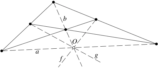
Note that the two lines in a single pair are allowed to coincide. They do so precisely when the center point O lies on a diagonal of the complete quadrilateral, the diagonals of a complete quadrilateral being the three lines that join the opposite pairs of vertices. Indeed, the center point O may lie at the intersection of two of the three diagonals, as shown in Figure 2.4, and this is an important special case. In the pencil of lines through a point O, a line f is called the harmonic conjugate [10] of a line g with respect to two distinct lines a and b just when the block of lines

{a,a},{b,b},{f,g} is 2-dependent.

(33)

2.4. DEALING WITH DEGENERACIES 17

O a

b

[image:33.612.161.430.92.208.2]

f g

Figure 2.4: Two pairs of lines{a,b} and{f,g}through a common point O that form a harmonic set; that is, each line of each pair is the harmonic conjugate of its mate with respect to the two lines of the other pair.

wider variety of troubles. Note that it is easy to recognize the 2-dependent blocks that might cause trouble, because, as shown in Exercise 2.4-3, they all have at least two entries that are equal. In contrast, a 3-dependent block can cause trouble even when all twelve of its entries are distinct — see Exercise 2.4-4 for an example. We discuss some of the degenerate cases of the cubic Projection and Witness The-orems in Section 9.6, and we speculate on how they might be handled. But, in proving those theorems, we take the coward’s way out by restricting ourselves to the generic case — those instances in which no troublesome degeneracies arise.

Exercise 2.4-2 Convince yourself that an ordered block{(Ai,Bi)}i∈[1..3]of points in some projective space forms a complete quadrilateral in the strict sense — that is, where we forbid every incidence that is not required — just when

• none of the 6₂=15 pairs of points coincides;

• every one of the 6₄ =15 quadruples of points is coplanar; and

• among the 6₃ = 20 triples of points, just the following four are collinear: {A1,A2,A3},{A1,B2,B3},{B1,A2,B3}, and{B1,B2,A3}— those four cor-responding to the four auxiliary lines a, q, r, and s in Figure 2.2.

Exercise 2.4-3 Suppose that _

     

u v

w x

y z

      

is a 2-dependent block of scalars; so the determinant

1:=

1 u+v uv

1 w+x wx

1 y+z yz

(34)

is zero. If either entry in some pair equals either entry in some other pair, show that a second equality also holds, and show that any entry not involved in either equal-ity can be varied freely, while holding all other entries fixed, without destroying the 2-dependence. Conversely, if there exists any entry that can be varied freely without destroying the 2-dependence, show that some entry in some pair equals some entry in some other pair.

[Hint: For the first part, we can assume without loss of generality that u =w, in which case the determinant1factors as1=(x−v)(y−u)(z−u). Since1=0, some other equality must hold, and any entry not involved in either equality can be varied freely.

For the second part, solving the equation1=0 for z yields

z= uvw+uvx −uvy+wx y−uwx −vwx x y+wy−wx +uv−vy−uy .

Suppose that z can be varied freely, which means that both the numerator N and denominator D of that fraction are zero. It then follows that

(w+x −u−v)N −(wx−uv)D= (w−u)(w−v)(x −u)(x−v)=0,

so some entry in the first pair equals some entry in the second pair.]

Exercise 2.4-4 Note that, in the 2-dependent block

       0 1 0 1 0 1       ,

we can vary both of the elements in any single row freely and independently, with-out destroying the 2-dependence. Show that the analogous property holds of the following 3-dependent block, even though all of its entries are distinct:

          

1 9 −10

−1 −9 10

5 6 −11

−5 −6 11

          

That is, show that the 4-by-4 matrix formed from the coefficients of the cubic poly-nomials with those triples of roots not only has determinant zero, but actually has rank only 2.

2.5 Proving the quadratic case

(35)

2.5. PROVING THE QUADRATIC CASE 19

The Projection and Witness Theorems do not appear, as such, in standard texts on projective geometry, for the excellent reason that 2-dependence is an algebraic notion, not a geometric one. But those books do provide pieces which we can as-semble into a proof. Coxeter [12] shows that the six lines{ai,bi} i∈[1..3]through a point O are the projections of the six vertices of a complete quadrilateral just when there exists an involution — that is, a self-inverse projectivity — of the pencil of lines through O that swaps ai with bi, for each i. Maxwell [33] shows that such an

involution exists precisely when the three chords of the conic in Figure 2.1, that is, the lines hi := AiBifor i in [1. .3], are concurrent. And we already showed, in

Ex-ercise 2.1-4, that the three chords(hi)are concurrent precisely when the six slopes

have the algebraic property of 2-dependence. That chain of reasoning suffices to prove the Projection Theorem and the existence half of the Witness Theorem.

That assembled proof has a couple of unfortunate aspects: It doesn’t establish the uniqueness half of the Witness Theorem, and it relies on the concept of an in-volution — a concept that would be somewhat clumsy to generalize to the cubic case. Fortunately, it isn’t hard to prove the Projection Theorem and both halves of the Witness Theorem directly. Let’s do that, since proving the quadratic case directly will help to prepare us for proving the cubic case, in Chapter 9.

We begin with an overdue lemma about n-dependence. When we are testing an n-block of hyperplanes for n-dependence, it doesn’t matter what scale we use to measure the slopes of the hyperplanes in that pencil; that is, we can take any three distinct hyperplanes in that pencil — whichever ones we like — and assign, to them, the slopes 0, 1, and∞.

Lemma 2.5-1 The relation of n-dependence is projectively invariant, meaning the following. Let {ui j}j∈[1..n] i∈[0..n] be any unordered n-block, and form a derived

n-block{vi j}j∈[1..n] _i_∈_[0_.._n] by setting

vi j := aui j +b

cui j +d ,

where a, b, c, and d are fixed scalars with ad −bc nonzero. Then, the derived block is n-dependent just when the original block is.

Proof If we rewrite each entry ui j of the original block as a ratio u↑i j : u

↓

i j of

ho-mogeneous coefficients, we can express the corresponding entryvi j of the derived block as the ratiov_{i j}↑ :v_{i j}↓, wherev↑_{i j} :=au↑_{i j} +bu↓_{i j} andv_{i j}↓ :=cu↑_{i j} +du↓_{i j}.

The original block is n-dependent just when the polynomials

Ui(X):=(u↓i1X −u

↑

i1)· · ·(u↓_inX −u↑in),

for i in [0 . . n], are linearly dependent. In a similar way, the derived block is n-dependent just when the polynomials

Vi(Y):=(vi1↓Y −v

↑

i1)· · ·(v↓

inY −v

↑

(36)

are linearly dependent. But we have

Vi(Y)=(a−cY)nUi

dY −b a−cY

,

and neither substituting the expression(dY −b)/(a−cY)for the variable X nor multiplying through by the fixed polynomial(a−cY)nhas any effect on the linear dependence. tu

Theorem 2.5-2 (Projection Theorem, quadratic case) Let O be any point in the plane, and let the six points{(Ai,Bi)}i∈[1..3]be the vertices of any complete quadri-lateral, none of whose four lines passes through O. The six lines{(ai,bi)}i∈[1..3] joining O to the vertices of the quadrilateral then form a block that is 2-dependent and in which no line in any pair coincides with any line in any other pair.

Proof In order for a line in one pair to coincide with either of the two lines in either of the other two pairs, the center O of the projection would have to lie on one of the four lines of the quadrilateral, which is forbidden. So it suffices to show 2-dependence, which we shall do using analytic geometry, after choosing our co-ordinate system with some care.

The four points B1, B2, B3, and O are four points in the plane, with no three collinear. So we can choose our coordinate system so that those four points have the homogeneous coordinates

B1 =[1,0,0]

B2 =[0,1,0]

B3 =[0,0,1]

O =[1,1,1].

That makes three of the four lines of the quadrilateral have simple coefficients. Re-call that, by our convention, the point with homogeneous coordinates [w,x,y] lies

on the line with homogeneous coefficientshc,d,eijust when cw+d x+ey=0. So the line q = A1B2B3 of the quadrilateral has the homogeneous coefficients

q = h1,0,0i, while we similarly have r = B1A2B3 = h0,1,0iand s = B1B2A3 = h0,0,1i. The fourth line a = A1A2A3of the quadrilateral, however, has homoge-neous coefficients about which we know very little; let’s say that a = hf,g,hi.

It is easy to calculate the homogeneous coordinates of the points(Ai)in terms

of the homogeneous coefficients f , g, and h of the line a; we have

A1 =[0,h,−g]

A2 =[−h,0, f ]

(37)

2.5. PROVING THE QUADRATIC CASE 21

We can then calculate the homogeneous coefficients of the six lines that connect the center point O to the six vertices of the quadrilateral:

a1= h−g−h,g,hi b1 = h0,1,−1i

a2= hf,−f −h,hi b2 = h−1,0,1i

a3= hf,g,−f −gi b3 = h1,−1,0i.

Our next task is to choose a definition of slope, in the pencil of lines through the center point O; by Lemma 2.5-1, it doesn’t matter which definition we choose. Let’s adopt, as our measure of slope, the first homogeneous coefficient divided by the last — so the three distinct lines b1, b2, and b3 have the slopes 0,−1, and∞. (The middle coefficient doesn’t appear explicitly in this recipe, but it is not being ignored; we apply this recipe only to lines through the point O, whose three ho-mogeneous coefficients sum to zero.)

We then test for 2-dependence by plugging those slopes into the 3-by-3 deter-minant in Equation 2.4-1, getting

0 g+h −h

−f f −h h f −f −g 0

,

and simple algebra shows that this determinant is identically zero. tu

Theorem 2.5-3 (Witness Theorem, quadratic case) Let O be any point in the plane and let {(ai,bi)}i∈[1..3] be any ordered, 2-dependent block of lines through

O in which no line in any pair coincides with any line in any other pair. Then, there exist complete quadrilaterals{(Ai,Bi)}i∈[1..3], each of whose six vertices lies on the corresponding line and none of whose four lines passes through O. Further-more, any two such quadrilaterals are related by a projective transformation of the plane that fixes O and every line through O.

Proof Since no line in any pair coincides with any line in any other pair, we de-duce from Exercise 2.4-3 that the condition of 2-dependence determines each line uniquely, given the other five lines. In particular, the line a3is so determined.

To construct a witnessing quadrilateral, we proceed as in Exercise 2.1-2. We choose a point Bion the line bi, for each i in [1. .3], being careful only that the three

points B1, B2, and B3are not collinear and that none of them coincides with O. We then construct the points A1 :=a1∩B2B3and A2 :=a2∩B1B3, neither of which can possibly coincide with O. Since the lines a1 and a2 are distinct, we deduce that the line a := A1A2 does not pass through O. We construct the point A3 :=

a∩ B1B2and the line a30 := O A3. The six points{(A1,B1), (A2,B2), (A3,B3)} form a complete quadrilateral, none of whose four lines passes through O. Hence, from the Projection Theorem, it follows that the ordered block of lines{(a1,b1),