STUDY ON THE DELAY OF UAV DATA LINK BASED ON DARKROOM CALIBRATE LINK METHOD

445

AUTOMATIC ENLARGEMENT OF SPEECH CORPUS BY

USING DIFFERENT TECHNIQUES

MANSOUR ALSULAIMAN

Digital speech processing group, College of computer and information sciences

King Saud University, Riyadh 11543, Saudi Arabia.

Email: [email protected]

Abstract

Development of the speaker recognition system with high recognition rates is still an active area for the researchers. Stochastic model based speaker recognition requires a large data for the training; otherwise poor recognition rates are obtained. This research deals with the problem of speaker recognition when only a few samples are available for training of the system. To avoid the low recognition rate caused by small speech corpus, automatic techniques for the enlargement of speech corpus are proposed in this paper. The reliability of the new enlarged corpus is evaluated by using it to train a GMM speaker recognition system. The system is trained by using different combinations of the new generated speech samples, which are obtained by applying the proposed enlargement techniques on the original training. We test these methods when there is only one sample and when there are two samples. Each approach has various groups and every group has a different combination of the new generated samples. The results of the experiments are satisfactory. The obtained recognition rate with one sample is 89.39% for male speakers and 97.76% for female speakers. When there are two original samples the highest recognition rates is 100%.

Key Words: Speaker Recognition, Corpus enlargement, Speech lengthening, Limited sample corpus,

HMM, GMM

1. INTRODUCTION

Speaker or speech recognition systems require large corpus with many samples in order to be able to model the speaker or the speech. Solving such kind of problem is still an important topic of research [1]. For speech recognition, Hidden Markov Model (HMM) and Gaussian Mixture Model (GMM) are the most widely used modeling techniques, while for speaker recognition GMM and Support Vector Machines (SVM) are the most widely used. All these techniques always require a large number of samples to train the system. In real life such data is sometimes not available or hard to collect. Modeling the system with small size data set will produce a system with poor performance. To cope with this issue, we propose automatic techniques to increase the number of samples in a speech corpus or database.

To overcome the problem of small size databases, a method named as Bagging was introduced by Breiman [2], [3] to reduce the classification errors. In addition, this method is also used to deal with small size data in many fields [4], [5]. Enhanced versions of this method are proposed by Breiman in [6], [7]. Some other

techniques to enlarge datasets are proposed in literature [8], [9]. These techniques are either specific to the data type or to the application field.

Different manual techniques to increase the number of samples are discussed in [10], [11], [12]. These techniques are evaluated by performing different experiments on two types of speaker recognition systems. The first system uses the Mel-frequency Cepstral Coefficients (MFCC) with HMMs, while the other uses MFCCs with GMM. The obtained results were encouraging. The highest recognition rate was 90% when using HMM and 90.4% when using GMM. The enlargement of the corpus was mainly done by manual techniques. In this paper, we propose full automatic techniques for corpus enlargement. Some of the techniques performed same function as by the manual ones in [10] and [11], other are new. Some of the techniques proposed in this paper are also used in [12].

446 reversing of samples and lengthening the reversed word.

Different techniques are introduced in the literature for lengthening of speech: segmental lengthening at prosodic boundaries and in accented syllables [13], waveform similarity overlap-and-add (WSOLA) [14], synchronized overlap-and-overlap-and-add (SOLA) procedure [15], and time domain pitch-synchronized OLA (TD-PSOLA) [16].

The proposed technique of lengthening a sample automatically detects the consonant phonemes of the word and extracts 25 or 50 milliseconds around the center of the phoneme. Then, this segment is pasted at the end of place from where it was copied. This technique is implemented by three different methods. These methods differ from each other either by the size of the extracted segments or by the way of copying and pasting of the extracted segment.

In noise addition, different types of noise, babble noise and train noise are added to the original training samples to emulate the effect of environment changes around the speaker. Some samples are generated by reversing the original sample; moreover, few samples are generated by applying lengthening on reversed samples. All of the changes are done in the time domain, without changing the original characteristics of the speaker. This was verified by listening to the generated samples.

By using these techniques the number of training samples in the database is increased by 38 times than its original size. All these new generated samples are used to train the system by combining them in different ways. Each combination of the training samples is represented by a group. Each group contains the generated samples obtained by using a single technique or a combination of techniques.

To investigate the usefulness of our proposed method, experiments with two different approaches are performed in this paper. In the first approach the system is trained by a single original training sample and its new generated samples, obtained by applying the proposed automatic techniques. In the second approach, the system is trained by the two original training samples and their generated samples. The system is tested by the remaining original samples in both approaches, where the total number of samples is five for every speaker of the database.

This paper is organized as follows. Section 2 describes the speech corpus and selection of data. Section 3 defines the speaker recognition system and its components. Section 4 illustrates the

proposed techniques. Sections 5 and 6 describe the experiments and their results by using one and two original samples, respectively. Section 7 provides conclusion and gives suggestions for future work.

2. SPEECH CORPUS

The database used throughout our experiments contains 91 speakers: 78 male speakers, 8 females and 5 children. The database was recorded at King Saud University, College of Computer and Information Sciences (CCIS), during the year 2007 [17]. Each speaker of the database recorded five utterances of Arabic word “ﻢﻌﻧ” (/n/, /a/, /ʕ/, /a/, /m/), named as w1A, w1B, w1C, w1D, and w1E, at

sampling frequency of 16 KHz and 16 bits per sample resolution. The meaning of that word in English is “yes” and it is commonly used word in daily life. It is a phonetically rich word and contains two occurrences of the vowel (ﺔﺤﺘﻓ /a/) and three phonemes, [ﻥ] (/n/), [ﻉ] (/ʕ/) and [ﻡ ] (/m/) at the start, middle and end of the word, respectively. We used this database because it was used in [10], [11] and we want to compare our automatic techniques to the manual techniques presented in [10] and [11].

Three different subsets of the database are used to conduct the experiments. The subset A, B and C has 50, 37 speakers and 78 speakers, respectively, where subsets B and C contains only male speakers. The subset A contains 37 male speakers, 8 female speakers and 5 children and it was the one used in [10] and [11]. This may not be the best composition for a database. Hence, in this paper, the children and female speakers are removed from subset A which left only 37 male speakers, and labeled this as subset B. Then, we used all the male speakers available in the original database. The number of male speakers in the original database is 78 and we named this subset as subset C.

3. SPEAKER RECOGNITION

Speaker recognition systems consist of the feature extraction component and the modeling component. MFCC vectors are used to extract the characteristics of speakers and, GMM or HMM are used to construct speaker’s models.

3.1. Mel-Frequency Cepstral Coefficients

447 speaker recognition due to their robustness against noise. Major components for MFCC extraction are frame blocking, windowing, fast Fourier transformation, Mel-frequency filtering, and discrete Cosine Transformation [19], [20]. The system uses a 25 milliseconds hamming window duration with a step size of 10 milliseconds.

In the HMM experiments we used 12 MFCC while in the GMM experiments we used 12 and 36 MFCC. The 36 coefficients consist of 12 MFCC and their first and second order derivatives.

3.2. Hidden Markov Model

In text-dependent applications, where there is a strong prior knowledge of the spoken text, additional temporal knowledge can be incorporated by using HMM [21], [22], and [23], which is a stochastic modeling approach used for speech/speaker recognition.

Each phoneme of the word is modeled by one HMM model with every speaker having his own phoneme model. Each phoneme model has three left to right active states; each state has one Gaussian. For a given speaker, each phoneme has its own model. These models can be used to find the speaker identity. The silence model is also included in the model set. This system is similar to the system presented in [10] and [11].

3.3. Gaussian Mixture Model

The second modeling technique used is GMM [24] and [25]. GMM is a state of the art modeling technique that copes more with the space of the features, rather than the time sequence of their appearance. Each speaker is modeled by a GMM that represents, in a weighted manner, the occurrence of the feature vectors. The well-known method to model the speaker GMM is the Expectation-Maximization algorithm, where model parameters (Mean, variance and mixture coefficients) are adapted and tuned to converge to a model giving a maximum log-likelihood value.

The GMM model is given by the weighted sum of individual Gaussians

where X is a D-dimensional continuous-valued data vector (i.e. measurement or features), wi are

the mixture weights, and g(X|μ_i,Σ_i)are the component Gaussian densities. Each component density is a D-dimensional Gaussian function of the form,

with mean vector µi and covariance matrix Σi. The

mixture weights satisfy the constraint

_∑

=

=

M

i i

w

1

1.

The model of the GMM is denoted as

M 1,2,3,..., i

), Σ , μ , (w

λ= _{i i i} = .

4. PROPOSED TECHNIQUES AND SAMPLES GENERATION

New samples to enlarge the size of database and for training of the speaker recognition systems are generated by using the lengthening of a given sample, automatic noise addition at different SNRs and, word reversing. The lengthening is performed by automatic segmentation and is performed automatically by using the HTK toolkit [26]. New samples are generated by using each technique individually or by combining the output of more than one technique.

4.1. Lengthening of Sample by Automatic Segmentation

Lengthening of a sample by automatic segmentation is performed by using three different methods. These methods are named as AS1, AS2

and AS3, and they differ from each other either by

the duration of the extracted segment or the way of copying and pasting of the segment into original sample. Duration of the extracted segment is different in the methods AS1 and AS2 but the way

of copying and pasting the extracted segment is the same. In AS2 and AS3, duration of the extracted

segment is kept constant but the method of appending the segment is different. Each of the above three methods of sample lengthening is elaborated separately in the following subsections.

4.1.1 First lengthening method AS1

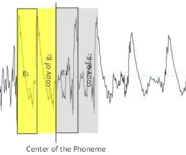
In AS1, after the detection of a phoneme, a

segment of 25 milliseconds is extracted from the sample, as shown in Fig. 1. This segment has two parts: one to the left side and second part to the right side of the center of the phoneme, and they are named as g1 and g2, respectively. The length

of each part of the segment is the same, 12.5 milliseconds. Before pasting the extracted segment, the whole speech signal at the right side of g2 is shifted, for the same amount of time (i.e.

25 milliseconds) to make room for the extracted segment. The newly generated sample after applying AS1 is shown in Fig. 2.

∑

= _iM₁wig(X|μi,Σi)

) | p(X λ

(

)

 



_{− − −}

=

_∑

i i

' i 2

1 i 2 D i

i (X μ) (X μ)

2 1 exp Σ 2

1 ) Σ , μ | g(X

448

4.1.2 Second lengthening method AS2

In AS2, a segment is extracted and pasted in the

same way as in the method AS1 but its length is 50

milliseconds and the length of each part, g1 and g2 ,

is 25 milliseconds.

4.1.3 Third lengthening method AS₃

In this method, a segment of 50 milliseconds is extracted from the original training sample in the same way as extracted by using AS2 but pasted in

a different way. Both parts of the extracted sample g1 and g2 have 25 milliseconds length each. After

extraction of the segment, its left part g1is pasted

just after the place it was copied from and the rest of the sample is shifted towards its right. Similarly, the second part g2 of the extracted segment is

pasted where g2 ends. This technique is labeled as

AS3. Extraction of the segment and its pasting in

the sample by using the method AS3 is shown in

Fig. 3 and Fig. 4, respectively.

Figure 1: Extraction of Segment by using the method AS1

Figure 2: Sample after Appending the Extracted Segment by using AS₁

4.2. Adding Noises at Different SNRs

Different samples are generated by adding two types of noise i.e. Babble Noise (BN) and Train Noises (TN) in the original training samples w1A

and w1B. These noises are added at SNRs of 5 dB,

10 dB and 15dB. The purpose of this technique is to simulate different environments around the speaker and/or different recording equipment

.

Figure 3: Extraction of Segment from the Signal by using AS3

Figure 4: Sample after Appending the Extracted Segment by using AS₃

4.3. Word Reversing and its Lengthening

In this technique, samples are generated by reversing the original samples and different methods of the lengthening are applied on the generated reversed samples.

5. SAMPLES GENERATION AND

EXPERIMENTS BY USING ONE SAMPLE

449 training sample w1A. The experiments are

performed by considering the three different subsets of the database; these are subsets A, B, and C which contain 50, 37 and 78 speakers, respectively.

5.1. Samples Generation from the First Original

Sample w_1A

Six new samples are generated by applying the method AS1 and AS2 on the sample w1A. As

discussed in section 2, original speech sample w1A

contains three phonemes [ﻥ], [ﻉ] and [ﻡ]. The samples, say w2, w3 and w4, are generated by

applying AS1 on the sample w1A. The sample w2 is

generated after automatic detection of the phone [ﻥ], and then the segment containing middle of the phone is extracted and pasted into w1A. Similarly,

samples w3 and w4 are generated by detecting [ﻉ]

and [ﻡ] respectively and then the segment containing middle of the phone is extracted and pasted in w1A.The lengthening techniques AS2 is

applied on w1A to generate three more generated

samples, named as w5, w6 and w7. The lengthening

techniques AS3 is applied on w1A to generate three

more generated samples, named as w34, w35 and

w36.

Babble noise of 5 dB, 10 dB and 15 dB SNR is added to the original training sample w1A which

produces three samples w8, w9 and w10

respectively. Three more samples, referred to as w11, w12 and w13 are generated by adding train

noise at the three levels of SNRs.

The samples w15, w16, w17 are generated by

applying the lengthening technique AS1 on the

reverse of the original samples, which we called w14. By applying AS3 on w14 we get w37, w38 and

w39.

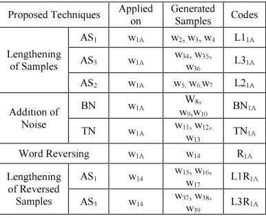
A summary of all the generated samples from the original training samples w1A with their method of generation are presented in Table 1. Different codes in the last column of the Table1 are introduced which provide the information about the generated samples. For instance, L1R1A

refers to the samples that are generated by the first method of the lengthening of sample when applied on the reverse of the sample w1A.

5.2. EXPERIMENTAL SETUP

In order to confirm that the new generated samples contain supplementary information about the speakers, two initial experiments are performed. In the first experiment, named Exp1, the system is trained with an original sample and

four copies of it, and tested with another original sample. The obtained recognition rate was 10%, as

Table 1: Summary of Samples Generated from w1A

Proposed Techniques Applied on

Generated Samples Codes

Lengthening of Samples

AS1 w1A w2, w3, w4 L11A

AS3 w1A w 34, w35,

w36 L31A

AS2 w1A w5, w6,w7 L21A

Addition of Noise

BN w1A W 8,

w9,w10 BN 1A

TN w1A w 11, w12,

w13

TN1A

Word Reversing w1A w14 R1A

Lengthening of Reversed Samples

AS1 w14 w 15, w16,

w17 L1R 1A

AS3 w14 w 37, w38,

w39

L3R1A

expected, which is very low since information contained in one sample is not sufficient for identification of the true speaker. In the second experiment, named Exp2, the system is trained with four generated samples and tested with the original sample of these samples, and we obtained 100% recognition rate. This result is obtained due to supplementary or additional information obtained during the training of the system by the new generated samples. However, this is not a real test, because the system should be tested with other original samples.

To evaluate the performance of the proposed techniques, all experiments are performed on two types of the recognition system. Both systems use MFCC as a feature extraction technique to capture the speaker dependent characteristics but differ in modeling techniques. The first system uses HMM and the second uses GMM to construct the acoustic models of speakers. The systems are trained by using the first original sample w1A and

different combinations of the samples generated from w1A, and tested with the remaining original

samples w1B, w1C, w1D, and w1E. Each combination

of the generated samples is represented by a group. The list of these groups with training and testing samples is presented in Table 2.

5.3. Results when using One Original Sample

450

Table 2: List of the Groups for the Training

Group Training samples Testing samples G1 w1A, L11A

w1B, w1C,

w1D, w1E

G2 w1A, L21A

G3 w1A, L11A, L21A

G4 w1A, L11A, L21A, R1A

G5 w1A, L11A, L21A, L1R1A

G6 w1A, L11A, L1R1A

G7 w1A, L11A,BN1A

G8 w1A, L11A, BN1A , TN1A

G9 w1A, L11A,TN1A

G10 w1A, L21A,BN1A

G11 w1A, L21A,TN1A

G12 w1A, L21A, BN1A , TN1A

G13 w1A, L11A, L21A,BN1A

G14 w1A, L11A, L21A,TN1A

G15 w1A, L11A, L21A,BN1A , TN1A

G16 w1A, L11A, R1A

G17 w1A, L21A, R1A

G18 w1A, , L21A,, L1R1A

5.3.1. HMM results for the subset A

The recognition rates of the groups G1, G2, G3, G4, G5, G6, G7 and G8 by using HMM based speaker recognition system are presented in Table 3. Every time one of the groups is used to train the system for the speaker recognition task and the system is tested by the four original samples w1B,

w1C, w1D, w1E. The database is subset A which has

50 speakers

.

Table 3: Recognition Rates (%) for HMM

Groups Recognition Rates

G1 85

G2 79.40

G3 88

G4 69.70

G5 67.17

G6 71.72

G7 68.90

G8 77.78

A comparison of results of the groups is provided in Fig.5. The groups are aligned in descending order of their recognition rates along the X-axis and their recognition rates in percentage

are along Y-axis. The recognition rate of group G3, which is 88%, is better than that of groups G1 and G2. Group G3 is using the combination of the methods AS1 and AS2, while G1 and G2 are using

method AS1 and AS2 respectively. The result of

group G8 which uses both types of noise at different SNRs is also encouraging as compared to G7 which has only one type of noise. But groups G4, G5 and G6, obtained by applying word reversing and its lengthening, did not show promising results.

Figure 5: Comparison of Groups for HMM.

5.3.2. GMM results for the subset A

To evaluate the accuracy of the proposed technique, different experiments are performed by using GMM, while speaker dependent properties are captured by using MFCC. The experiments show that variation in number of MFCCs and number of GMM mixtures affects the recognition rate, as presented in Table 4 and Table 5. The results in these tables are found by using 12 and 36 MFCCs with 4, 8, 16 and 32 GMM mixtures. The database is the subset A that has 50 speakers.

Table 4: Recognition rate (%) for Subset A with 12 MFCCs

Group

12MFCC 4

GMM 8 GMM

16 GMM

32 GMM G1 78.00 74.00 64.00 46.00 G2 77.50 80.50 79.00 64.00 G3 79.00 74.00 73.00 55.00 G4 80.81 81.82 76.26 53.03 G5 87.88 83.33 82.32 74.75 G6 85.35 77.78 77.78 63.13 G7 77.78 80.30 73.23 63.13 G8 87.88 89.90 84.34 65.66

Table 5: Recognition rate (%) for Subset A with 36 MFCCs

Group

36MFCC 4

GMM 8 GMM

16 GMM

32 GMM G1 79.00 60.00 47.00 28.00 G2 77.50 63.50 46.50 35.50 G3 83.00 75.00 60.00 37.00 G4 76.77 69.19 59.60 38.89

R

e

c

o

gn

it

io

n

R

at

e

(

%

)

451

G5 89.39 78.28 70.71 46.97 G6 77.78 66.16 62.63 42.42 G7 71.21 56.06 43.94 20.20 G8 88.38 84.85 71.72 50.00

Comparisons of the results of all the above groups when using different number of GMM mixtures are depicted in Fig. 6 and Fig. 7. Recognition rates with 12 MFCCs are presented in Fig. 6 and that of with 36 MFCCs are provided in Fig. 7. Recognition rates for 4 and 8 GMM mixtures with 12 MFCCs are almost same. But recognition rate with 4 mixtures clearly outperform the 8, 16 and 32 mixtures for 32 MFCCs. For higher number of mixtures, recognition rates decrease as compared to 4 and 8 mixtures, for all MFCCs.

The highest recognition rates for the method AS1 (group G1) and AS2 (group G2) are 79% and 80.50%, respectively. The system parameters for G1 are 4 mixtures and 36 MFCCs, and for G2, parameters are 8 GMM and 12 MFCCs. The highest recognition rate for word reversing and its lengthening is 89.39%, when the technique is used with the combination of AS1 and AS2 (group G5), with 4 mixtures and 36 MFCCs. The recognition rate of 89.90% is obtained when both types of noise, babble and train noise, are combined with the method AS1. This result is obtained for group G8 with 8 mixtures and 12 MFFCs. It is the maximum result achieved by using GMM for any group and is a 1.90% improvement as compared to HMM result.

By comparing the results of HMM and GMM we see that GMM is better overall. Therefore, in the rest of the paper we will use only GMM.

Figure 6: GMM Recognition Rate with 12 MFCC

Figure 7: GMM Recognition Rate with 36 MFCC

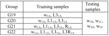
To test the method AS3 some more experiments

are performed with the new groups, G19 to G22, as presented in Table 6. In these groups lengthening technique AS3 and/or other proposed

techniques are used to generate new samples. The recognition rates for groups, G19 to G22, are presented in Table 7 and Table 8 for 12 and 36 MFCC, respectively.

Table 6: Groups of the First Approach with AS₁and AS3

Group Training samples Testing _samples G19 w1A, L31A

w1B, w1C,

w1D, w1E

G20 w1A, L11A, L31A

G21 w1A, L11A, L31A, R1A

G22 w1A, L11A, L31A, L3R1A

Table 7: Recognition rate (%) for Subset A with 12MFCCs

Groups

12MFCC 4

GMM 8 GMM

16 GMM

32 GMM G19 79 79 78 60 G20 82 79.5 79 58 G21 80.30 81.31 77.78 60.61 G22 85.35 78.28 76.26 56

Table 8: Recognition rate (%) for Subset A with 36 MFCCs

Groups

36MFCC 4

GMM 8 GMM

16 GMM

32 GMM G19 82 72 64 47 G20 77.78 74.75 52.02 37.37 G21 78 71.50 57.50 28.50 G22 77.78 68.69 64.14 49.49

The recognition rate for the group G19, using the method AS3, is 82% with 4 mixtures and 36

MFCCs, showing improvement of 3% and 4.50% as compared to G1(using AS1) and G2 (using

AS2), respectively, with same parameters. The

452 combination of AS1 and AS3 for samples

generation, while G3 is using combination of AS1

and AS2.

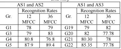
In tables 7 and 8, the results are higher when 4 mixtures are used; hence, in Table 9, the results of the groups using AS1 and AS2 with the results of the corresponding groups using AS1 and AS3 are compared, all using 4 mixtures.

Table 9: Comparison of AS1 and AS2with AS1 and AS3

and AS3

AS1 and AS2 AS1 and AS3

Gr.

Recognition Rates Gr.

Recognition Rates 12

MFCC 36 MFCC

12 MFCC

36 MFCC G1 78 79 G19 79 82 G3 79 83 G20 82 77.78 G4 80.8 76.8 G21 80.30 78 G5 87.9 89.4 G22 85.35 77.78

From the previous discussion and from Table 9 we can see that there is no significant improvement in the recognition rates for technique AS3 as compared to AS1 and AS2 for other groups.

This is the reason that we conduct the rest of the experiments by using those groups that are generated by using AS1 and AS2.

5.3.3. GMM results for the subset B

All groups of Table 2 are evaluated for the subset B which contains only male speakers. The results of all groups with different number of GMM mixtures with 12 MFCC features are presented in Table 10 and that of with 36 MFCC are provided in Table 11.

The average results of all the groups for 4, 8, 16 and 32 mixtures with 12 MFCCs are 98.50%, 98.65%, 98.35% and 97%, respectively, and that of with 36 MFCCs are 98.46%, 98.01%, 97.15% and 92.27%.There is no significant difference in the averages for all number of mixtures with 12 MFCCs but for 36 MFCCs average with 32 mixtures is significantly down as compared to the others.

Table 10: Recognition rate (%) for Subset B with 12 MFCCs

Group

12MFCC 4

GMM 8 GMM

16 GMM

32 GMM G1 99.32 98.65 98.65 94.59

G2 98.65 98.65 97.30 85.81

G3 97.97 97.97 97.30 91.22

G4 98.65 99.32 97.97 99.32

G5 97.97 98.65 98.65 97.97

G6 98.65 98.65 98.65 97.97

G7 98.65 98.65 99.32 98.65

G8 97.97 98.65 97.97 97.30

G9 98.65 97.97 98.65 98.65

G10 97.97 98.65 97.97 97.30

G11 97.97 98.65 98.65 99.32

G12 98.65 98.65 99.32 98.65

G13 97.97 98.65 98.65 97.97

G14 98.65 98.65 98.65 97.97

G15 98.65 99.32 97.97 99.32

G16 99.32 98.65 97.97 97.97

G17 98.65 98.65 97.97 98.65

G18 98.65 98.65 98.65 97.30

Table 11: Recognition rate (%) for Subset B with 36 MFCCs

Group

36MFCC 4

GMM 8 GMM

16 GMM

32 GMM G1 97.97 93.92 92.57 79.73

G2 97.97 96.62 93.92 81.08 G3 97.97 97.97 93.92 74.32

G4 98.65 98.65 98.65 96.62

G5 97.97 97.97 98.65 97.97

G6 98.65 98.65 98.65 96.62

G7 98.65 97.97 97.30 94.59

G8 98.65 98.65 98.65 95.27

G9 98.65 97.97 97.30 93.92

G10 98.65 98.65 98.65 93.24

G11 98.65 98.65 97.97 90.54

G12 98.65 98.65 97.97 96.62

G13 98.65 97.97 97.30 93.24

G14 98.65 97.97 96.62 91.89

G15 97.97 98.65 97.97 96.62

G16 99.32 97.97 97.97 95.95

G17 98.65 98.65 97.30 95.95

G18 97.97 98.65 97.30 96.62

The maximum recognition rate for 12 MFCCs is 99.32% for 9 different groups as highlighted in Table 10. The highest recognition rate for 36 MFCCs is 97.97% and it comes with 32 mixtures for group G5.

5.2.3. GMM results for the subset C

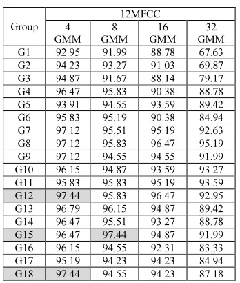
The performance of all the groups of Table 2 when using subset C is provided in the Table 12 and Table 13 for 12 MFCCs and 36 MFCCs, respectively, with different number of GMMs.

453 G15 and G18. The highest rate for 36 MFCCs is 97.76% which is obtained for the group G12. This group contains samples generated by addition of babble and train noise and second method of lengthening.

Table 12: Recognition rate (%) for Subset C with 12 MFCCs

Group

12MFCC 4

GMM 8 GMM

16 GMM

32 GMM G1 92.95 91.99 88.78 67.63 G2 94.23 93.27 91.03 69.87 G3 94.87 91.67 88.14 79.17 G4 96.47 95.83 90.38 88.78 G5 93.91 94.55 93.59 89.42 G6 95.83 95.19 90.38 84.94 G7 97.12 95.51 95.19 92.63 G8 97.12 95.83 96.47 95.19 G9 97.12 94.55 94.55 91.99 G10 96.15 94.87 93.59 93.27 G11 95.83 95.83 95.19 93.59 G12 97.44 95.83 96.47 92.95 G13 96.79 96.15 94.87 89.42 G14 96.47 95.51 93.27 88.78 G15 96.47 97.44 94.87 91.99 G16 96.15 94.55 92.31 83.33 G17 95.19 94.23 94.23 84.94 G18 97.44 94.55 94.23 87.18

Table 13: Recognition rate (%) for Subset C with 36 MFCCs

Group

36MFCC 4

GMM 8 GMM

16 GMM

32 GMM G1 93.27 84.94 62.18 51.28 G2 93.27 82.69 74.68 43.91 G3 93.27 89.42 75.96 45.83 G4 96.79 95.19 80.13 64.10 G5 95.51 95.51 95.51 90.38 G6 96.79 94.87 93.27 79.81 G7 95.19 92.31 89.10 73.40 G8 97.12 96.15 93.27 83.33 G9 94.87 94.55 87.50 79.17

G10 96.79 91.67 90.06 76.60

G11 94.87 92.95 83.33 69.23

G12 97.76 97.44 92.63 85.26

G13 97.44 91.99 88.46 64.42

G14 94.87 94.23 80.45 65.38

G15 96.79 94.23 91.03 85.58

G16 96.15 94.23 88.14 70.19

G17 95.51 96.15 91.67 76.28

G18 96.47 96.15 92.31 86.22

6. SAMPLES GENERATION AND EXPERIMENTS BY USING TWO SAMPLES

Sixteen more samples are generated from the second original sample w1B to enhance the number

of samples in the database. These samples are used with the samples generated from w1A to train the

system. The performance of the proposed techniques is evaluated by using subset A of the database which contains children, females and males.

6.1. Sample Generation from Second Original

Sample w1B

Six different samples are generated by applying the techniques AS1 and AS2 on the sample w1B one

by one. These samples are w18, w19, w20, w21, w22

and w23, and are generated in the same way as in

previous section for samples w1, w2, w3, w4, w5,

and w6 from the original sample w1A. SNR levels

of 5dB, 10dB and 15dB for both types of noise, babble and train, are added to the sample w1B to

generate the new samples w24, w25, w26, w27, w28

and w29. The new sample w30 is generated by

reversing the sample w1B. At the end, three more

samples w31, w32 and w33 are obtained from w30

after applying AS1. The generated samples are

presented in Table 14.

Table14: Summary of Samples Generated from w1B

Proposed Techniques Applied on

Generated Samples Codes

Lengthening of Samples

AS1 w1B w 18, w19,

w20 L1 1B

AS2 w1B

w21,

w22,w23 L21B

Addition of Noise

BN w1B w 24,

w25,w26 BN 1B

TN w1B w 27, w28,

w29

TN1B

Word Reversing w1B W30 R1B

Lengthening of Reversed Samples

AS1 W30 w 31, w32,

w33 L1R1B

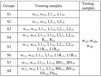
6.2. Experimental Setup

Two original samples w1A and w1B and their

corresponding generated samples are used for the training and the remaining three original samples w1C, w1D, w1E are used for the testing. The methods

AS1 and AS2 are used individually or their

454

Table 15: Groups of the Second Approach with Training and Testing Samples

Groups Training samples Testing _samples S1 w1A, w1B, L11A, L11B

w1C,w1D,

w1E S2 w1A, w1B, L21A, L21B

S3 w1A, w1B, L11A, L11B, L21A, L21B

S4 w1A, w1B, L11A, L11B, L21A, L21B,

R1A, R1B

S5 w1A, w1B, L11A, L11B, L21A, L21B,

L1R1A, L1R1B

S6 w1A, w1B, L11A, L11B, L1R1A, L1R1B

S7 w1A, w1B, L11A, L11B, BN1A, BN1B

S8 w1A, w1B, L11A, L11B, BN1A, BN1B,

TN1A,TN1B

6.3. Results by using Two Original Samples

All experiments are performed by using GMM based recognition system for subset A of the database and the results are provided in Table 16 and Table 17. The recognition rates of Table 16 and Table 17 are obtained by using 4, 8, 16 and 32 mixtures with 12 MFCCs and 36 MFCC, respectively.

Table 16: Recognition rate (%) for Subset A with 12 MFCC

Groups

12 MFCC 4

GMM 8 GMM

16 GMM

32 GMM S1 100 100 99.33 94.67 S2 100 98.67 100 98.67 S3 99.33 98.67 98.67 93.33 S4 100 100 99.33 95.33 S5 100 100 98.67 95.33 S6 100 100 100 95.33 S7 100 100 100 97.33 S8 100 100 100 98.67

Table 17: Recognition rate (%) for Subset A with 36 MFCC

Groups

36 MFCC 4

GMM 8 GMM

16 GMM

32 GMM

S1 96 96 84.67 68

S2 98.67 92 90 68.67

S3 96.67 92 85.33 66.67

S4 100 98.67 98.67 94

S5 100 100 100 98.67

S6 100 100 99.33 95.33

S7 98.67 91.33 80 66.67

S8 99.33 95.33 93.33 74

By analyzing Table 16 and Table 17, it is concluded that recognition rates for 4 mixtures outperforms 8, 16 and 32 mixtures for all numbers of MFCCs. Recognition rates for 12 MFCCs are better than 32 MFCCs most of the time. Moreover, training with two original samples provides much better result than training with one original sample.

In the experiments that use one training sample, the groups G1, G2 and G3 have 78%, 77.50% and 79%, respectively, with 12 MFCCs and 4 GMM. The methods AS1 and AS2 are used in the groups

G1and G2, respectively, and a combination of AS1

and AS2 is used in G3. While in the experiments

that use two training samples, recognition rates of the groups S1, S2 and S3 are 100%, 100% and 99.33%, respectively, with 12 MFCCs and for 4 mixtures. The methods AS1, AS2 and their

combination is used in the groups S1, S2 and S3 respectively. Hence, training by using two original samples performed well as compared to one sample.

The groups G4, G5 and G6 have same methods of generation as S4, S5, and S6. Recognition rate of each of the groups S4, S5, S6 is 100% which is much higher than the recognition rate of groups G4, G5 and G6. The group G5 has maximum recognition rate, which is 89.39% for 36 MFCCs and 4 mixtures. Furthermore, the recognition rates of all the groups Gi and Si, where i = 1, 2, 3 …, 8, when using 12 MFCCs are better as compared to when using 36 MFCCs; and 4 mixtures again outperforms 8, 12 and 32 mixtures.

Babble noise is added in the samples of group S7 and they are used with the samples generated by the method AS1 for training of the developed

system. While in group S8, two types of the noise, Babble and Train Noises, are added in the samples and they are used with the samples generated by the methods AS1 and AS2. The recognition rates

for both groups are 100%.

7. COMPARING THE PERFORMANCE OF THE MANUAL AND AUTOMATIC

LENGTHENING TECHNIQUES

455 the paper which had the result of the manual technique [11], so in the three Tables 18, 19, and 20, we compare the results of the group in this paper with the corresponding group in [11].

From Table 18, we can see that the manual and automatic techniques had a similar overall performance. Table 19 presents the result when using subset A. We can see that the manual technique performs better, while at many instances they were near. The maximum rate for manual method is 91.4% and maximum rate for automatic method is 89.4 %, obtained at same configuration. From Table 20, presenting the result when using subset B, the automatic technique had an excellent performance, 97.97- 99.32 and it was always higher than the manual technique, around 8%.

Table 18. Performance Comparison of the Manual and Automatic techniques when using HMM and Subset A

Manual Automatic

Groups Recognition

Rates Groups

Recognition Rates

L1 70 G1 85

L2 63 G2 79.40

L3 83 G3 88

R5 87 G4 69.70

R6 90 G5 67.17

R2 88 G6 71.72

N1 75 G7 68.90

N3 72 G8 77.78

Table 19. Performance comparison of the Manual and Automatic techniques when using GMM and Subset A

Manual Automatic

Groups

Recognition Rates

Groups

Recognition Rates 12

MFCC 36 MFCC

12 MFCC

36 MFCC

L1 79 83.8 G1 78.00 79.00 L2 87 87.5 G2 77.50 77.50 L3 90 82.8 G3 79.00 83.00 R5 88 89 G4 80.81 76.77 R6 89 91.4 G5 87.88 89.39 R2 88.9 88.9 G6 85.35 77.78 N1 88.9 85.4 G7 77.78 71.21 N3 88.4 88.9 G8 87.88 88.38

Table 20. Performance Comparison of the Manual and Automatic techniques when using GMM and Subset B

Manual Automatic

Groups

Recognition Rates

Groups

Recognition Rates 12

MFCC 36 MFCC

12 MFCC

36 MFCC

L1 91.2 90.5 G1 99.32 97.97 L2 90.5 90.5 G2 98.65 97.97 L3 89.2 90.5 G3 97.97 97.97 R5 93.2 90.5 G4 98.65 98.65 R6 92.6 89.9 G5 97.97 97.97 R2 91.2 90.5 G6 98.65 98.65

N1 91.2 91.2 G7 98.65 98.65 N3 91.2 92.6 G8 97.97 98.65

8. CONCLUSION AND FUTURE WORK

In this paper, different automatic techniques for corpus expansion are proposed to enhance the speaker information in new generated samples. These automatic techniques are: lengthening of sample by automatic segmentation, addition of noise at different SNRs and, word reversing and its lengthening. The lengthening of sample is applied by using three different methods. These methods differ either by length of the extracted segment or by the way of copying and pasting of the segment into the original sample.

Two different approaches are used to train the system. In the first approach, the system is trained by using one original sample and its generated sample. In the second approach, two original samples and its generated samples are used to train the system.

We evaluated the techniques using three subsets of the database. Subsets A, B, and C have 50 (male and female), 37 male, and 73 male speakers, respectively.

Using GMM is easier and faster than using HMM and the results of both are similar; hence for most of the paper we used GMM as the modeling technique. The obtained results are very encouraging. For the first approach, using one original sample, the maximum recognition rate was 89.4, 99.2%, and 97.4% for subsets A, B, and C respectively (using 4 mixtures). For the second approach, using two original samples, the results were excellent. The maximum recognition rate was 100% at many of the combinations, particularly, for 12 MFCC. It is to be noted that the result of both approaches and for all the combinations were maximum when using only 4 mixtures.

It can be concluded that proposed techniques presented in this paper can handle the hard situation in which only one or two samples of the speaker is available to train the system. Moreover, the complete process of segmentation and, training and testing of the system is automatic. Therefore, our approach can be deployed for the surveillance and security measures when little amount of information is available to recognize a person.

456

ACKNOWLEDGMENTS

This work is supported by the National Plan for Science and Technology in King Saud University under grant number 13-INF977-02. The authors are grateful for this support.

REFERENCES:

[1] J. P. Campbell, et al., “Forensic speaker recognition: a need for caution,” IEEE Signal Processing Magazine, March 2009, pp. 95-103.

[2] L. Breiman, “Bagging Predictors”, Technical Report No. 421, Dept. of Statistics, University of California (Berkley). Sept 1994.

[3] L. Breiman, “Bagging Predictors”, Machine Learning, Vol. 24, Springer Netherlands, 1996, pp 123-140.

[4] Lean Yu, Shouyang Wang, Kin Keung Lai, “Credit risk assessment with a multistage neural network ensemble learning approach”,

Expert Systems with Applications, Vol. 34, Issue 2, February 2008, pp. 1434-1444. [5] B. Drapper and K. Baek, “Bagging in

Computer vision”.CVPR, pp. 144-149, 1998. [6] Leo Breiman, Random Forests, Machine

Learning, v.45 n.1, October 1, 2001, pp. 5-32.

[7] Leo Breiman, “Using Iterated Bagging to Debias Regressions”, Machine Learning, v.45 n.3, December 2001, pp. 261-277. [8] M. Mori, A. Susuki, A.Shio and S. Othsuka,

“Generating new samples from handwritten numerals based on point correspondence”.

Proceedings of the 7th IWFHR, Amsterdam, Netherlands, 2000, pp. 281-290.

[9] Li Fei-Fei, R. Fergus, P. Perona, “Learning Generative Visual Methods from few training Examples: An incremental Bayesian Approach tested on 101 Object categories”,

Computer vision and Image understanding,

V. 106, issue 1, 2007, pp. 59-70.

[10] M. Alsulaiman, A. Mahmood, M. Ghulam, M. A. Bencherif, and Y. Alotaibi, “A Technique to Overcome the Problem of Small Size Database for Automatic Speaker Recognition”, Proceeding of Fifth International Conference on Digital Information Management, Thunder Bay, Canada 2010, pp. 303-308.

[11] M. Alsulaiman, “A technique to overcome the problem of small size database for

automatic speaker recognition”,

International Journal of Physical Sciences, March 2012, Vol. 7(13), pp. 2076 – 2084. [12] M. Alsulaiman, “Automatic Enlargement of

Speech Corpus for Speaker Recognition”,

Proceeding of 2011 IEEE Symposium on Computer & Informatics, March 2011, pp. 302-306.

[13] C. Jianfen, “Restudy of segmental lengthening in Mandarin Chinese,”

Proceeding of Speech Prosody 2004, Nara, Japan, pp. 231-234.

[14] O. Erogul and I. Karagoz, “Time-scale modification of speech signals for language-learning impaired children,” Proceeding of the 2nd International Biomedical Engineering Days, 1998, pp. 33-35.

[15] S. Roucos and A.M. Wilgus, “High Quality Time-Scale Modification for Speech”,

Proceeding of the IEEE Int. Conf. Acoust. Speech, Signal Process., ICASSP-85, 1985, pp. 493-496.

[16] E. Moulines and F. Chanpentier,

“Pitch-Synchronous Waveform Processing

Techniques for text-to-Speech Synthesis Using Diphones”, Speech Communication, vol. 9, 1990, pp. 453-467.

[17] S.S. Al-Dahri, Y.H. Al-Jassar,Y.A. Alotaibi, M.M. Alsulaiman, K.A.B Abdullah-Al-Mamun, “A Word-Dependent Automatic Arabic Speaker Identification System”

Proceeding of IEEE Signal Processing and Information Technology, ISSPIT 2008, pp. 198-202.

[18] L. Rabiner and B.H. Juang, Fundamentals of speech recognition. Englewood Cliffs, NJ: Prentice-Hall, 1993.

[19] Z. Ali, M. Aslam, A. M. Martinez Enriquez, “A Speaker Identification System using MFCC Features with VQ Technique”,

Proceeding of the 3rd International Symposium on Intelligent Information Technology Application, 2009, pp. 115-119. [20] Z. Razak, N. J. Ibrahim, M. Y. IdnaIdris, et

al.,“Quranic Verse Recitation Recognition Module for Support in J-QAF Learning: A Review”, International Journal of Computer Science and Network Security (IJCSNS), August 2008, vol. 8, No.8, pp. 207-216,

457 [22] T.Matsui, S.Furui, “Comparison of

text-independent speaker recognition methods using VQ-distortion and discrete/continuous HMMs”, Proceeding of ICASSP, 1992, pp. II.157-164.

[23] Z. Ali, M.Aslam, M. E.Ana María, GonzaloE., “Text-independent speaker identification using VQ-HMM model based multiple classifier system.”, Lecture Notes in Computer Science, Springer, Vol. 6438, pp.116-125, 2010.

[24] D. A. Reynolds and R. C. Rose, “Robust text-independent speaker identification using Gaussian mixture models,” IEEE Trans. Speech Audio Process., 1995, Vol. 3, No. 1, pp. 72–83.

[25] B. L. Pellom and J. H. L. Hansen, “An efficient scoring algorithm for Gaussian

mixture model based speaker

identification,” IEEE Signal Process. Lett., 1998, Vol. 5, No. 11, pp. 281–284, Nov. 1998.