Munich Personal RePEc Archive
Bayesian Estimation of Dynamic
Stochastic General Equilibrium Model
Using UK Data
Kamal, Mona
17 February 2011
Online at
https://mpra.ub.uni-muenchen.de/29239/
1
Bayesian Estimation of Dynamic Stochastic General
Equilibrium Model Using UK Data
1
Mona Kamal
M.Sc in Economics
Queen Mary, University of London
E-mail:
[email protected]
February 17, 2011
Abstract
This paper applies the Bayesian method to estimate a Dynamic Stochastic General Equilibrium (DSGE) model using quarterly data for the UK over the period from 1971:Q1 through 2009:Q2. The contribution of the paper is two-fold. First, we estimate a model characterised by nominal and real frictions. This estimation allows us to recover the structural parameters of the economy and study the transmission mechanism of a government spending shock. Second, we investigate how the inclusion of fiscal policy rules affect the propagation of shocks and the ability of the model to fit the data. We establish that this inclusion enable the model to fit the data more closely. In addition, it has an impact on the qualitative responses of macroeconomic variables to the government spending shock.
Keywords: The transmission mechanism of a government spending shock, Bayesian analysis, (DSGE) model.
JEL Classifications: C01, C8, C83, E6, E60.
1
2
1.
Introduction
Interest in the estimation of Dynamic Stochastic General Equilibrium (hereafter DSGE) models has been heightened in recent years due to advances in macroeconometrics. A review of the empirical literature shows a wide range of approaches in the analysis of (DSGE) models. First calibration, as for example in the seminal work of Kydland and Prescott (1982). Second, applying the Generalalized Method of Moments (GMM) estimation of particular equilibrium relationships as in Christiano and Eichenbaum (1992). Third, incorporating a minimum distance estimation based on the difference between Vector Autoregression (VAR) and (DSGE) models impulse response functions as in Rotemberg and Woodford (1997), Del Negro and Schorfheide (2004), and Christiano et al. (2005). Fourth, using the Classical Maximum Likelihood Estimation (CMLE) as in Altug (1989), McGrattan (1994), Leeper and Sims (1994), Kim (2000) and Ireland (2004). Fifth, the Bayesian estimation method.2
The application of Bayesian techniques to the estimation of a (DSGE) model has been firstly done by DeJong et al. (2000). Many other researchers utilized this method for several applications, for instance: Schorfheide (2000) has compared the fit of various models using this technique, Smets and Wouters (2003, 2007) (hereafter SW) have applied Bayesian estimation techniques to a model of the Euro zone and the US. They have argued that their middle-scale (DSGE) model is almost as good at explaining the actual economy as (VAR). Fernandez-Villaverde and Rubio-Ramirez (2004) have compared estimation results with maximum likelihood and Bayesian Vector Autoregression (BVAR) methodologies. Galí and Monacelli (2005), Lubik and Schorfheide (2005) have applied this method to an open macro model focussing on issues of misspecification and identification. Rabanal and Rubio-Ramirez (2005) have compared the fit of models based on posterior distributions of four competing specifications of New Keynesian monetary models with nominal rigidities, Lubik and Schorfheide (2007) have investigated whether central banks in small open economies respond to exchange rate movements. In addition, An and Schorfheide (2007) have provided a comprehensive overview of Bayesian methods used for (DSGE) models estimation.
Despite the growing number of studies on Bayesian estimation of (DSGE) models, almost no attention is paid to fiscal policy assessment in the UK. Therefore, this paper investigates the possibility of using this type of models for the purpose of fiscal policy analysis. We claim that in order to be able to use (DSGE) models for fiscal policy analysis we need to include the actual data for fiscal policy variables in the estimated model since the analysis should be influenced by data. This in turn can be done by incorporating a fiscal policy feedback equation or an estimated fiscal policy rule.
A sequence of steps is done in this paper to reach this target. We consider the (SW, and CEE models) as the starting point using quarterly data for the UK and applying the Bayesian method. Then, we compare the results with a modified version of the model which includes the actual data for government spending and a government spending feedback rule.
2
3
Since proper modelling of government’s financing behaviour through using data is important to assess the quantitative effects of fiscal policy. The objectives of estimating the New Keynesian Dynamic Stochastic General Equilibrium (hereafter NKDSGE) model using different periods are the following. Firstly, to assess the effect of fiscal policy reforms on the economy. Secondly, to check whether the inclusion of actual data of a fiscal variable in Bayesian estimation of (DSGE) models could improve the model fit compared to an estimated version using the standard set of variables and the same sample. Thirdly, to analyze the impulse responses of macroeconomic variables to fiscal policy shocks. Fourthly, to compare the results obtained from different versions of the estimated model.
The above objectives seem to be unattainable if we take into consideration the recent contribution by Chari et al. (2009). They have claimed that (SW’s model) can not be used for policy analysis since it does not generate the type of wedges that can be seen in the data from interpretable shocks (i.e. the price and wage mark-up shocks). However, in this paper we are opponent to this point of view since the importance of those types of models depends on their ability to compete with Bayesian Vector Autoregression (BVAR) models in out-of-sample prediction which represents the main concern of policymakers.
On the contrary, we think that those models will still play the key role in policy analysis in the coming two decades, due to their prediction characteristics and the inclusion of actual data in estimation. Furthermore, it is essential to incorporate enough number of shocks to produce a nondegenerate system which can be used for policy analysis. Without the inclusion of sufficient number of structural shocks, there is no conclusion can be drawn from the model.
This paper is organized as follows. Section 2 provides a review of the relevant literature. Section 3 illustrates the estimation methodology. Section 4 discusses the model version with a fiscal policy rule. Section 5 reports the steps followed for estimation and the choice of priors. Section 6 indicates the main results and provides a model comparison. Finally, section 7 concludes.
2.
Review of the Literature
(NKDSGE) models are widely used in monetary policy analysis by many central banks nowadays and the art of modelling the economy using those types of models is evolving given the development in Bayesian methods. Indeed, a version of the (SW model) is now being used to inform policymaking at the European Central Bank (ECB). Most of the empirical work is applied to the US and the Euro Zone, and concentrates mainly on the analysis of the business cycles, productivity and monetary policy shocks in different regimes.
(SW, 2003, 2007) have showed that modern micro-founded (NKDSGE) models with sticky prices and wages along the lines developed by Christiano et al. (2005) are rich to capture most of the statistical features of the main macroeconomic time series. Therefore, applying Bayesian estimation techniques will reduce relatively large models to an estimated system that provides values to the structural shock processes driving important input in the monetary policy decision process. Surprisingly, there is no equivalent research for fiscal policy analysis.
Regarding the UK, a review of macroeconomic modelling reveals the following episode, in the 1980s, a generation of macro models emerged that attempted to respond to the Lucas critique directly with the use of rational expectations econometrics (e.g. Andrewset al. (1986), Fisher et al. (1987), (1990), and Church
4
On the other hand, the introduction of (VAR) models in macroeconometrics came around the same time. The seminal work by Sim (1980) has motivated further estimation using (VARs) and (SVARs) approaches. Another approach has been applied by Garratt et al. (2003, 2006) who have used the structural cointegrating (VAR) approach where the estimated long-run relationships embodied in the model are consistent, and have a clear economic interpretation, and the short-run dynamics are flexibly estimated within a (VAR) framework. However, the role of fiscal policy has been discarded in their analysis.
The following table reflects the direction of the immediate response of private consumption, output, real wages and private investment to a positive government spending shock using different identification approaches of the VAR.
Table (1): The Impact of a Government Spending Shock on the Main Macroeconomic Variables in the UK using VAR approach
The Identification Method Consumption Output Real wages Investment
Using a Bayesian Structural Vector Autoregression (BSVAR) model
Afonso and Sousa (2009)
( no response) ↓ ↑ ↓
Using SVAR and Panel VAR, respectively
Monacelli and Perotti (2006) and Ravn et al.
(2007)
↑ ↑ ↑
Was not of the main interest of Ravn et al.* However,Monacelli and
Perotti found a fall in investment
Using a BVAR model and applying the sign restriction identification approach as in Mountford and Uhlig (2009)
Kamal (2010) **
↓ ↑ ↓ ↑
Source: prepared by the author.
*They have indicated a deterioration of the trade balance, and a depreciation of the real exchange rate.
[image:5.612.68.552.234.593.2]5
Regarding the estimation of large-sale macroeconometrics models, a seminal contribution by Harrison et. al. (2005) (i.e. the Bank of England Quarterly Model (BEQM) represents a comprehensive analysis of all aspects of the economy). However, one limitation in using this model is its dissimilarity to the model of the US by Christiano et al. (2005) and that of SW (2003, 2007) for the Euro area and the US, respectively. Therefore, it is difficult to compare the structure of the British economy with other economies using the different structures of those models. Therefore, we claim that a medium-scale (NKDSGE) model is more appropriate for comparison and policy analysis.
Lubik and Schorfheide (2007) have estimated a small-scale, structural general equilibrium model of a small open economy using Bayesian methods. They have focused mainly on the conduct of monetary policy in the UK.3 They have considered a Taylor rule, where the monetary authority reacts to output, inflation, and exchange rate movements. They have performed posterior odds tests to investigate the hypothesis whether central banks do target exchange rates. The main result of their paper is that Bank of England (BoE) does include the nominal exchange rate as an essential variable in its policy rule. This result is robust for various specifications of the policy rule.
DiCecio and Nelson (2007) have used the model of Christiano et al.(2005) to analyze monetary policy shocks in the UK using a minimum-distance estimation procedure. They have found that price stickiness is an important source of nominal rigidities in the UK than wage stickiness. However, their model is a closed-economy model which does not reflect the main features of an open economy like the UK.
Moreover, Faccini (2009) et al. have estimated a (NKDSGE) model of the labour market in the UK with matching frictions and nominal wage rigidities. Harrison and Oomen (2010) have used a simpler version of the (BEQM) model, featuring many types of nominal and real frictions. They have estimated the model in two stages. First, they have evaluated a calibrated version of the stochastically singular model. Then, they have augmented the model with structural shocks motivated by the results of the evaluation stage and estimated the resulting model using UK data and applying a Bayesian approach. Their findings suggest that the shock processes play a crucial role in helping the model to match the data.
Surprisingly, there is no intensive investigation of fiscal policy shocks through applying the Bayesian estimation of a (NKDSGE) models using the UK data. Therefore, this paper fills-in this gap.
3.
The Methodology
An important advantage of Bayesian estimation is that the information from the prior is combined with the information from the likelihood and the resulting function is maximized with respect to the parameters until the combination of parameters estimates that produces the highest value for the objective function is found. In addition, this method provides a consistent way to update the parameter values based on the observed data. It incorporates information coming either from previous studies or reflecting the subjective opinions of the researcher through the specification of prior probability density functions for the parameters. The time series are then used to revise the parameter values to get posterior estimates. Furthermore, the posterior distribution corresponding to competing models can be used to determine which model best fits the data.
6
Nevertheless, (CMLE) does not incorporate such information. Another advantage of Bayesian estimation is that, it fits the complete solved (NKDSGE) model as opposed to (GMM) estimation. The Bayesian method can be illustrated as follows, priors are described by a probability density function of the form
p
(
θ
)
, whereθ
is the parameter vector. Then, the likelihood function describes the density of the observed data given the model and its parameters:( )
θYT ln(
p(YTθ))
(1)L ≡
Where
Y
T are the observations available until timeT .In order to obtain the posterior density
p
( )
θ
Y
T . The Bayes theorem indicates that the posterior density of parameters knowing the data is related to the prior and the likelihood as follows:( )
( )
( )
(
)
( )
(
2
)
)
(
)
(
T TT T T
Y
p
Y
p
Y
p
p
Y
p
Y
p
θ
=
θ
θ
∝
θ
θ
=
κ
θ
Where
p
(
Y
T)
is the unconditional data density as it does not depend on the unknown parameters it is usually neglected from estimation.κ
( )
θ
Y
T is the posterior kernel.Assuming that priors are independently distributed, the log posterior kernel can be calculated as follows:
( )
ln(
( )
)
ln( ( )) (3) ln 1 i N i TT p Y p
Y θ θ
θ
κ
∑
=
+ =
Where N is the number of the estimated parameters.
This equation is maximized with respect to
θ
in order to obtain an estimate of the mode of the posterior distribution and for the Hessian matrix evaluated at the mode. So, here arises the link between estimation and simulation since the likelihood function is estimated using a linear prediction error algorithm like the Kalman filter and then the posterior kernel is simulated using a Monte Carlo method such as the Metropolis-Hasting (MH) algorithm.This algorithm is applied in Dynare software using the following steps: firstly, we need to choose a candidate parameter
θ
* from a normal distribution with mean set toθ
t−1 . Secondly, to compute the value of the posterior kernel for that candidate parameter and compare it to the value of the kernel from the mean of the drawing distribution. Thirdly, to decide whether or not to hold on the candidate parameter by computing the acceptance ratio:( )
(
)
(
( )
)
(
4
)
1 * 1 * T t T T t T
Y
Y
Y
p
Y
p
r
=
−=
−θ
κ
θ
κ
θ
θ
If r >1 then the candidate is kept. Otherwise, a candidate of the last period is kept. Fourthly, to update the mean of the drawing distribution and note the value of the parameter. Finally, to build a histogram of those retained values. This smoothed histogram represents the posterior distribution.
log-7
likelihood is computed and (ii) the values for priors are assigned. The value of the log-likelihood is computed recursively on the whole sample containing information of both regimes. For this purpose, the solution of the linearized (NKDSGE) model is written in a state space form as follows:
t t
t
A
s
x
R
u
s
=
1(
θ
)
−1+
(
θ
)
+
1(
θ
)
y
1tst=
G
1(
θ
)
x
(
θ
)
+
B
1(
θ
)
s
t(
5
)
u
t∼
N
(
0
,
Q
1)
for
t
<
t
∗For the 2nd regime:
t t
t
A
s
x
R
u
s
=
2(
θ
)
−1+
(
θ
)
+
2(
θ
)
2 2
(
)
(
)
2(
)
(
6
)
t nd
t
G
x
B
s
y
=
θ
θ
+
θ
∗
≥
∼
N
Q
for
t
t
u
t(
0
,
2)
Where
t
*denotes the point of transition to the new regime or policy,y
t1st andy
t2nd denote the observables in the first and the second regimes. The vector of predetermined variables is denoted byx
. Whereas,st
includes the unobservables.The notations
A
1,
A
2,
B
1,
B
2,
R
1,
R
2,
G
1,
G
2indicate reduced-form matrices. They are constant withinthe subsamples.
On the other hand, the Bayesian approach provides a framework to compare and choose models on the basis of the marginal likelihood values. The marginal likelihood for some model
M
with parameter vectorθ
is defined as:(
)
(
θ
,
)
(
θ
)
θ
(
7
)
θ
p
Y
M
p
M
d
M
Y
p
prior T=
∫
THence, the prior marginal likelihood
p
prior(
Y
TM
)
can be interpreted as an average likelihood weighted by the prior distribution. When the weights are taken from the posterior distribution of the model parameters we obtain the posterior marginal likelihood:
(
)
(
θ
,
)
(
θ
,
)
θ
(
8
)
θ
p
Y
M
p
Y
M
d
M
Y
8
When the weights are taken from the posterior distribution of the model parameters.
p
posterior(
Y
TM
)
is the likelihood averaged with the posterior distribution. Many researchers use the posterior marginal likelihood to compare different models, because it is insensitive to the choice of the prior distribution.The second numerical approach is to use information from the Metropolis-Hasting runs and obtain the Harmonic Mean Estimator. The idea is to simulate the marginal density of interest and to simply take an average of these simulated values. According to Geweke (1999) one can obtain the following estimator of the marginal density:
( )
(
)
(
)
(
9
)
,
)
(
1
ˆ
1 ) ( ) ( ) ( 1 − =
=
∑
M
Y
p
M
p
f
B
M
Y
p
b M T b M b M B b Tθ
θ
θ
Each drawn vector
θ
M(b) comes from the Metropolis-Hastings iterations andB
is the total number of iterations and the probability density function f can be viewed as weights on the posterior kernel in order to minimize the importance of extreme values ofθ
M.Given alternative models
Mi
andM
j with prior probabilities(
)
iM
p
andp
(
M
j)
. The posteriorodds ratio of
Mi
versusM
j is given by:
(
)
(
)
(10)) ( ) ( , j j T i i T j i M p M Y p M p M Y p PO =
When all models are assigned equal prior probabilities,
p
(
M
i)
=
p
(
M
j)
, then the posterior odds is reduced to the ratios of the marginal likelihood (i.e. the Bayes factor) that summarizes the evidence contained in the data in favour of one model as opposed to another.44.
The Model
The model features sticky nominal price and wage setting, habit formation in consumption, investment adjustment costs, variable capital utilization and fixed costs in production.The model contains various agents, shocks and fiscal policy rules. The main sectors are households, firms, Bank of England (BoE) and HM the Treasury. The structural shocks are: the total factor productivity shocks, the risk premium shock, investment-specific technology shock, wage and price mark-up shocks, government expenditure and monetary policy shocks.
9
The Structure of the households, firms and monetary policy sectors are identical to the specifications of (SW, 2007), and Christiano et al. (2005). 5 The main contribution of this paper is the inclusion of the HM the Treasury as a key sector in the model for the purpose of fiscal policy analysis as follows:
The government spends resources on the acquisition of the government consumption good PtGt , and obtains resources from lump-sum taxes Tt and debt issuance. The government budget constraint is of the form: ) 11 ( 1 t t t t t t R B T B G
P + − = +
Government spending expressed relative to the steady-state output path is
ε
tg=
G
t/(
Y
γ
t)
. 6Where
γ
t represents the labour-augmenting deterministic growth rate in the economy andε
ta is total factor productivity and follows the process:)
12
(
)
,
0
(
,
ln
ln
)
1
(
ln
ε
ta=
−
ρ
zε
ta+
ρ
zε
ta−1+
η
taη
ta∼
N
σ
aε
tg in turn follows the process:) 13 ( ) , 0 ( , ln ln ln ln ) 1 (
ln 1 1 g g
t g t a t ga a t ga g t g g t g g
t ρ ε ρ ε ρ ε ρ ε η η N σ
ε = − + − + − − + ∼
On the other hand, we claim that in order to be able to use (NKDSGE) models for fiscal policy analysis we need to include the actual data for fiscal policy variables. Fiscal policy is approximated with fiscal rule in which we allow for different policy analysis before and after the adoption of fiscal policy reforms in 1997. Hence, we investigate the effects of government spending shock on output, private consumption, private investment and real wages utilizing a modified version of the model.
The general feedback rule takes the following form:
)
14
(
)
(
1 1 gfr t t t gy t gt
G
Y
Y
G
=
ρ
−+
φ
−
−+
η
Where
φ
gy is the parameter which governs the response of the fiscal authority to the deviation ofoutput from its steady-state. The feedback rule incorporates a deterministic component as well as a stochastic component captured by
η
tgfr.
The error term denotes i.i.d. government spending shock. The novelty of this paper is to distinguish between unobserved and observed shocksη
tg ,gfr t
η
, respectively. The latter is derived from a fiscal policy rule that incorporates actual data for output and government spending.7
5
For more details concerning the structure of the model and its derivation, refer to the model appendix of (SW, 2007).
6
The model is detrended with the deterministic trend
γ
. In addition, nominal variables are replaced by their real counterparts. The non-linear system is then linearized around the stationary steady-state of the detrended variables. 710
5.
Estimation
We apply the Bayesian method to estimate the log-linearized version of the above model, using quarterly data for the UK over the period from 1971:Q1 through 2009:Q2. We estimate alternative specifications of the model incorporating fiscal policy rules for the periods from 1971:Q1 to 1997:Q3 and 1997:Q4 to 2009:Q2. This reflects the periods before and after conducting the fiscal reforms in 1997.
Our comparison takes the results in (SW, 2007) using UK data from 1971:Q1 to 2009:Q2 and the standard macroeconomic variables as the benchmark (specification 1). On the other hand (specification 2) includes a government spending feedback rule, whereas (specification 3) utilizes the actual data for government spending and output in the estimated policy rule. In addition, we analyze the shocks obtained from estimating the alternative model specifications.
The model is estimated using seven key macro-economic quarterly time series as observable variables: the log difference of real GDP, real consumption, real investment, real wages, log hours worked, the log difference of the GDP deflator and the short-term interest rate. 8 Moreover, we add government expenditure actual data (in specification 3).
Some parameters are fixed in the estimation procedure. Those priors are obtained using the information in previous relevant studies. The UK’s steady-state real GDP growth and inflation rate are assumed to be 1.005. This is consistent with a 2% growth rate in GDP. While for the inflation rate it is consistent with the inflation target of 2% set by the (BoE). The discount rate is set to be 0.99 to produce a steady-state long-run nominal interest rate of 4 percent. The capital share parameter is
α
= 0.3 and the depreciation parameter isδ
= 0.025 in order to match an average annual rate of about 10%. Similarly, we calibrate the output shares of consumption, investment, and government spending at 0.56, 0.24, 0.20; respectively.The habit persistence parameter h was set to 0.7 which is consistent with other results for the UK as in Harrison and Oomen (2010). The inverse of the elasticity of labour supply
σ
l was calibrated at 2. We set the Calvo parameters on wages and prices are equal to 0.5. The parameters for prices are determined in line with the findings by Bunn and Ellis (2009) for the UK economy. Finally, the parameters capturing the partial indexation of prices and wages are set with prior mean of 0.5 and standard deviation of 0.15. For the parameters of the shock processes, where we have little guidance from the literature, we set loose priors as in (SW, 2007). For the standard deviations, we have used inverted gamma distributions. The persistence of the AR(1) processes is beta distributed with mean 0.5 and standard deviation 0.2.
8
11
A similar distribution is assumed for the MA parameter in the process for the price and wage mark-ups. The quarterly trend growth rate is assumed to be normal distributed with mean 0.4 (quarterly growth rate) and standard deviation 0.1.
We choose identical priors for the parameters in the fiscal policy rule before and after the adoption of fiscal reforms in 1997:Q4. This allows us to assess how parameters change between the regimes is due to information in the data and is not attributed to different priors.
The mode of the posterior distribution is estimated through maximising the log posterior function, which combines the prior information on the parameters with the likelihood of the data. Then, the Metropolis-Hasting (MH) algorithm is used to get a complete picture of the posterior distribution and evaluate the marginal likelihood of the model.9
6.
Results
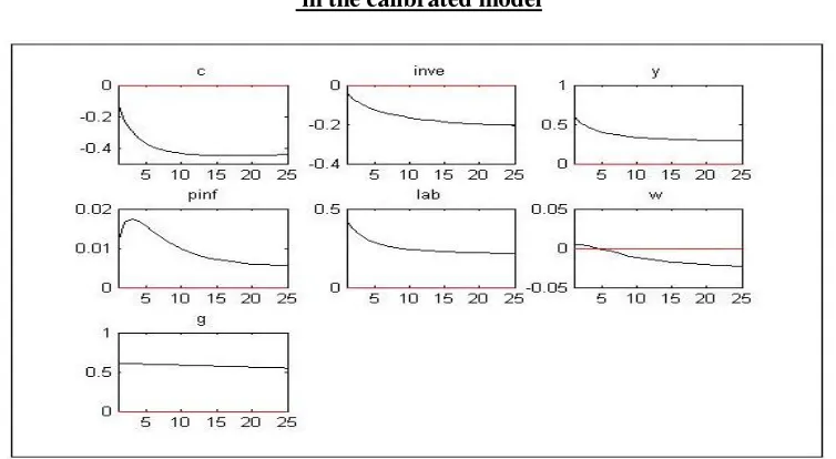
We start the analysis by conducting a stochastic simulation of the model. The following figure shows the responses of the variables of interest to a positive government spending shock in the calibrated model. The results show that following the shock, there is an immediate increase in output, wages, employment and inflation. Whereas, there is a decline in private consumption and investment.
Figure (1): The responses of the variables of interest to a positive government spending shock in the calibrated model
Source: the author’s results obtained from a calibrated model similar to SW, 2007.
9
[image:12.612.117.494.377.584.2]12
Regarding the model estimation, tables 3 to 5 (in the appendix) show the posterior means of the parameters and structural shocks together with 95% confidence intervals for the three model specifications covering the fiscal reforms period from 1997:Q4 to 2009:Q2.
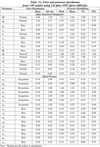
The posterior means of the price and wage mark-ups are high in (specification 2) compared to other versions of the model with 0.95 and 0.45, respectively. For the price and wage stickiness parameters the results indicate different values in the different models. DiCecio and Nelson (2007) suggest that price stickiness is higher compared to wage stickiness. We derive a different conclusion using specifications (1 and 3).10 On the other hand, the inclusion of fiscal policy rule in (specification 2) has reflected the role of price stickiness in deriving nominal rigidity.11 The results show that the partial indexation parameter of the wages is always lower than that for prices in the three models which is consistent with previous results using the UK data.
The posterior mean of the persistence parameter of government spending shock in the policy rule differs according to the model specification used in the analysis. Using the benchmark model, it was 0.26. The posterior mean of the ρg is equal to 0.5 using (specification 2). Whereas, it becomes 0.96 using (specification 3). This means that the observed shock in the policy rule is highly persistent compared to a moderate unobserved shock.
Regarding the standard deviation of the shocks
σ
g , the value is very high in the benchmark model and the 3rd specifications with values 1.52 and 2.32, respectively. However, using (specification 2) the standard deviation is 0.65. This result is consistent with the conclusion related to the persistence parameters shocks in the fiscal policy rule. This means that the 3rd specification is capturing the structural dynamics that are similar to the benchmark model. This is another advantage of including actual data in the analysis.Furthermore, the figures of the priors and the posterior densities are more convenient in the estimated period from 1997:Q4 to 2009:Q2 compared to the other samples. We claim that this result is appropriate to use for fiscal policy analysis and model comparison.
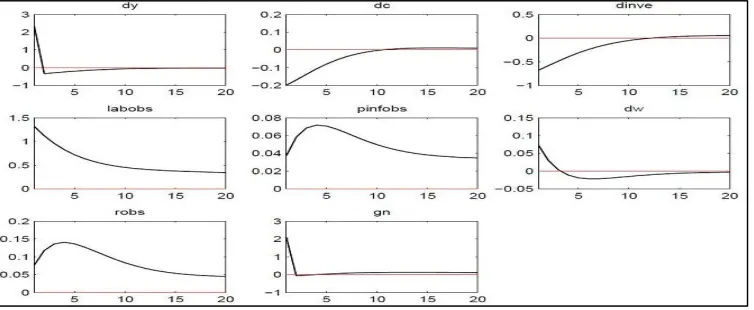
Interestingly, the analysis of fiscal policy shocks (in specification 3) indicates that following a positive government spending shock there is an immediate increase in output, inflation rate, nominal interest rate, worked hours and real wages. However, there is a decline in private consumption and private investment.
Another feature of the results is the reversed response of the above mentioned variable in the estimated model using the 2nd specification, as in figure 2. This suggests that the inclusion of government expenditure actual data guarantees obtaining similar immediate responses to the one resulting from the calibrated version, as in figure 1.
10
The posterior means of the Calvo parameters differs from that obtained by Faccini (2009) et al. and Harrison and Oomen (2010).
11
13
Figure (2): The responses of the variables of interest to a positive government spending shock using (specifications 2 and 3)
Source: the author’s result obtained from model estimation of (specification 2).
Source: the author’s result obtained from model estimation of (specification 3). Where (gn) is included to reflect the estimation of the feedback rule as in equation 14. The shock implies an observed shock which is derived from equation 14 that incorporates actual data for output and government spending.
The variance decomposition indicates that almost 64% of the variation in output is explained by the government spending shock. In addition, 21% of the variations in the worked hours and 13% of the variations in real wages are explained by the government spending shock. This indicates the relevance of the investigation of fiscal policy shocks in the model to labour market frictions.
[image:14.612.118.495.296.451.2]14
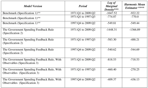
Table 2 investigates the model fit using different specifications and data samples. In general, the 3rd specification outperforms the other two models. The log of marginal data density and as the harmonic mean estimators are higher when the number of observations included are lowered.
[image:15.612.54.548.159.455.2]
Table 2: Reports marginal densities of different model versions*
Model Version Period
Log of Marginal Density***
Harmonic Mean Estimator ****
Benchmark (Specification 1)** 1971:Q1 to 2009:Q2 -1047.52 -922.22 Benchmark (Specification 1)** 1971:Q1 to 1997:Q3 -774.07 -770.0 Benchmark (Specification 1)** 1997:Q4 to 2009:Q2 -549.81 -549.44 The Government Spending Feedback Rule
(Specification 2)
1971:Q1 to 2009:Q2 -1448.31 -1366.89
The Government Spending Feedback Rule (Specification 2)
1971:Q1 to 1997:Q3 -583.30 -488.21
The Government Spending Feedback Rule (Specification 2)
1997:Q4 to 2009:Q2 -540.62 -544.69
The Government Spending Feedback Rule, With Observables (Specification 3)
1971:Q1 to 2009:Q2 -818.53 -718.53
The Government Spending Feedback Rule, With Observables (Specification 3)
1971:Q1 to 1997:Q3 -460.40 -270.25
The Government Spending Feedback Rule, With Observables (Specification 3)
1997:Q4 to 2009:Q2 -409.37 -436.13
Note: *Results are the author’s calculations.
**Our comparison takes the results in (SW, 2007) using UK data and the standard seven key macroeconomic variables as the benchmark.
***The marginal density has been calculated via the Laplace Approximation. Whereas, the initial value of the posterior mode is obtained using Chris Sim’s algorithm to maximize the likelihood function.
****The Harmonic mean estimator is obtained using the Metropolis-Hasting algorithm applied on Dynare.
This implies that for the policy analysis it is more relevant to divide the period under investigation into subsamples and compare the model fit. Moreover, in terms of the Bayes factor still the 3rd specification is desirable.
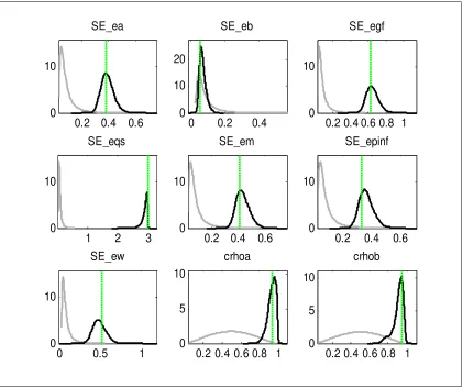
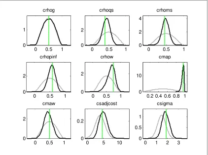
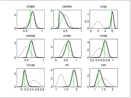
Figures 3 to 6 (in the appendix) show the prior, posterior distributions and the mode obtained with the maximisation of the posterior kernel using (specification 2). We see that the posterior distribution coincides with the mode derived from the MH samples, for some of the parameters. Also, we observe that the patterns of the prior and posterior distributions are too far from each other for some structural shocks. The later situation reflects that the observed data provide additional information for most parameters. 12
12
15
7.
Conclusion
The contribution of this paper is not only to estimate a medium scale (NKDSGE) model for the UK that is in line with (SW, 2007), and Christiano et al. (2005) using Bayesian methodology, but also the inclusion of a fiscal policy rule to investigate the possible structural changes due to the fiscal policy reforms in 1997.
The main results are the following. We establish that the inclusion of actual fiscal data in the fiscal policy rule enables the model to fit the data more closely. In addition, the inclusion of fiscal data for the period from 1997:Q4 to 2009:Q2 (the fiscal reform period) has an impact on the qualitative response of the main economic variables to the fiscal policy shock compared to a model estimated with the same fiscal rule but without actual fiscal data. We found that following a positive government spending shock (specification 3), there is an immediate increase in output, inflation rate, nominal interest rate, worked hours and real wages. However, there is a decline in private consumption and private investment.
Another feature of the results is the reversed response of the above mentioned variables in the estimated model using (specification 2). In addition, the government spending shock is moderate in (specification 2), whereas it is highly persistent in (specification 3) using the sample that covers the fiscal reform period.
Furthermore, the results are sensitive to the choice of priors, the number of Metropolis-Hasting (MH) replications, the scaling factor in the algorithm, the sample size, and the method of computation of the posterior mode.
16
References
• Adolfson, Malin , Laséen, Stefan , Lindé, Jesper , Villani, Mattias, (2007), Bayesian Estimation of an Open Economy DSGE Model with Incomplete Pass-Through, Journal of International Economics, Vol. 72(2), pp. 481-511, July.
• Adolfson, Malin , Laséen, Stefan , Lindé, Jesper , Villani, Mattias, (2005), Are Constant Interest Rate Forecasts Modest Interventions? Evidence from an Estimated Open Economy DSGE Model of the Euro Area, Working Paper Series No. 180, Sveriges Riksbank (Central Bank of Sweden).
• Afonso, António and Sousa M. Ricardo (2009), The Macroeconomic Effects of Fiscal Policy, The European Central Bank, working paper series No. 991, January.
• Aiyagari, S. Rao, and Christiano, Lawrence J. and Eichenbaum, Martin, (1992), The Output, Employment, and Interest Rate Effects Of Government Consumption, Journal of Monetary Economics, Vol. 30(1), pp. 73-86, October.
• Almeida, Vanda, (2009), Bayesian Estimation of a DSGE Model for the Portuguese Economy, Economic Research Department, Banco de Portugal, Working Papers No. 14, July.
• Botman, D., D. Muir, D. Laxton and A. Romanov (2006), A New-Open-Economy-Macro Model for Fiscal Policy Evaluation, IMF Working Paper 06/045.
• Burriel , Pablo and Fernandez-Villaverde, Jesus and Rubio-Ramirez, Juan F., (2009), MEDEA: a DSGE Model for the Spanish Economy, PIER Working Paper Archive 09-017, Penn Institute for Economic Research, Department of Economics, University of Pennsylvania.
• Calvo, G., A., (1983), Staggered Prices in a Utility-Maximising Framework, Journal of Monetary Economics, Vol. 12, pp. 383-98.
• Chari V. V., Kehoe, Patrick J. and Ellen R. McGrattan, (2009), New Keynesian Models: Not Yet Useful for Policy Analysis, American Economic Journal: Macroeconomics, American Economic Association, Vol. 1(1), pp. 242-66, January.
• Christiano, Lawrence, Martin Eichenbaum and Charlie Evans, (2005), Nominal Rigidities and the Dynamic Effects of a Shock to Monetary Policy, Journal of Political Economy, Vol. 113(1), pp. 1-45.
• Christopher J. Erceg , Luca Guerrieri , Christopher Gust, (2006), SIGMA: a New Open Economy Model for Policy Analysis, International Journal of Central Banking, Vol. 2(1), March.
• Dejong N., David and Dave, Cheatan, (2007), Structural Macroeconomics, Princeton University Press.
• Del Negro, M., F. Schorfheide, F. Smets, and R. Wouters (2007), On the Fit of New Keynesian Models, Journal of Business and Economic Statistics, Vol. 25(2), pp. 143-162.
• Del Negro, M., and F. Schorfheide (2004), Priors from General Equilibrium Models for VARs,
International Economic Review, 45(2), pp. 643-673.
• DiCecio, Riccardo and Nelson, Edward (2007), An Estimated DSGE Model for the United Kingdom, Research Division, Federal Reserve Bank of St. Louis, Working Paper Series, 2007-006A, February.
• Ellison, Martin and Scott, Andrew (2000), Sticky Prices and volatile output, Bank of England, Working Papers Series No. 127.
• Erceg, Christopher J., Henderson, Dale W., Levin, Andrew T., (2000), Optimal Monetary Policy With Staggered Wage and Price Contracts, Journal of Monetary Economics, Vol. 46(2), pp. 281-313, October.
• Faccini, Renato, Millard, Stephen and Zanetti, Francesco, (2009), Wage Rigidities in an Estimated DSGE Model of the UK Labour Market, The Bank of England’s research paper series.
17
• Garratt, Anthony, Lee, Kevin, Pesaran M. Hashem, Shin, Yongcheol, (2006), Global and National Macroeconometric Modelling: a Long-Run Structural Approach, Oxford University Press Inc., New York.
• Geweke, J. (1999), Using Simulation Methods for Bayesian Econometric Models: Inference, Development and Communication, Econometric Review, Vol. 18(1), pp. 1-126.
• Griffoli, Mancini, Tommaso (2009), An introduction to the solution and estimation of DSGE models, Dynare Version 4 - User Guide, November.
• Harrison, Richard, Kalin Nikolov, Meghan Quinn, Gareth Ramsay, Alasdair Scott, and Ryland Thomas, (2005), The Bank of England Quarterly Model, Bank of England Publications, London.
• Harrison, Richard and Oomen, Özlem, (2010), Evaluating and estimating a DSGE model for the United Kingdom,The Bank of England’s working paper series, Working Paper No. 380.
• Jesús Fernández-Villaverde, (2009), The Econometrics of DSGE Models, NBER Working Paper
No. 14677, January.
• Kamal, Mona (2010), Empirical Investigation of Fiscal Policy Shocks in the UK,
Empirical
Economic Letters
, Vol. 9(4), April.
• Kim, K. and A. R. Pagan (1995), The Econometric Analysis of Calibrated Macroeconomic Models, Chapter 7 in M. H. Pesaran and M. Wickens (eds.), Handbook of Applied Econometrics: Macroeconomics. Basil Blackwell: Oxford
• Kydland, F. E. and Prescott, E. C. (1982), Time to build and aggregate fluctuations,
Econometrica, vol. 50(6), November, pp. 1345-70.
• Lubik, Thomas and Schorfheide, Frank (2005), A Bayesian Look at New Open Economy Macroeconomics, Chapter in NBER book, NBER Macroeconomics Annual 2005, Vol. 20, editors: Mark Gertler and Kenneth Rogoff, pp. 313-382, April.
•Lubik and Schorfheide (2007), Do central banks respond to exchange rate movements? A structural investigation, Journal of Monetary Economics, Vol. 54, pp. 1069-1087.
•Monacelli, Tommaso and Perotti, Roberto (2006), Fiscal policy, the Trade Balance and the Real Exchange Rate: Implications for International Risk Sharing, IGIER (Innocenzo Gasparini Institute for Economic Research), Bocconi University, June.
•Mountford, Andrew and Uhlig, Harald (2009), What Are the Effects of Fiscal Policy Shocks?,
Journal of Applied Econometrics, Vol. 24(6), pp. 960-992, September .
• Pytlarczyk , Ernest (2005),An Estimated DSGE Model for the German Economy within the Euro Area, Deutsche Bundesbank, Discussion Paper Series, No. 33/2005.
• Ravn, Morten, Schmitt-Grohe, Stephanie, Uribe, Martin (2007), Explaining the Effects of Government Spending Shocks on Consumption and the Real Exchange Rate, National Bureau of Economic Research, Working Paper No. 13328, August.
• Ravenna, F. (2007), Vector Autoregression and Reduced Form Representations of DSGE Models,
Journal of Monetary Economics, Vol. 54(7), pp. 2048-2064.
• Ruge-Murcia, F. J. (2007), Methods to Estimate Dynamic Stochastic General Equilibrium Models, Journal of Economic Dynamics and Control, Vol. 31, pp. 2599-2636.
• Schmitt-Groh´e, S. and M. Uribe (2000), Price Level Determinacy and Monetary Policy under a Balanced-Budget Requirement, Journal of Monetary Economics, Vol. 45, pp. 211-246.
• Schmitt-Groh´e, S. and M. Uribe (2004), Optimal Simple and Implementable Monetary and Fiscal Rules, Journal of Monetary Economics, Vol.54, pp. 1702-1725.
• Smets, Frank and Raf Wouters (2003), An Estimated Dynamic Stochastic General Equilibrium Model of the Euro Area, Journal of the European Economic Association, September, Vol. 1(5), pp. 1123-1175.
18
Appendix: Data Description and Sources
The data in this paper spans from 1971:Q1 to 2009:Q2 for the UK. We have used three data sources. The Office for National Statistics (ONS) in the UK, the Main Economic Indicators (MIE) provided by the website of the Organization of Economic Cooperation and Development (OECD), and the International Financial Statistics (IFS) published by the International Monetary Fund (IMF).
• Gross Domestic Product (GDP): quarterly data, seasonally adjusted from the data source (ONS).
• GDP Deflator: quarterly data, seasonally adjusted from the data source, the Office for National Statistics (ONS).
• Wages: quarterly data, seasonally adjusted from the data source, the OECD, Main economic Indicators (MIE). Wages are defined as the index (2005=100) of hourly earnings in manufacturing.
• Private Consumption: quarterly data, seasonally adjusted from the data source (ONS).
• Government Spending: following the relevant empirical literature, the government spending variable is defined as total purchases of goods and services (i.e. government consumption plus government investment). The source is (ONS). The data is seasonally adjusted using (TRAMO-SEATS method).
• Private Investment: quarterly data, seasonally adjusted from the data source (ONS).
• Government Revenues: defined as total tax revenues minus transfers (including interest payments). The source is (ONS). The data are seasonally adjusted using (TRAMO-SEATS method).
19
Table (3): Prior and posterior distribution
from (SW model) using UK data (1997:Q4 to 2009:Q2)
Parameter Prior Distribution Posterior Distribution Mean Std. dev. Mode Mean 5% 95%
Main Structural Parameters
ϕ
Normal 4.00 1.50 4.2 3.86 2.00 5.42c
σ
Normal 1.50 0.37 0.47 0.52 0.28 0.79h
Beta 0.70 0.10 0.83 0.84 0.77 0.90w
ζ Beta 0.50 0.10 0.63 0.63 0.54 0.72
l
σ Normal 2.00 0.75 2.7 2.28 0.92 3.54 p
ζ
Beta 0.50 0.10 0.62 0.61 0.50 0.70w
ι Beta 0.50 0.15 0.38 0.42 0.22 0.61
p
ι Beta 0.50 0.15 0.63 0.61 0.45 0.78
ψ
Beta 0.50 0.15 0.33 0.32 0.12 0.51Φ Normal 1.25 0.12 1.66 1.67 1.50 1.84
π
r
Normal 1.50 0.25 1.25 1.20 1.00 1.37ρ
Beta 0.75 0.10 0.59 0.62 0.52 0.72y
r Normal 0.12 0.05 0.18 0.20 0.13 0.27 y
r∆ Normal 0.12 0.05 0.16 0.16 0.08 0.25 α Normal 0.30 0.05 0.23 0.24 0.15 0.31
Shock Process
a
σ Invgamma 0.10 2.00 0.41 0.42 0.34 0.51
b
σ
Invgamma 0.10 2.00 0.07 0.08 0.05 0.11g
σ Invgamma 0.10 2.00 1.46 1.52 1.26 1.78
I
σ Invgamma 0.10 2.00 3.00 2.90 2.75 3.00
r
σ Invgamma 0.10 2.00 0.38 0.41 0.33 0.49
p
σ
Invgamma 0.10 2.00 0.08 0.11 0.05 0.17w
σ Invgamma 0.10 2.00 0.28 0.29 0.19 0.40
a
ρ Beta 0.50 0.20 0.95 0.93 0.88 0.99
b
ρ Beta 0.50 0.20 0.93 0.92 0.88 0.96
g
ρ Beta 0.50 0.20 0.23 0.26 0.08 0.43
I
ρ Beta 0.50 0.20 0.35 0.44 0.27 0.60
r
ρ
Beta 0.50 0.20 0.39 0.41 0.26 0.57p
ρ Beta 0.50 0.20 0.90 0.85 0.73 0.97
w
ρ Beta 0.50 0.20 0.50 0.56 0.32 0.80
p
µ Beta 0.50 0.20 0.23 0.24 0.04 0.43
w
µ Beta 0.50 0.20 0.34 0.34 0.09 0.57 Note: *Results are the author’s calculations.
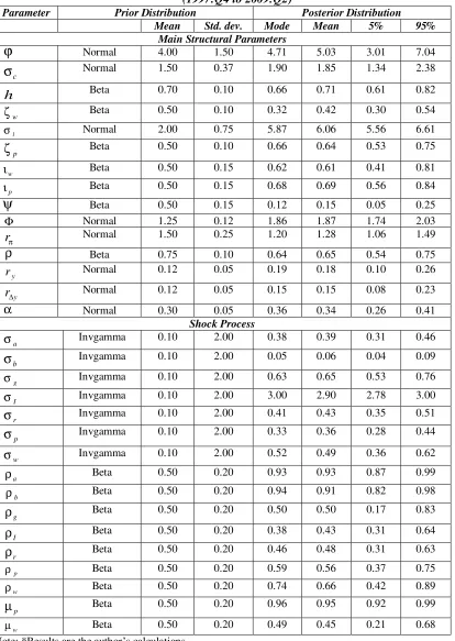
[image:20.612.84.503.70.683.2]20
Table (4):
Prior and posterior distribution from (the general feedback rule specification without observable) using UK data (specification 2)(1997:Q4 to 2009:Q2)
Parameter Prior Distribution Posterior Distribution Mean Std. dev. Mode Mean 5% 95%
Main Structural Parameters
ϕ
Normal 4.00 1.50 4.71 5.03 3.01 7.04c
σ
Normal 1.50 0.37 1.90 1.85 1.34 2.38h
Beta 0.70 0.10 0.66 0.71 0.61 0.82w
ζ Beta 0.50 0.10 0.32 0.42 0.30 0.54
l
σ Normal 2.00 0.75 5.87 6.06 5.56 6.61
p
ζ
Beta 0.50 0.10 0.66 0.64 0.53 0.75w
ι Beta 0.50 0.15 0.62 0.61 0.41 0.81
p
ι Beta 0.50 0.15 0.68 0.69 0.56 0.84
ψ
Beta 0.50 0.15 0.12 0.15 0.05 0.25Φ Normal 1.25 0.12 1.86 1.87 1.74 2.03
π
r
Normal 1.50 0.25 1.20 1.28 1.06 1.49ρ
Beta 0.75 0.10 0.64 0.65 0.54 0.75y
r Normal 0.12 0.05 0.19 0.18 0.10 0.26 y
r∆ Normal 0.12 0.05 0.15 0.15 0.08 0.23 α Normal 0.30 0.05 0.36 0.34 0.26 0.41
Shock Process
a
σ Invgamma 0.10 2.00 0.38 0.39 0.31 0.46
b
σ
Invgamma 0.10 2.00 0.05 0.06 0.04 0.09g
σ Invgamma 0.10 2.00 0.63 0.65 0.53 0.76
I
σ Invgamma 0.10 2.00 3.00 2.90 2.78 3.00
r
σ Invgamma 0.10 2.00 0.41 0.43 0.35 0.51
p
σ
Invgamma 0.10 2.00 0.33 0.36 0.28 0.44w
σ Invgamma 0.10 2.00 0.52 0.49 0.36 0.62
a
ρ Beta 0.50 0.20 0.93 0.93 0.87 0.99
b
ρ Beta 0.50 0.20 0.94 0.91 0.82 0.98
g
ρ Beta 0.50 0.20 0.50 0.50 0.17 0.83
I
ρ Beta 0.50 0.20 0.38 0.43 0.31 0.64
r
ρ
Beta 0.50 0.20 0.46 0.48 0.31 0.63p
ρ Beta 0.50 0.20 0.59 0.56 0.37 0.75
w
ρ Beta 0.50 0.20 0.74 0.66 0.42 0.89
p
µ Beta 0.50 0.20 0.96 0.95 0.92 0.99
w
µ Beta 0.50 0.20 0.49 0.45 0.21 0.68 Note: *Results are the author’s calculations.
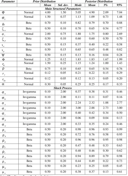
[image:21.612.90.504.106.689.2]21
Table (5):
Prior and posterior distribution
from (the general feedback rule specification with observable) using UK data (specification 3) (1997:Q4 to 2009:Q2)
Parameter Prior Distribution Posterior Distribution Mean Std. dev. Mode Mean 5% 95%
Main Structural Parameters
ϕ
Normal 4.00 1.50 5.05 4.90 2.09 7.04c
σ
Normal 1.50 0.37 1.13 1.09 0.73 1.48h
Beta 0.70 0.10 0.82 0.79 0.70 0.88w
ζ Beta 0.50 0.10 0.70 0.65 0.54 0.77
l
σ Normal 2.00 0.75 1.88 1.75 0.80 2.69
p
ζ
Beta 0.50 0.10 0.60 0.60 0.50 0.70w
ι Beta 0.50 0.15 0.37 0.40 0.22 0.58
p
ι Beta 0.50 0.15 0.65 0.65 0.48 0.82
ψ
Beta 0.50 0.15 0.13 0.16 0.04 0.28Φ Normal 1.25 0.12 1.83 1.83 1.67 1.99
π
r
Normal 1.50 0.25 1.15 1.24 1.00 1.43ρ
Beta 0.75 0.10 0.65 0.65 0.54 0.76y
r Normal 0.12 0.05 0.21 0.22 0.15 0.29 y
r∆ Normal 0.12 0.05 0.12 0.13 0.05 0.20 α Normal 0.30 0.05 0.25 0.25 0.17 0.33
Shock Process
a
σ Invgamma 0.10 2.00 0.37 0.38 0.31 0.46
b
σ
Invgamma 0.10 2.00 0.11 0.11 0.07 0.16g
σ Invgamma 0.10 2.00 2.24 2.32 1.88 2.77
I
σ Invgamma 0.10 2.00 3.00 2.88 2.73 3.00
r
σ Invgamma 0.10 2.00 0.40 0.42 0.34 0.50
p
σ
Invgamma 0.10 2.00 0.06 0.09 0.04 0.13w
σ Invgamma 0.10 2.00 0.33 0.35 0.24 0.46
a
ρ Beta 0.50 0.20 0.98 0.96 0.93 0.99
b
ρ Beta 0.50 0.20 0.72 0.76 0.58 0.95
g
ρ Beta 0.50 0.20 0.96 0.96 0.95 0.98
I
ρ Beta 0.50 0.20 0.47 0.48 0.33 0.63
r
ρ
Beta 0.50 0.20 0.48 0.46 0.30 0.62p
ρ Beta 0.50 0.20 0.94 0.89 0.79 0.98
w
ρ Beta 0.50 0.20 0.44 0.49 0.22 0.73
p
µ Beta 0.50 0.20 0.23 0.25 0.05 0.45
w
µ Beta 0.50 0.20 0.38 0.37 0.13 0.61 Note: *Results are the author’s calculations.
[image:22.612.87.505.113.688.2]22
Figure (3):
The prior, posterior distributions and the mode obtained with the maximization of
the posterior kernel using (specification 2)
0.2 0.4 0.6
0 10
SE_ea
0 0.2 0.4
0 10 20
SE_eb
0.2 0.4 0.6 0.8 1 0
10
SE_egf
1 2 3
0 10
SE_eqs
0.2 0.4 0.6
0 10
SE_em
0.2 0.4 0.6
0 10
SE_epinf
0 0.5 1
0 10
SE_ew
0.2 0.4 0.6 0.8 1 0
5 10
crhoa
0.2 0.4 0.6 0.8 1 0
5 10
crhob
[image:23.612.97.517.111.464.2]23
Figure (4): The prior, posterior distributions and the mode obtained with the maximization of
the posterior kernel using (specification 2)
0 0.5 1
0 1
crhog
0 0.5 1
0 2
crhoqs
0 0.5 1
0 2 4
crhoms
0 0.5 1
0 2
crhopinf
0 0.5 1
0 2
crhow
0.2 0.4 0.6 0.8 1 0
10
cmap
0 0.5 1
0 2
cmaw
0 5 10
0 0.2
csadjcost
0 1 2 3
0 0.5 1
csigma
[image:24.612.96.518.139.453.2]24
Figure (5): The prior, posterior distributions and the mode obtained with the maximization of
the posterior kernel using (specification 2)
0.5 1
0 5
chabb
0.5 1
0 5
cprobw
0 2 4 6
0 0.5 1
csigl
0.5 1
0 5
cprobp
0 0.5 1
0 2
cindw
0.2 0.4 0.6 0.8 1 0
2 4
cindp
0 0.2 0.4 0.6 0.8 0
5
czcap
1 1.5 2
0 2 4
cfc
1 1.5 2
0 2
crpi
[image:25.612.96.519.113.430.2]25
Figure (6): The prior, posterior distributions and the mode obtained with the maximization of
the posterior kernel using (specification 2)
0.4 0.6 0.8
0 5
crr
0 0.2 0.4
0 5
cry
0 0.2 0.4
0 5
crdy
0.20.40.60.8 1 1.2 0
2 4
constepinf
0 0.5 1
0 2 4
constebeta
-10 -5 0 5
0 0.5 1
constelab
0 0.2 0.4 0.6
0 5
ctrend
0 1 2
0 1
cgy
0.2 0.4 0.6
0 5
calfa
[image:26.612.97.517.110.429.2]