On the epidemic of financial crises

Munich Personal RePEc Archive

On the epidemic of financial crises

Demiris, Nikolaos and Kypraios, Theodore and Smith, L.

Vanessa

Athens University of Economics and Business, University of

Nottingham, University of Cambridge

November 2012

On the Epidemic of Financial Crises

Nikolaos Demiris

Theodore Kypraios

L. Vanessa Smith

Athens University of University of Nottingham University of Cambridge

Economics & Business

November 2012

Abstract

This paper proposes a framework for modelling …nancial contagion that is based on SIR (Susceptible-Infected-Recovered) transmission models from epidemic theory. This class of models addresses two important features of contagion modelling, which are a common shortcoming of most existing empirical approaches, namely the direct mod-elling of the inherent dependencies involved in the transmission mechanism, and an associated canonical measure of crisis severity. The proposed methodology naturally implies a control mechanism, which is required when evaluating prospective immunisa-tion policies that intend to mitigate the impact of a crisis. It can be implemented not only as a way of learning from past experiences, but also at the onset of a contagious …nancial crisis. The approach is illustrated on a number of currency crisis episodes, using both historical …nal outcome and temporal data. The latter require the intro-duction of a novel hierarchical model that we call the Hidden Epidemic Model (HEM), and which embeds the stochastic …nancial epidemic as a latent process. The empirical results suggest, among others, an increasing trend for global transmission of currency crises over time.

Keywords: Financial crisis, contagion, stochastic epidemic model, random graph, MCMC

JEL Classi…cation: C51, G01, C15, G15, C11.

1

Introduction

A …nancial crisis originating in one country can travel within and beyond its original

neigh-bourhood spreading among countries like a contagious disease. Loosely speaking, this

phe-nomenon, which was a common feature of the major recent crises, is referred to by economists

as ‘contagion’. Contagion by de…nition can only occur if there are interactions among

sub-jects. These interactions can materialise at di¤erent levels and through di¤erent channels

simultaneously, some channels being more important during particular events than

oth-ers.1_{As …nancial crises spread across countries, they a¤ect nations with apparently healthy}

fundamentals and sound policies. The better understanding we have of their propagation

mechanism, the better we are positioned in proposing policy interventions which can most

e¤ectively reduce their contagious spread.

The economics and …nance literature have a number of theoretical models that aim

to explain the contagious spread of crises, emphasising trade linkages (bilateral or third

party, Gerlach and Smets, 1995; Corsetti et al., 1998), …nancial linkages (Allen and Gale,

2000), as well as models on information asymmetries and investor behaviour (Calvo and

Mendoza, 2000; Kodres and Pritsker, 2002), among others. More recently, recognition of the

inherent complexities and interconnections associated with …nancial systems has advocated

the need to consider methods from other disciplines such as ecology, epidemiology, biology

and engineering in studying …nancial networks (May et al. 2008, Haldane, 2009). Indeed,

researchers have turned to alternative methods in modelling …nancial contagion, which are

largely based on numerical simulations. For example, Gai and Kapadia (2010) study a

percolation-type process on a weighted network of banks as a model of contagion.2_{They make}

use of tools from contemporary network theory, which have lately been gaining considerable

popularity. May and Arinaminpathy (2010) pursue recent advances in the area of complex

ecological systems in a study similar in spirit to Gai and Kapadia, though they employ a

mean …eld approximation rather than resorting to simulations. Amini et al. (2010) analyse

distress propagation in a network of banks, via a cascading process, and derive the asymptotic

1_{The literature typically distinguishes between fundamentals-based contagion, a transmission of a crisis} from one country to another through real and …nancial linkages, also known as spillovers, and pure contagion where a crisis might trigger additional crises elsewhere for reasons unexplained by fundamentals.

magnitude of contagion. Caporale et al. (2009) make use of agent-based simulation models

to investigate the dynamics of …nancial contagion.

On the empirical front considerable e¤ort has been devoted to documenting the existence

of contagion.3 _{The bulk of the studies suggest that there is evidence of contagion. For an}

overview of the empirical evidence of contagion see Dornbusch et al. (2000) and Pericoli

and Sbracia (2003). Less emphasis, however, has been placed on modelling the propagation

mechanism of …nancial crises. A class of models that features prominently in the empirical

contagion literature is that of cross country probit-type regressions of a binary crisis indicator

on variables representing potentially important transmission channels. Such channels have

been identi…ed as trade links, Glick and Rose (1999), …nancial links and the common creditor,

Caramazza et al. (2004) and Kaminsky and Reinhart (2000), neighborhood e¤ects, De

Gregorio and Valdes (2001), and macroeconomic similarities, Sachs et al. (1996). More

recently, Dungey and Martin (2007) have proposed capturing …nancial market linkages during

crises through the use of common factors, while Aït-Sahalia et al. (2010) suggest modelling

…nancial contagion using mutually exciting processes.

In this paper we propose a framework for modelling …nancial contagion which is based

on SIR (Susceptible-Infected-Recovered) transmission models from epidemic theory (see for

example, Bailey, 1975). This class of models addresses two important features of contagion

modelling which are a common shortcoming of most existing empirical approaches, namely

the direct modelling of the inherent dependencies involved in the transmission mechanism,

and an associated canonical measure of crisis severity. At the same time, it allows to

in-corporate features that re‡ect relevant theoretical and empirical evidence in the literature

through the inclusion of appropriate covariates. The proposed methodology naturally implies

a control mechanism, which is required when evaluating prospective immunisation policies

that intend to mitigate the impact of a crisis. This control mechanism can be implemented

not only as a way of learning from past experiences, but also in real-time as a contagious

…nancial crisis unfolds.

Speci…cally, the approach is based on a stochastic epidemic transmission process where

the population of countries is explicitly structured, and a crisis may be propagated both

locally and globally. Having identi…ed all countries that su¤ered during a particular crisis

episode, the focus is on how crises spread from an initially a¤ected (or ‘infected’) country

to the rest of the countries by considering their interaction at the local and global level.

We explicitly model regional and global contagious ‘contacts’ and infer the rate of their

transmission. These transmission rates allow us to directly quantify the severity of the

crisis, in contrast to conventional approaches in the literature where severity is measured

by a composite index of macroeconomic indicators, see Kaminsky and Reinhart (1998) and

Kaminsky (2006). The methodology also delivers an estimate of the number of countries to

provide …nancial support to, in order to prevent a major crisis.

In the proposed framework a country may experience a crisis not only because of its

direct links to the originally infected (ground zero) country, but also due to local and/or

global contacts with countries that are already infected. Thus, we allow for the so called

‘cascading e¤ect’ following the terminology of Glick and Rose (1999), which is typically

ignored in the literature. In fact, the proposed approach e¤ectively considers the set of all

possible transmission channels of a crisis. Furthermore, it naturally accounts for an increase

in the likelihood of a crisis in a particular country given that there is a crisis elsewhere.

This is explored in Eichengreen et al. (1996) and Kaminsky and Reinhart (2000) as being

consistent with the existence of contagion.

The methodology is illustrated on a number of currency crisis episodes, using both

his-torical …nal outcome and temporal data. The former provides information on the number

of initially ‘healthy’ countries, that were ever a¤ected or otherwise by a particular …nancial

crisis. The information provided by the latter allows to estimate the ‘infection’ and/or

‘re-covery’ times of the crisis, in addition to the trasmission rates. The use of temporal data

is necessary for performing real-time analysis of a crisis spread. It requires the introduction

of a novel hierarchical model, that we call the Hidden Epidemic Model (HEM), and which

embeds the stochastic …nancial epidemic as a latent process. Our …ndings, among others,

point to an increasing trend for global transmission of currency crises over time.

The paper is structured as follows. In Section 2 we introduce the modelling framework and

describe the inference procedure associated with …nal outcome data. Section 3 describes the

hidden epidemic model associated with the use of temporal data. In Section 4 the proposed

5 discusses the relevance of the methodology for policy analysis. Section 6 contains some

further discussion.

2

Modelling Framework

Consider the onset of a …nancial crisis, for example, a currency crisis or a stock market

crash, with contagious e¤ects to a given population of, say, countries.4 _{Our interest is in}

modelling the process associated with the propagation of the crisis. The approach can be

equally applied to populations of …rms or banks, among others.

2.1

The Model

Consider a closed population of N countries, partitioned into regions of varying sizes.

Speci…cally we will assume that the population contains rj regions/groups of size j, where

r=PS_j=1rj is the total number of regions and S denotes the size of the largest group. The

total number of countries is then N = PS_j=1jrj. The crisis originates in a typically small

number of countries. At the outset, all countries are deemed susceptible to the particular

crisis episode. As the crisis unfolds, each country is considered to belong to any one of

three states: susceptible, infected (and ‘infectious’) or recovered. Such processes are often

referred to as SIR models in epidemic theory. In the SIR model a susceptible country is in

a ‘normal’ state and can be a¤ected by the crisis in question. An infective country is in a

state of crisis and may trasmit it to other countries. At the end of its infectious period an

individual country is considered recovered, in the sense that it plays no further role in the

propagation of the crisis. Thus, we e¤ectively assume that a country may not experience

multiple recoveries within a single crisis, which appears reasonable for such applications.

A country, say j, remains in crisis for a positive random time, denoted by Ij, which is

allowed to follow any speci…ed distribution. The periods for which the individual countries

remain in crisis are assumed to be a-priori independent. While infectious, a country may

transmit the crisis to each country within its region at times given by the points of a Poisson

process of rate L. Additionally, each country may trasmit the crisis to any given country

worldwide according to a Poisson process with rate G=N. That is, there are two levels

of mixing between countries, namely at the local and global level. The contact processes

within this construction are assumed to be a-priori independent. This formulation of the

model e¤ectively assumes that each country has local contacts with rate L+ G=N.

Al-ternative parameterisations of the epidemic model can be obtained using the superposition

and splitting of the Poisson process (see Kingman, 1993). The crisis ends when there are

no remaining infectious countries in the population. Notice the di¤erent scaling of the two

transmission rates. This is a common assumption in two-level-mixing models and it implies

that there will be more infectious contacts locally if the local population grows, while this is

not the case globally.

The model described above is a stochastic epidemic two level mixing model introduced

in Ball et al. (1997), where a detailed discussion of related work can be found. While the

model does not explicitly assume a latent period for the crisis to unfold once a particular

country has been a¤ected, but rather assumes immediate infection, the distribution of the

…nal outcome is invariant to very general assumptions concerning a latent period (see Ball

et al., 1997; Andersson and Britton, 2000). The two level mixing model encompasses the so

called generalised stochastic epidemic model (GSE), which arises by setting ( L= 0; G= ),

that is, assuming all countries mix homogeneously with rate :5

Epidemic models in their simple deterministic form are not foreign to the economics

lit-erature. They typically feature in studies of treatment and control, see for example Geo¤ard

and Philipson (1997), Gersovitz and Hammer (2004) and Toxvaerdy (2010). However, for a

complex, highly non-linear phenomenon such as contagion, the stochastic model described

above is more appropriate compared to any simple deterministic analog. It is particularly

ad-vantageous in that it is suitable for small populations, it can account for the regional/global

nature of a crisis, while model complexity and realism can be naturally expanded in di¤erent

directions, some of which will be discussed below.

Figure 1 illustrates a potential con…guration of a crisis spread in the case of a small

population of …ve countries denoted by {1,2,...,5}. The …ve countries are partitioned into

two regions, represented by the two circles. Consider 1 as the country originally a¤ected by

the crisis in question. The grey links denote contacts made locally between countries within

a region. The black links correspond to global contacts. The solid directed links represent

contacts that, resulted in infection, while the dashed links represent lack of contact in both

directions. Thus, in this particular con…guration the crisis is transmitted from country 1 to

countries 2 and 4.

Figure 1: Example of a crisis spead over a small population of countries

In the speci…cation described above the population of countries is assumed to represent a

complete network i.e. any country can have contacts with any other locally and globally. This

is not a restrictive assumption as epidemics upon random networks can be reparameterised to

correspond to epidemics on complete graphs (e.g. Neal, 2006, Newman, 2010), and thus can

be incorporated into the proposed framework. Furthermore, the population is assumed to

be homogeneous, that is, all countries posses similar infectivity and susceptibility properties.

This assumption will be relaxed in Section 4.1.1.

Further detail can be added to the model by dissagregating the population according to

individual attributes and/or relationship networks based, for example, on economic

informa-tion. These details can be incorporated through the transmission rates leading to weighted

networks. The study of a dynamic process on a weighted network is, essentially, equivalent

to the inclusion of a covariate. This can be easily seen by considering the moment

gener-ating function of the transmission rate, say ( ), where ( ) = E(exp( I)). In the case of a constant infectious period this is simply exp( I), the probability of avoiding infec-tion. When information about a particular variable, say X, becomes available, this can

be incorporated using a Cox-type (log-linear) model: = 0exp( X): Then ( ) becomes

( ) = exp[ I 0exp( X)] = wexp( 0I) = w ( 0). In other words, the inclusion of

more than one variable) is straightforward as will be illustrated in Section 4.2.2. If the focus

is, for example, on the contagious default of banks these covariates could represent balance

sheet information and/or information on interbank relations. In the case of a currency crisis,

they could represent trade and …nancial linkages between countries. Additional covariates

accounting for macroeconomic conditions could also be included.

2.2

Threshold Parameter

An appealing feature of the proposed modelling framework is that it embodies a threshold

parameter which can be utilised as a severity measure of the crisis, thus providing an inherent

control mechanism. Stochastic models such as epidemic and branching processes typically

generate bimodal realisations where an epidemic may or may not die out quickly, depending

on the value of the threshold parameter R0, often referred to as the basic reproduction

number. This is the most important parameter in epidemic theory (Dietz, 1993) and it is

de…ned as the expected number of infections generated by a typical infective in an in…nite

susceptible population. Generally, R0 is calculated as the largest eigenvalue of the so called

next generation matrix (Diekmann and Heesterbeek, 2000).

In the case of a homogeneously mixing stochastic epidemic, it holds that R0 = E(I);

where is the contact rate and I is the infectious period. R0 may be interpreted as a

threshold parameter since its value determines whether or not a major crisis can occur. In

particular, if R0 >1 a positive proportion of the in…nite population will be a¤ected by the

crisis with positive probability, while if R0 1 only a …nite number of susceptibles will ever

become infected and thus the crisis spread will swiftly die out. Hence, most control measures

aim to reduceR0 below unity. Ball and Donelly (1995) rigorously established the threshold

behaviour of the general stochastic epidemic by coupling the early stages of the epidemic

with a suitable branching process.

For the two-level mixing model the threshold parameter, denoted by R ; is de…ned in a

similar way to R0. In this case, Ball et al. (1997) couple the epidemic with a branching

process de…ned on groups. They show that

where v( L)is the average group …nal size if only local infections are permitted. Speci…cally,

v( L) = 1_gPS_j=1j j j; where j is the …nal size within a group of size j, j = rj=r is the

proportion of groups of sizej andg is the mean group size. It should be noted that whileR

is linear in G, it is nonlinear in L but linear in v( L), with the latter being an increasing

function of L: Details of the calculation of v( L) can be found in the appendix.

Most statistical analyses require the assumption of supercriticality, that is R > 1 so that a major crisis spread is possible (e.g. Rida, 1991; Demiris and O’Neill, 2005b). Since

prophylactic measures aim to achieve R 1, assuming that R > 1 is not desirable, as it also results in underestimating the variability of the model parameters. The inference

procedure we will employ does not condition upon R >1.

2.3

Inference Using Final Outcome Data

2.3.1 Final Size Distribution

For a given crisis episode, when only information on the …nal infected number of countries is

available, i.e. …nal outcome data, it is in principle possible to write down a system of recursive

linear equations, the solution of which delivers the probability mass function required for the

likelihood. However, solving such a set of equations can be numerically unstable even for

small population sizes (see for example Andersson and Britton, 2000, p.18). This problem

is greatly ampli…ed for more complex cases like the two level mixing model considered here.

The remainder of this section is concerned with the description of an inference procedure

that surmounts this complication.

2.3.2 Data and Likelihood

For the two level mixing model, the data are of the form x _{= fxijg where xij denotes the} number of regions containing j initially susceptible countries of which i ever su¤ered the

crisis in question. We will describe a Bayesian inference procedure for the two infection

rates L and G, givenx. By Bayes’ Theorem, the posterior density, ( L; G jx), satis…es

( L; G j x)/ (xj L; G) ( L; G); where (xj L; G) denotes the likelihood function

and ( L; G) the joint prior of ( L; G). The numerical problems mentioned in Section

very small number of countries. We surpass this di¢culty by following Demiris and O’Neill

(2005a) in augmenting the parameter space using an appropriate random directed graph

(digraph) as considered below.6

2.3.3 Random Digraph

The characterisation of the …nal outcome of a stochastic epidemic in terms of random graphs

is well known in epidemic theory and has been exploited by Ludwig (1975) and Barbour

and Mollison (1990) among others. It has been considered for the purposes of statistical

inference by Demiris and O’Neill (2005a); see also O’Neill (2009). In short, let each country

correspond to a vertex in the random digraph, while a directed edge in the graph denotes

a potential infection. The edges are drawn from vertex j with probability 1 exp( Ij L)

(1 exp( Ij G=N)) for local (global) links. It then holds that the distribution of the …nal

outcome of the crisis is equivalent to the distribution of the ‘giant component’ of the graph,

that is, the random set of vertices that are connected to the initially a¤ected country (or

countries) through directed edges. Notice that additional edges may exist in the digraph, but

only the routes emanating from the initially infected can correspond to actual ‘infections’.

Moreover, ‡exible models for the infectious periodsIj such as disjoint intervals in real time,

representing for example stock market opening times in the case of a stock market crash, can

be easily incorporated into this framework as they only appear through the edge probabilities.

To maximise computational e¢ciency we only consider the graph on ‘infected’ vertices, while

all other data contributions are accounted for via the likelihood.

2.3.4 Augmented Likelihood and Posterior

Suppose that the total number of countries that are ever a¤ected by a particular crisis is

n=P_iP_jixij, labeled1; : : : ; n, and de…neGas the random digraph on thesenvertices. For

j = 1; : : : ; nletIj denote the infectious period corresponding to vertexjandI = (I1; : : : ; In).

We assume that initially there is one known country in crisis, although it is trivial to consider

any number of initial infectives, possibly of unknown identity. In fact, it turns out that

knowledge of the initial infective is not crucial in the applications to follow.

The augmented posterior density may be written as

( L; G;I; Gjx)/ (xj L; G;I; G) (Gj L; G;I) (I) ( L; G): (2)

In (2), ( L; G) and (I) denote the priors while the …rst two terms e¤ectively represent

the augmented likelihood, given by L(x _{j L; G;}I_{; G). Provided that G is compatible}

with the data, L(x _{j L; G;}I_{; G) is evaluated as the probability of the edges in G times}

the probability of no edges between the n vertices in G and the remaining N n vertices.

Otherwise, L(x_{j L; G;}I_{; G)is set to zero.}

Let`L

j (`Gj ) denote the number of local (global) links emanating from vertexj andNjLthe

number of countries inj’s region. Further, let G x_{denote the event thatG is compatible}

with the data. Then the augmented likelihood can be written as

L(x_{j L; G;}I_{; G) := (}x_{j L; G;}I_{; G) (Gj L; G;}I_{) =}1_{G x}

n Y

j=1

h

f1 exp ( LIj)g`

L j

exp LIj NjL `Lj 1 exp

GIj

N

`G j

exp GIj(N `

G j )

N

!#

; (3)

where 1_{C denotes the indicator function which takes the value of one when the event C}

materialises, and zero otherwise. The MCMC algorithm used to sample from (2) is largely

similar to that in Demiris and O’Neill (2005a) where additional details can be found. In

brief, standard random walk Metropolis samplers are su¢cient for updating the infection

rates, while updating G requires some attention. Speci…cally, Gis a discrete random object

with an enormous number of possible con…gurations, the overwhelming majority of which

have negligible posterior probability. Hence, simple strategies like adding and deleting one

edge at a time are preferable, as samplers based on more complex proposals can exhibit poor

3

A Hidden Epidemic Model

Thus far, analysis of the proposed model has been discussed for the case where only …nal

outcome data are available. Next we illustrate how one can obtain additional information

about the propagation of a …nancial crisis, for example the times of entry to and/or exit from

the crisis, by making use of temporal data. This way a more complete characterisation of the

crisis can be obtained, including its duration for each country. Contrary to a communicable

disease where it is common to observe the times at which individuals developed symptoms

or recovered, this is not typically the case for a …nancial crisis. The use of temporal data in

the current context necessitates the introduction of a novel hierarchical model that we call

the Hidden Epidemic Model (HEM). The HEM embeds the stochastic …nancial epidemic as

a latent process that governs the behaviour of the observed temporal variables.7 _{One of the}

important advantages of inferring the transmission parameters using the hidden epidemic

model is that it can be used for real-time analysis of a …nancial crisis spread and hence for

the evaluation of prospective immunisation policies.

3.1

Model Structure

Consider the observed variableYitfor countryiat timetwherei= 1; : : : ; N andt = 1; : : : ; T.

LetSitdenote the state of countryiat timet;andEiandRithe times of entry to and recovery

from the crisis. The state variable Sit is de…ned as

Sit = 8 > > > <

> > > :

1; t < Ei (susceptible)

2; Ei < t < Ri (infected)

3; t > Ri (recovered).

(4)

For any country i not a¤ected by the crisis Ei = Ri = 1. Hence, the total …nal size

l =PN_i 1_(E

i6=1).

The conditional distribution ofYitjSitis assumed to follow a Student’stdistribution with

degrees of freedom, with mean and variance that depend onSit in the following manner:

YitjSit 8 > > > <

> > > :

t ( ₁; i1); if Sit = 1;

t ( 2; i2); if Sit = 2;

t ( ₃; i3); if Sit = 3:

We also make the following assumption which characterises the dependence structure of

the model: Y1t; Y2t; : : : ; YN t conditionally on S1t; S2t; : : : ; SN t are independent for any t, i.e.

f(Y1t; Y2t; : : : YN tjS1t; S2t; : : : ; SN t) =f(Y1tjS1t)f(Y2tjS2t) f(YN tjSN t); t = 1; : : : T;where

f( ) denotes the density function of a Student’s t distribution.8 _{That is, while the state of}

each country (and thus the log-returns) depends on the state of all other countries in a

complex non-linear stochastic manner, conditional upon the state of the country we

as-sume independent variation in the log-return Yit. To capture the inherent dependencies

involved in the transmission mechanism of a crisis, we model the state variablesS _{= (Sit; i=}

1; : : : ; N; t = 1; : : : ; T) by the stochastic epidemic two level of mixing model described in Section 2.9

3.2

Inference

Without loss of generality we assume that ` = 0; for ` = 1;2;3 as would be

reason-able, for example, in the case of …nancial (log)return data. We are interested in

infer-ring the parameters governing the crisis transmission, and as a by-product the

volatili-ties = ( i`; i = 1; : : : ; N;` = 1;2;3) and times of entry to and recovery from the crisis

E_{= (E1; : : : ; EN) and} R_{= (R1; : : : ; RN);respectively.}

8_{The choice of this distribution was based on preliminary results of the properties of the temporal variable} used in the empirical application to follow. In principle it can be speci…ed as any distribution.

Augmented Likelihood

Let Y _{= (Y11; : : : ; Y1T;Y21; : : : ; Y2T; : : :;YN1; : : : ; YN T): The likelihood of the observed data} (Y_{) given the infection rates G and L and the volatilities ( ) can be expressed as}

L(Y_{j G; L; ) =}

Z

S

f(Y_;S_{j G; L; )d}S_{: (5)}

If the times of entry to and recovery from the crisis for all the countries in the

popula-tion were known, then parameter estimapopula-tion would be straightforward. This informapopula-tion,

however, is typically not directly observable. Due to the requirement of computing the high

dimensional integralR_S( );the likelihood given by (5) is analytically intractable. To surmount this problem we augment the parameter space with the setsE_andR_{;and propose a Bayesian}

data-augmentation framework for estimation (see, for example, O’Neill and Roberts, 1999).

This approach will enable us to treat the times Ei; Ri; i= 1; : : : N as additional parameters

to be estimated simultaneously with L, G and .

Posterior Distribution

The posterior distribution of the unknown parameters of interest given the observed data

and assuming independent priors for L, G and , is expressed as

( G; L; ;E;RjY) / (YjE;R; ; G; L) (E;Rj ; L; G) ( ; L; G)

= (Y_jE_;R_{; ) (}E_;R_{j L; G) ( ) ( G) ( L); (6)}

where (Y_jE_;R_{; ) =}QN

i=1

QT

t=1f(YitjSit):

The second term in (6) is the contribution from the epidemic model and following, for

example, Jewell et al. (2009) is given by

(E_;R_{j L; G) /} Y

j6=k

Mj !

exp

( Z T

Ek

X

i;j

ij(t) dt )

R, (7)

where Mj denotes the (infectious) pressure that an infected country is subjected to just

before it enters the crisis. Thus we have that Mj =P_i2C ij where ij is the instantaneous

rate at which countryiexerts (infectious) pressure on countryj just before countryj enters

the crisis with _ij = G

The set C denotes the set of countries a¤ected by the crisis at timet. The country that

…rst entered the crisis is labelled byk and T is the time at which the crisis is assumed to be

over.

The term R in (7) denotes the contribution of the recovery process to the likelihood of

the epidemic model. Assuming independent (random) infectious periods Ii, i = 1; : : : ; n,

this contribution is R = Qn_i=1fI(Ii); where fI( ) denotes the arbitrarily speci…ed

distribu-tion governing the infectious period. The infectious periods are assumed to be distributed

according to a Gamma distribution with (hyper) parameters and (mean is = ), so then

R=Qn_{i=1 ( )}I_i 1expf Ii g:

Priors

The terms ( ), ( G) and ( L)denote the prior distributions assigned to the parameters

, L and G respectively. Slowly varying exponential priors are assigned to L and G

and Inverse-Gamma distributions are assigned to the volatilities. If the parameters

asso-ciated with the infectious period distributions, i.e. and are assumed to be unknown

then prior distributions need to also be assigned to these. An obvious choice for weakly

informative priors would be to assume that both parameters are a-priori independent and

follow exponential priors similar to L, G. As we do not make any assumption about which

country entered the crisis …rst, we consider a joint prior distribution fork andEk as follows:

(k; Ek) = (Ekjk) (k) with (k) = 1=jCj where j j denotes the cardinality of a set and

(Ekjk) U( 1; Rk).

3.3

Incorporating Additional Covariates

Explanatory variables are, in principle, straightforward to incorporate within a HEM through

the transmission rates. In the most general case one can allow for di¤erent covariates a¤ecting

local and global rates as follows:

L;ij = L;i0exp(

P

k LkXL;ijk); G;ij = G;i0exp(

P

k GkXG;ijk);

where L;ij is the local crisis trasmission rate from the infected country i to the susceptible

covariates of interest, and L = ( L1; :::; LK) are the associated coe¢cients; similarly for

the global counterparts. An example of a covariate, XL;ijk (XG;ijk) could be the exports

from country i to country j, at the local (global) level or some proxy for …nancial linkages

as will be considered in our empirical application. It is then of interest to infer the e¤ect of

the di¤erent covariates on the transmission rates by estimating the parameters L and G.

This will allow to evaluate the importance of di¤erent channels in the propagation of a crisis

across countries. Note that for L= G=0; the baseline hidden epidemic model with two

levels of mixing is recovered. The posterior distribution of interest then becomes

( G; L; L; G; ;E;RjY) = (YjE;R; ) (E;Rj L; G)

( ) ( G) ( L) ( L) ( G): (8)

We employ a Metropolis-within-Gibbs algorithm to draw samples from the posterior

distribution of interest (8). Apart from the volatilities which are updated using a Gibbs

sampler, all the other parameters in the model, including the times of entry to and exit

from the crisis, are updated using a Metropolis-Hastings algorithm with Gaussian proposal

distributions.

Remark 1 Unlike when only …nal size data are available where the SIR model is invariant to a latent period, this is not true for temporal data. A straightforward extension to consider in the latter case is a Susceptible-Exposed-Infected-Recovered (SEIR) model which assumes that once a country enters the crisis state, it can only trasmit the crisis (i.e. become infective) after a certain time period elapses.

Remark 2 In the case of real-time analysis, the methodology can be extended to conduct inference for the countries more likely to enter the crisis, given the current state of the process. For this purpose, a trans-dimensional MCMC algorithm (Green, 1995) is required which accounts for the variable dimension of the parameter space.

Remark 3 A threshold parameter similar to R? _{(see Section 2.2) can also be de…ned for the}

4

Empirical Application

To illustrate the proposed methodology we analyse the contagious spead of …ve currency

crisis episodes considered by Glick and Rose (1999), namely the breakdown of the Bretton

Woods System, 1971, the collapse of the Smithsonian Agreement, 1973, the EMS Crisis,

1992, the Mexican meltdown and Tequila E¤ect, 1994, and the Asian Flu, 1997.10 _{The …nal}

outcome dataset is compiled from the cross-sectional binary data of Glick and Rose for 160

developed and developing countries, where a country that ultimately experienced the crisis

in question takes the value of one, zero otherwise. These authors identify the binary crisis

variable from journalistic and academic histories of the various crisis episodes.11 _{Our choice}

to analyse currency crises was primarily driven by the evidence of contagion associated with

these crises as reported in the literature.

We begin our analysis by dividing the countries into groups based on geographical

loca-tion. A detailed list of the countries and the composition of regions, along with the countries

a¤ected by each of the crisis episodes can be found in the appendix.12 _{The regional}

de-composition is based on the United Nations classi…cation. Alternative population structures

such as overlapping groups or networks based on the trade pattern, …nancial links or

macro-economic similarities between countries may also be considered. Linkages of this type will

be incorporated here through covariates as shown in Section 3.3.

4.1

Final Size Data

In what follows we present posterior summary estimates of the local ( L) and global ( G)

trasmission rates for each of the …ve currency crisis episodes. Since no information is available

in …nal outcome data regarding the mean length of the period for which a country remains in

crisis, we set the infectious period distribution in advance of the data analysis. This should

be taken into account when interpreting L and G, while R will not be a¤ected as can be

10_{Caution is required when interpreting the results for the 1973 episode, as this date coincides with the} oil crisis of the same year, and may not be entirely appropriate as an example of contagion. However, we decided to include it in our analysis for illustrative purposes.

11_{An alternative approach of constructing the binary crisis indicator relies on some pre-selected} crisis-identi…cation threshold, which transforms a continuous variable or combination of variables into the desired indicator. See Jacobs et al. (2005) for a review of the literature on identi…cation of crises.

seen from equation (1). In the results that follow, without loss of generality the infectious

period is set to unity. Slowly varying exponential distributions with rate 0.01 are used as

priors.

The results, summarised in Table 1, give the mean posterior estimates and corresponding

95% credible intervals for the local and global contact rates, as well as the ratio of global

(between region) to total (within region) per-country contact rate G=N L+ G=N =

G

N L+ G, for

each crisis episode. Since the infectious period is set to unity, this ratio also represents the

ratio of between to within country-to-country infectious contacts. The results indicate an

increase in the global trasmission rate over time across the di¤erent currency crises with a

simultaneous decrease observed in the local rate. This is particularly apparent from the ratio

G

N L+ G; which is very small for the crises of the seventies and increases to almost a half in

the case of the 1997 crisis, with the length of the corresponding intervals also increasing.

The shift from local to global spread over time potentially re‡ects the signi…cant increase of

global …nancial linkages across countries in recent decades. While empirical evidence in the

literature suggests that currency crises tend to be mostly regional, only a model allowing

for both local and global e¤ects can truly assess the relative importance of each of these

dimensions in the transmission of crises. However, it must be pointed out that while the

1992 crisis was mainly con…ned to European countries, the results in Table 1 do not bring

out such a feature. Indeed, a further re…nement of the analysis is required to shed light on

the true nature of the EMS crisis episode. This will be undertaken in Section 4.1.1 where we

consider including covariates in the analysis, re‡ecting certain characteristics of the countries

involved.

Table 1: Posterior summary estimates for the two-level mixing model

Crisis Episode L G _{N L}G_{+ G}

1971 0.445(0.239,0.738) 0.297(0.093,0.618) 0.005(0.001,0.013) 1973 0.349(0.164,0.574) 0.446(0.169,0.868) 0.010(0.003,0.027) 1992 0.018(0.000,0.066) 1.019(0.487,1.731) 0.381(0.073,0.932) 1994 0.013(0.000,0.047) 1.043(0.516,1.777) 0.456(0.102,0.955) 1997 0.011(0.000,0.041) 1.068(0.617,1.616) 0.491(0.127,0.958)

The above results were obtained using the MCMC algorithm described in Section 2.3.4.

The computational complexity is mainly determined by the size of the random graph. The

approximate running times of 2-3 minutes per106 _{iterations. An additional attractive feature}

of the considered methodology is related to the convergence of the algorithm: it is possible

to create a measure of approximate monotonicity by considering summary measures of the

random graph such as the total number of links. In the case of a homogeneous population

(GSE) and constant infectious period the number of links can be thought of as a su¢cient

statistic; in more general models it is approximately su¢cient. Hence, this number can

be used as an approximate convergence diagnostic of the MCMC algorithm. For all the

reported results we started the algorithm from the two ‘extremes’ in the graph space, that

is, a complete graph where all countries have local and global links with all others, and a

sparse tree-like graph. Rapid convergence towards the ‘high probability’ region was observed

for all the algorithm implementations. This region lies between the two extremes, with the

‘likely’ graphs being of relatively sparse form.

Additional information from the graph output can also be obtained if desired. An

empir-ical measure of the longest path and the number of generations can easily be extracted from

the digraph. Combined with knowledge relating to the duration of the crisis, this would

de-liver inference for the time-length of each generation of a¤ected countries. Some theoretical

bounds for the longest path in the case of a homogeneous random digraph have been derived

in Foss and Konstantopoulos (2003).

4.1.1 Multitype Processes

Motivated by the evidence that crises in developing economies are of a di¤erent nature than

those in developed ones (Kaminsky, 2006), we consider further partitioning our population

of countries into developed and developing, based on the world factbook IMF classi…cation.

This distinction allows for the possibility of these two groupings having di¤erent local and/or

global rates, rather than assuming equal susceptibility and infectivity rates across all

coun-tries. It therefore enables to distinguish whether a particular crisis episode a¤ected mostly

developed and/or developing countries, avoiding potential misjudgement that may arise from

overlooking the degree of economic development of the countries under study. In addition,

an analysis that considers a population of multiple types can be useful in uncovering

impor-tant transmission channels that may go unobserved in the context of a single type model,

categorical covariates into our model speci…cation that can be handled using multitype

epi-demic models. Table 2 below gives the proportions of the a¤ected developed and developing

countries across the di¤erent crisis episodes.

Table 2: Proportions of a¤ected countries across the di¤erent crisis episodes

Crisis Episodes 1971 1973 1992 1994 1997 Developed 19₂₈ 19₂₈ 10_{29 29}2 ₂₉4 Developing ₁₁₃0 ₁₁₃0 ₁₃₀0 ₁₃₁9 ₁₃₁13

For example, in the case of the 1992 EMS crisis, 10 out of 29 developed countries were

a¤ected, while no developing country su¤ered the crisis in question. Moreover, all a¤ected

countries were in Europe so we would expect a high local transmission rate among developed

countries, which could not have been apparent from Table 1.

We consider a two type, two level mixing stochastic epidemic model to characterise the

spread of crises among developed and developing countries. Multitype analysis involves a

further decomposition of the local and global rates relative to the single type framework,

re‡ecting the data provided in Table 2. To see this let L = f ij;Lg and G = f ij;Gg,

i; j = 1;2; denote the 2 2 matrices of local and global infectious rates, respectively. Subscript 1 (2) refers to the developed (developing) countries, so that for example 12;L

denotes the local rate at which the crisis a¤ecting a developed country is transmitted to

a developing country. It is evident that the number of infection rates to be estimated has

now increased considerably relative to the single type model. Certain modelling restrictions

are therefore necessary for identi…ability, unavoidably for the G’s and possibly for the L’s

depending on the dataset under consideration, see Britton (1998) and Britton and Becker

(2000) for a detailed discussion.

We consider the following restriction: we allow for distinct local rates when the data

contain su¢ciently rich information for identi…cation purposes. This is not always the case.

Based on the data provided in Table 2, for the earlier crises of 1971, 1973 and 1992 no

developing countries were a¤ected. Hence, the data contain no information with respect to

the local and global transmission of these crises from one developing country to another,

that is 22;L and 22;G;respectively, and hence results will be largely informed by the prior.13

In such cases, for the local rates we assume equal susceptibility and distinct infectivity,

which implies 11;L = 21;L; and 12;L = 22;L; that is developed countries have di¤erent

potential in transmitting the crisis compared to developing ones, while all countries are

equally susceptible. Globally, it is well known (e.g. Ball et al., 2004) that at most two

transmission rates are identi…able. Thus, in keeping with our local assumptions, we assume

common global susceptibility to a crisis, but distinct global infectivity. We consider this

choice to be reasonable within the present context. Scenarios with alternative susceptibility

levels, potentially de…ned based on economic information, are also possible. In fact, within

our Bayesian framework it is possible to consider any structure for Land G subject to the

required identi…ability restrictions.

We begin by presenting in Table 3 the posterior means and standard deviations of the

two type model when equal local and global vulnerability is considered for all crisis episodes.

For the earlier crises of 1971, 1973 and 1992, both local and global rates are smaller for the

developing countries compared to the developed countries. The results are less homogeneous

for the later crises and largely re‡ect their relative severity, with the developing countries

being generally more a¤ected, especially globally.

Table 3: Posterior summaries (means and standard deviations) for the two type model with equal local and global vulnerability for each grouping

Crisis Episode L=

11;L 12;L 21;L 22;L

G=

11;G 12;G 21;G 22;G

1971 0.475(0.211) 0.091(0.089) 0.761(0.356) 0.053(0.053) 1973 0.284(0.130) 0.075(0.076) 1.028(0.417) 0.054(0.053) 1992 0.170(0.086) 0.037(0.037) 0.645(0.390) 0.100(0.099) 1994 0.115(0.093) 0.065(0.032) 0.194(0.135) 0.559(0.238) 1997 1.017(0.394) 0.070(0.030) 0.138(0.098) 0.454(0.186)

Note: The matrix L( G)contains the local (global) estimated trasmission rates, where subscripts 1 and 2

refer to the developed and developing countries, respectively. Standard deviations are reported in brackets. The restrictions 11;L= 21;L and 12;L= 22;L are imposed on L;and 11;G = 21;G and 12;G= 22;G

are imposed on G.

Table 4 presents results under distinct local and equal global vulnerability. Results for

this case are only reported for the more recent crises, 1994 and 1997, owing to the lack of

information in identifying the local transmission rate, 22;L; as explained earlier. For both

ratios reported in Table 2. A reasonably high local transmission rate is also observed between

developed countries. Transmission rates at the global level are similar to those reported in

Table 3.

Table 4: Posterior summaries (means and standard deviations) for the two type model with distinct local and equal global vulnerability for each grouping

Crisis Episode L=

11;L 12;L 21;L 22;L

G=

11;G 12;G 21;G 22;G

1994 0.299(0.235) 0.264(0.262) 0.191(0.137) 0.567(0.251) 0.657(0.317) 0.070(0.035) 0.191(0.137) 0.567(0.251) 1997 0.366(0.183) 0.189(0.153) 0.147(0.103) 0.450(0.185) 0.924(0.325) 0.064(0.036) 0.147(0.103) 0.450(0.185)

Note: The matrix L( G)contains the local (global) estimated trasmission rates, where subscripts 1 and 2

refer to the developed and developing countries, respectively. Standard deviations are reported in brackets. The restrictions 11;G= 21;G and 12;G= 22;G are imposed on G:

4.2

Temporal Data

We follow the de…nition of a currency crisis by Frankel and Rose (1996), namely a successful

speculative attack that manifests itself through a large nominal depreciation of the currency.

As such, we consider daily log changes in nominal exchange rates as our observed data, that

can be used to estimate the entry to and exit from the crisis, in addition to the transmission

rates and volatility parameter. To capture the well documented importance of trade and

…nancial linkages in the spread of contagious currency crises, we include related variables as

covariates in the hidden epidemic model. Since the relative importance of the trasmission

rates has already been extensively discussed, our focus will be on assessing the signi…cance

of these covariates.

4.2.1 Exchange Rates

We use daily log exchange rate returns for those countries a¤ected by the crisis, for each

crisis episode. While in principle exchange rate data could be considered for all countries

in the sample, for consistency with the analysis in Section 4.1 we proceed by making use

of the knowledge of those countries that were a¤ected by the crisis. The Deutsche Mark is

used as the reference currency for the 1992 episode, given that this was the anchor currency

crises. The returns were originally computed over a …ve year window, including two years

preceding and two years following the crisis year. However, to avoid overlapping crises, the

…nal estimation samples were chosen as, 01/01/1990-15/03/1994, 16/03/1994-31/12/1996,

and 01/01/1997-13/03/1998 for the 1992, 1994, and 1997 crises, respectively. Further details

regarding the data are available in the appendix. Among the infected countries for the 1994

and 1997 crises, Argentina and Hong Kong maintained an exchange rate peg and were

therefore excluded from the sample for the purpose of the HEM analysis.

4.2.2 Covariates

Trade routes of contagion in the empirical literature typically rely on direct and indirect

measures of trade based on exports. Financial routes focus primarily on bank lending

chan-nels and in particular the ‘common lender e¤ect’. The common lender e¤ect occurs when

bank’s exposures in countries a¤ected by the crisis cause spillover e¤ects to other countries.

Countries a¤ected by a crisis rely heavily on borrowings from the common lender. About

10% or more of the common bank liabilities are normally held in an infected country

(Cara-mazza et al. 2004). We consider trade covariates for the 1992, 1994 and 1997 crisis episodes.

Financial covariates are considered only for the latter two, due to data non-availability. The

crises of the seventies are excluded from the analysis for the same reason.

Trade Covariates Glick and Rose (1999) consider a number of aggregate measures of

direct and indirect trade, centered on the ground zero (initial infective) country and focusing

exclusively on exports. These and other similar measures are considered in a number of

studies, for example Van Rijcheghem and Weder (2001), Dasgupta et al. (2011), and Haile

and Pozo (2008) using probit type models.

We use the disaggregate matrix of bilateral trade relationships between the infected

countries and all trading partners directly in our model. To adjust for the varying size of

countries in our sample we consider trade shares, constructed as the ratio of bilateral trade

between the infected country i and each of its trading partners j within the total trade

of country i. Speci…cally, we consider two sets of trade covariates, one based exclusively

on annual export …gures from the IMF Direction of Trade Statistics (DOTS) and the other

of imports, which is ignored in the analysis of Glick and Rose (1999) as they admittedly point

out.

Both trade covariates are based on annual …gures averaged across the three years typically

immediately preceding each crisis episode. Further details are available in the appendix.

Countries where data for more than 20% of trading activity were not available were dropped

from the sample for each crisis episode.14 _{This resulted in sample sizes of 99, 107, 106}

countries for the 1992, 1994 and 1997 crises, respectively, for exports only, and 124, 133 and

132, respectively, for imports and exports.

We model the instantaneous rate at which countryiexerts (infectious) pressure on

coun-try j, just before country j enters the crisis as _ij = G

N + L1(i;j in the same region)

e Xij_{; where X}

ij denotes the acting trade covariate, that is the trade share matrix of the

infected countries viz a viz all countries in the sample, is the corresponding covariate

ef-fect, and L, G denote the local and global transmission rates, respectively. Although in

principle one could use a more general model and allow the covariateXij to separately a¤ect

the local and global rates, as discussed in Section 3.3, we opted for a simpler model in the

interest of parsimony. We assign a Gaussian prior with large variance to the parameter ,

as for all covariate e¤ects in the illustrations that follow.

For a given infected country, the stronger its trade linkages with the remaining countries

the higher the rate of transmitting the crisis to these countries, other things being equal.

This interpretation is di¤erent from that of Glick and Rose (1999) and other studies, who

focus on the e¤ect of trade on the probability of a country becoming infected, rather than the

probability of the infected country transmitting the crisis to other countries. In our context,

the probability of a country becoming a¤ected by the crisis can be evaluated as a function

of the transmission rates, and the infectious pressure exerted on that country.

Table 5 reports the mean and median posterior estimates, and the 90% credible intervals,

for the coe¢cient of the trade covariate across the di¤erent crises, in the case of imports

and exports, and exports only. For the 1992 crisis episode, a signi…cant amount of the

probability mass of the posterior distributions is concentrated around positive values of the

trade coe¢cient, while for the 1994 and 1997 crises a signi…cant amount of probability mass

is associated with negative values (graphs of the posterior densities are provided in the

appendix). A negative coe¢cient implies that trade confers a ‘protective’ e¤ect against the

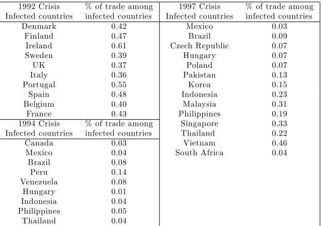
spread of these crises. This is not counterintuitive after inspecting the percentage of trade

among the infected countries for each crisis episode, see appendix. The …gures show that,

for the 1994 and 1997 crises, trading activity (based on imports and exports) among infected

countries is smaller than that between infected countries and their non-infected trading

partners. For the 1992 crisis, trading activity among infected countries is much higher.

Similar …gures are observed in the case of exports only (results not shown). According to

these results trade, whether based on imports and exports or on exports only, appears to be

a statistically signi…cant channel in the transmission of the 1994 currency crisis. There is no

such evidence in the case of the 1992 and 1997 crises.

Table 5: Posterior summary estimates for the coe¢cient of the varous trade covariates

1992 1994 1997

Imports and Exports Mean 6.19 -30.95 -4.07 Median 6.32 -25.15 -3.02 90% CI (-1.66,13.94) (-74.52,-2.08) (-17.16,5.13)

Exports

Mean 8.51 -48.87 -9.17 Median 8.36 -36.53 -4.76 90% CI (-0.85,18.09) (-125.43,-1.95) (-38.48,5.10)

Financial Covariates Financial covariates for the 1994 and 1997 crises are constructed

based on two sets of bi-annual banking data from the Bank of International Settlements (BIS)

beginning in 1988, namely international lending from the international consolidated statistics

and international borrowing from the locational international banking statistics. As in the

case of trade, we constructed three year averages based on those years typically immediately

preceding the crisis date. This resulted in 124 and 136 countries for the 1994 and 1997 crisis,

respectively. We employ three commonly used measures for …nancial linkages between the

common lender and crisis countries (see Van Rijckeghem and Weder 2001, Caramazza et al.,

2004, Dasgupta et al., 2011 and Haile and Pozo, 2008, among others). USA and Japan are

the common lenders for the 1994 and 1997 crises, respectively.

(i) A measure of the importance of the common lender to the crisis country, that is the

proportion of borrowing from a common lender, given by F1i = bi;c=bi, where bi;c is total

(ii) A measure of the importance of an a¤ected country to a common lender, that is the

proportion of borrowings of an a¤ected country in the lending portfolio of a common lender,

expressed asF2i =li;c=lc;whereli;c is lending of a common lender to countryi andlc is total

lending of a common lender.

(iii) A measure of competition for funds, that is the extent to which country i competes

for borrowings from the same common lender as the ground zero country, given by

F Ci = X

c

x0;c+xi;c

x0+xi

1 jxi;c x0;cj

xi;c+x0;c

; (9)

where 0 denotes the ground zero country, cis the common lender, xi;c is total lending from

a countrycto county i, andxi is total borrowings of country i:The higher the value ofF Ci,

the greater the competition for funds between countries i and 0.

The transmission rate from an ‘infectious’ country i to a ‘susceptible’ country j, _ij,

is given by ij = NG + L1(i;j in the same region) e Zi; where Zi denotes the acting

…nancial covariate either F1; F2, orF C, and the associated coe¢cient.

Table 6 reports the mean, median and 90% credible interval for the posterior distribution

of the coe¢cient associated with the di¤erent …nancial covariates, for the 1994 and 1997

crises. These coe¢cients appear to be largely negative as would be expected. For a given

infected country, the greater the proportion of borrowing from a common lender (F1) or in the lending portfolio of a common lender (F2) the more ‘protected’ that country becomes and so the smaller the probability of transmitting the crisis to other countries. The results

point to a signi…cant role for the common lender e¤ect in the 1994 crisis, when measured by

the F1 covariate.

Table 6: Posterior summary estimates for the coe¢cient of the various …nancial covariates

1994 1997

Mean Median 90% CI Mean Median 90% CI F1 -14.14 -13.10 (-30.75,-0.99) -0.72 -0.16 (-8.89,4.94) F2 -15.40 -13.60 (-39.93,4.63) -9.73 -5.91 (-34.33,5.50) FC -7.98 -7.53 (-19.94,2.66) -2.10 -0.35 (-15.71,4.77)

Trade and Financial Covariates Next we consider including both trade and …nancial

covariates together in the model so that we have _ij = G

e 1Xij+ 2Zi; where X

ij and Zi denote the acting trade and …nancial covariates de…ned as

above, with 1 and 2 being the corresponding e¤ects.

When both trade and …nancial covariates are included in the model simultaneously, the

posterior distributions are wider, as con…rmed by the posterior estimates and associated

credible intervals presented in Table 7. This table shows the estimates for the posterior

distributions of each pair of coe¢cients, 1 and 2; associated with the corresponding trade

and …nancial covariate. Trade refers to the trade shares computed based on the average

of imports and exports. The results based on exports only were qualitatively similar. The

results indicate that, as in the case where a …nancial covariate only is included in the model,

the common lender e¤ect continues to be signi…cant in the 1994 crisis, not only when

mea-sured as the proportion of borrowing of an a¤ected country from the common lender, F1, but also as the proportion of borrowings of an a¤ected country in the lending portfolio of

the common lender, F2. This result appears to overshadow the signi…cant e¤ect found for the trade channel in the 1994 crisis, when only a trade covariate is included in the model.

No signi…cant e¤ect is observed for the 1997 crisis, in line with the earlier …ndings.

Table 7: Posterior summary estimates for the coe¢cients associated with the trade and …nancial covariates

1994 1997

Mean Median 90% CI Mean Median 90% CI Trade -26.83 -18.30 (-85.96,2.35) 5.13 5.96 (-7.87,14.95)

F1 -15.87 -13.81 (-36.75,-2.70) 0.16 0.81 (-6.64,5.09) Trade -34.05 -25.62 (-98.49,0.94) 1.73 3.59 (-16.87,13.16)

F2 -53.03 -39.47 (-152.13,-1.00) -14.56 -4.84 (-60.24,7.22) Trade -23.18 -17.97 (-59.28,0.37) 3.51 4.86 (-10.50,13.76)

F C -10.45 -8.95 (-27.90,0.85) -2.25 -1.16 (-12.80,4.26) Note: Trade refers to the shares of the average of imports and exports.

5

Policy Relevance

Understanding how …nancial crises spread, through models such as the one proposed here,

can enhance in the design and evaluation of immunisation policies to reduce the risks and

manage the impact of contagion. So far, at the domestic level, the need for policies aimed at

reducing …nancial fragility has been emphasised; at the international level, the role of better

Chang and Majnoni (2001). The latter can provide liquidity to crisis countries to withstand

pressures of contagion, as witnessed in the recent economic crises, in the form of rescue

packages.

Among the questions increasingly raised on the policy front are how severe is a particular

crisis and how to distribute the available resources to sustain countries that have experienced

or may be experiencing negative outcomes (how many and which countries to support). The

proposed approach can o¤er answers to such questions, as we illustrate below, by drawing

on the past experience of the …ve currency crises episodes analysed earlier. Lessons from

these episodes can o¤er valuable insight to policy makers for future di¢culties.

A number of immunisation policies have been developed, mostly with reference to

epi-demics among humans or animals (Anderson and May, 1991), though examples exist in other

…elds like computer science (Balthrop et al., 2004). The threshold theorem described in

Sec-tion 2.2 provides a natural formulaSec-tion for evaluating this kind of strategies. In particular,

having obtained the parameter estimates of our model, that is the local and global

transmis-sion rates, we can compute the severity measure R , given by (1), for the individual crisis

episodes. Recall that if R > 1 a large number of countries will su¤er from the crisis in question with positive probability, while if R 1only a small number of susceptible coun-tries will ever be a¤ected. Control measures, therefore, typically aim to reduce R below

unity with high probability, which we set to 0.95 in the results that follow. The situation

where a major ‘outbreak’ is unlikely to occur is often referred to as ‘herd immunity’. Having

computedR we can then sample from its posterior density, and estimate the percentage (or

number) of countries to support, denoted by pv, in order to prevent a major crisis. In other

words, we will estimate the smallest pv such that P(R <1) = 0:95.

We will examine here a simple support strategy where the countries to be supported

are chosen uniformly at random. Recall that the threshold parameter without support is

given by R = GE(I)P

jj j j. When a proportion pv of the countries receives support

the threshold reduces to R (pv) = GE(I)

P jj j

P

z j r z_j (1 pv)jpz jv , since the number

of countries prone to the crisis reduces. The percentage pv is computed as the solution to

the equation R (pv) = 1: Thus, pv (and R ) are non-linear functionals of the basic model

parameters, at least when the population structure is non-random and known. Inference

Becker (2000) assuming for simplicity that the outcome within each region is independent

of the fate of other regions. Ball et al. (2004) also consider estimating R and pv using

asymptotic arguments and assumingR >1. The methods considered in this paper are free from these assumptions. Moreover, assuming R > 1 is not particularly satisfactory in our examples, as will soon become apparent. Alternative support policies, like supporting whole

regions chosen at random, are also possible, in which case pv = 1 1=R , see Ball and Lyne

(2006) for a review. In the results that follow we assume that …nancial support to a country

confers complete protection from the crisis, or at least it e¤ectively prevents a particular

country from becoming a¤ected.

Table 8 gives estimates of the posterior mean of R , P(R < 1) and pv. A graph of the

posterior distribution of R for all crisis episodes can be found in the appendix. The mean

posterior estimate for R is greater than one for all episodes. In particular, the posterior

mean of the 1971 and 1973 crises is 2.19 and 2.95 respectively, while that of the nineties

crises is around 1.2. These results corroborate our earlier empirical …ndings relating to

the increasing importance of G; which is now re‡ected in the decreasing length of the 95%

credible intervals forR . The corresponding probability of a crisis being subcritical (‘minor’),

given under the headingP(R < 1), is smaller for the earlier crises compared to the later. In accordance, the associated percentage, pv, of countries to support in order to avoid a major

crisis with a 0.95 probability decreases over time as noted by the …gures in the last column.

The results suggest that the crises of the seventies were of greater severity compared to those

of the nineties.

Table 8: Estimated control measures for the various crisis episodes

Crisis Episode R P(R <1) pv

1971 2.186(0.674,4.610) 0.094 0.291(0.034,0.523) 1973 2.946(0.602,3.632) 0.115 0.265(0.029,0.513) 1992 1.242(0.525,2.425) 0.325 0.240(0.016,0.508) 1994 1.194(0.568,2.170) 0.356 0.230(0.015,0.504) 1997 1.200(0.665,1.938) 0.293 0.210(0.011,0.443)

Note: R measures the severity of the crisis, P(R <1) is the probability that only subcritical (‘minor’) crises can occur and pvis the critical protection coverage i.e. the percentage of countries to support in order to avoid a major crisis with a 0.95 probability. Figures in parentheses are the 95% credibles intervals.

multitype context, though the calculations are somewhat more involving. In the two type

case,R is de…ned as the largest eigenvalue of a matrixM =fmijg; i; j = 1;2;where, crudely

speaking,m12describes the mean number of contacts from countries of type 1 (developed) to

countries of type 2 (developing). More details regarding the computation of themij elements

are given in the appendix.

In addition to the support policy considered above, alternative policies can be

imple-mented that provide partial coverage to more countries as opposed to o¤ering complete

protection to a smaller number. This approach is more involved and additional optimisation

techniques are required. It should be noted that if the local transmission rate is small, as

may be the case in a globalised economy, there will not be a signi…cant di¤erence between

the various adopted policies, at least for homogeneous individuals. Britton and Becker

(2000) consider immunisation strategies within a simpler model, however allowing the level

of susceptibility to the crisis to vary among individuals. Such extensions can be naturally

accommodated within the framework of multitype epidemics discussed earlier.

As demonstrated from the above analysis, the proposed methodology o¤ers a set of

valuable control measures that can be used to analyse contagious …nancial crises. When

implemented in real-time, preliminary estimates of the control measures can be computed

to evaluate prospective immunisation policies and reduce the countries’ vulnerability to

in-ternational contagion, see Fraser et al. (2009) for a recent example on the 2009 in‡uenza

pandemic.

6

Discussion

Crises have been a recurrent feature of …nancial markets for a long time, though it was

primarily the crises of the nineties that sparked increased interest in the study of their

dynamics and propagation. The experience of the recent crises has rekindled such interest,

emphasising the complexity of the …nancial system, and the need for a better understanding

and monitoring of systemic risk and contagious e¤ects.

This paper proposed a modelling framework to analyse …nancial contagion based on

a stochastic epidemic process. The proposed approach directly accounts for the inherent