Munich Personal RePEc Archive
On the estimation of the risk of financial
intermediaries
Delis, Manthos D and Iftekhar, Hasan and Tsionas,
Efthymios
1 September 2012
Online at
https://mpra.ub.uni-muenchen.de/40997/
On the estimation of the risk of financial intermediaries
Manthos D. Delis
Finance Group, Surrey Business School, University of Surrey Guildford, GU2 7XH, UK
E-mail: [email protected]
Iftekhar Hasan
Fordham University and Bank of Finland
1790 Broadway, 11
thFloor,
New York, NY 10019
E-mail:
[email protected]
Efthymios G. Tsionas
Department of Economics, Athens University of Economics and Business 76 Patission Street, 10434 Athens, Greece
E-mail: [email protected]
Acknowledgements: We are grateful to Vasso Ioanidou, James Kolari, Steven Ongena, Laura
On the estimation of the risk of financial intermediaries
Abstract
In this paper we reconsider the formal estimation of the risk of financial intermediaries. Risk is modeled as the variability of the profit function of a representative intermediary, here a bank, as formally considered in finance theory. In turn, banking theory suggests that risk is determined simultaneously with profits and other bank- and industry-level characteristics that cannot be considered predetermined when profit-maximizing decisions of financial institutions are to be made. Thus, risk is endogenous. We estimate the new model on a panel of US banks, spanning the period 1985q1-2010q2. The findings suggest that risk was fairly stable up to 2001 and accelerated quickly thereafter and up to 2007. We also establish that the risk of the failed banks is quite higher than the industry’s average and this risk peaks one to two-years before the default date. Indices of bank risk commonly used in the literature do not capture these trends and/ or the scale of the increase in bank risk. Thus, we provide a new leading indicator, which is able to forecast future solvency problems in the banking industry.
Keywords: Estimation of risk, financial institutions, banks, endogenous risk, US banking sector
1. Introduction
The financial crisis that erupted in 2007 turned the spotlight on financial institutions and their management of the risks they face. A fundamental and timely question is how the risk of a financial intermediary should be measured and the crisis showed that existing measures of the risk of financial institutions are inaccurate and with limited forecasting ability. In this paper, we propose a new method to estimate intermediation risk, using the profit function and the implications of standard economic and banking theory. An important element in our framework is that risk is allowed to be endogenous to internal factors, such as managerial decisions, and external factors, such as the macroeconomic environment. This novelty is essential because existing measures, such as accounting ratios and market rates, cannot capture this type of simultaneity.
Building on economic theory, we use the implications of the portfolio selection models, primarily developed to estimate optimal portfolios by Markowitz (1952) and Roy (1952), and extended by many
others. In this class of models the estimates of the simple variance of profits, or the downside variance, can be used to measure risk. In particular, this theory suggests that if an overall measure of risk is sought in the context of expected utility, that measure should be related to the variability of profits or the variability of factors determining the profit function. In this literature, such measures are employed primarily to model asset prices and portfolio value. Here, we use the profit function to describe the technology of financial institutions in the context of duality theory.
We augment our framework with the implications of intermediation (banking) theory, which suggests that risk decisions of financial intermediaries are simultaneously made with perceptions on expected profits and, in addition, are affected by certain characteristics of a bank’s balance sheet and the state of the economic environment.1 To motivate this, consider two banks with the same initial risk levels but different levels of capitalization or liquidity. Now if e.g. an exogenous or systemic shock hits the banking sector, the more liquid or capitalized bank will be able to buffer risk more easily, while the less
1 This is recognized by Shrieves and Dahl (1992), Diamond and Rajan (2000), Dangl and Zechner (2004), Berger
liquid or less-capitalized bank will have to re-determine its risky position to a greater extent. Naturally, in the following period the level of risk (i.e., the volatility of profits) of the two banks will be quite different. This simultaneity calls for a new model, where risk is jointly determined along with (i) other decisions of the financial institutions (e.g., concerning their level of capitalization and/ or liquidity) and (ii) the macroeconomic environment. In other words, the variability of profits should be endogenous to profits themselves and potentially to other bank-level variables or the structural and macroeconomic conditions. Thus, an important advantage of the approach presented here is that technology, risk, bank decisions and structural and macroeconomic conditions can be modeled simultaneously.
The new method is quite general and can, in fact, be applied to any firm. Here, we focus on financial institutions and, in particular banks, because of the clear implications of banking theory concerning the endogeneity discussed above, the important developments in the banking sector before and after the subprime crisis and the key role banks play in the managerial, the real and the monetary
economic spectrum. One important concern for our modeling choice is not to impose more stringent data requirements on the researcher than the usual bank-level data required for the estimation of the profit function of banks.
increase. Finally, as a robustness check, we demonstrate that our measure predicts the higher risk of banks that became insolvent during our sample period relative to the industry’s average. Given the above, our measure of bank risk is qualified as a new measure for the probability of default and a leading indicator to forecast solvency problems in the banking sector.
As accounting- and market-based measures failed to forecast the financial crisis of 2007, a few recent studies have placed significant effort in revisiting the estimation of bank risk and naturally they relate to our work in a direct way. Most notably, studies like Ioannidou et al. (2009) and Knaup and Wagner (2009) use market- or accounting-based data to evaluate risk. We view these efforts as complementary to ours for two reasons. First, these efforts pose more stringent micro-level data requirements on the researcher or require banks to be listed in the stock market. Second, as an extension to our study, these measures can be compared to ours to show whether findings converge, so that a better measure of total bank risk can be put forth. In a nutshell, we view these developments in the measurement
of bank risk as a significant way to shed some light in this rather neglected modeling issue.
Our study is also related to a big literature on financial stability. For example, Aspachs et al. (2007), within a general equilibrium framework, propose a measure of financial fragility that is based on economic welfare. Also, the set of financial soundness indicators introduced by the IMF in 2006 reflect another step towards a globally accepted measure of financial stability. A number of other indicators are built in empirical studies of financial crises like in Kaminsky and Reinhardt (1999), Elsinger et al. (2006) and Giesecke and Kim (2011). A common feature of these studies is that the indicators sought reflect an aggregate measure of financial stability that incorporates indirect elements of bank risk.
2. Theoretical considerations and empirical facts
2.1. Existing measures of bank risk
It is well-known that the risk of financial institutions (here we refer to banks for simplicity) comes in many types. For example, it takes the form of credit, liquidity, interest-rate, solvency and operational risk. Banks assume all types of risk to make profits. Yet, a bank that undertakes too much risk of any type can become insolvent and fail. For example, high credit and liquidity risks typically manifest themselves through mismatched maturities and durations between assets and liabilities. Also, high operational risk appears when costs are significantly related to bank output. Banks ultimately fail because they cannot generate liquid assets to meet deposit withdrawals, and they operate with insufficient capital to absorb losses if they were forced to liquidate assets. Therefore, a measure of overall bank risk should encompass the features of the various bank risks in one box. For various reasons this box remains somewhat black in the bank-risk literature. In this section, we discuss the theoretical underpinnings of several measures of
risk currently used by researchers and regulators.
For a bank to report higher returns than its peers it must manage the various risks in a better way, or realize market power and other cost advantages compared to its competitors. Aggregate bank profitability is usually measured in terms of the return on assets (ROA = profits/ total assets) or the return on equity (ROE = profits/ total equity). The difference between the two is the so-called equity multiplier (EM = total assets/ total equity), which is the inverse of the basic equity capital ratio. EM (or its inverse) represents a risk measure because it shows how many assets can go into default before a bank becomes insolvent. However, this simple risk measure is problematic in various ways, among which three are the most important. First and foremost, simple accounting ratios do not incorporate expectations concerning the perceived probability of insolvency. In banking markets, probably more intensely than in other sectors, forward-looking expectations are highly important in shaping investors’ behavior, depositors’ confidence and market ratings. A simple accounting ratio fails to account for these expectations as it represents a “static photograph” of a bank’s financial account at a specific point in time. Second, it is
well-known from the portfolio theory that risk is essentially about variability, and more specifically about profit variability. Simple accounting ratios that do not capture variability will fail to highlight the dynamic nature of risk and, therefore, they probably underestimate the risk of insolvency. Finally, under the impulse of the Basel guidelines, capital is heavily regulated, which is a fact that may significantly reduce the importance of the EM ratio as a bank risk proxy.
Other accounting-based ratios used to measure bank risk are related to credit and/or liquidity risk, and mainly include the ratio of (i) non-performing loans to total loans, (ii) loan-loss provisions to total loans, (iii) risk-weighted assets to total assets (regulatory measure) or similar. These measures could ex-post be informative about how risk evolves over time. Yet, besides bearing the significant disadvantages of using accounting data on stock variables to proxy a dynamic element such as risk, these measures do not seem to provide a good ex ante measure of bank risk. Rather, they proxy different aspects of bank risk at a specific point in time and this information comes ex post.
studies represent the first effort to measure the perceived probability of insolvency for each bank in their sample, thus incorporating expectations and variability into their measures. Since insolvency is presumed to occur when current bank losses exhaust capital, estimates of the likelihood of insolvency may be obtained by noting that this likelihood is equivalent to the probability that ROA < -EA, where ROA is as above and EA = 1/ EM. Then, [E(ROA) + EA]/ σ(ROA) represents the number of standard deviations between the expected value of bank profitability, ROA, and that negative values of ROA = -EA that would yield insolvency. Boyd and Rankle (1993) named this estimate of bank risk score” or “Z-index”. The Z-score has been widely used ever since in many empirical studies as a proxy for total bank risk and one may suggest that it has recently become the industry standard, especially when widely available sources of bank data are employed (see e.g. Laeven and Levine, 2009; Demirguc-Kunt et al., 2008; Boyd et al., 2006).
The problem with the Z-score is the calculation of the component of the variance of the returns on
A measure of risk that is quite different in nature involves bank ratings from rating agencies (see e.g. Demirguc-Kunt et al., 2008) and, more appealingly, the disagreement between the major rating agencies (see Morgan, 2002). Rating agencies provide a probability of default, or a similar measure of the ability of a bank to meet its obligations to depositors and other creditors. Thus, ratings may be superior to indicators that use only balance-sheet variables to proxy risk. However, agency ratings have been recently heavily criticized on their ability to estimate and forecast bank risk, especially in the dawn of the global financial crisis (see Felton and Reinhart, 2008). Moreover, relatively small banks that do not trade in the stock market and banks from low-income countries are generally not rated. This poses a heavy data constraint on studies of emerging markets.
Given the problems associated with the above methods, a few very recent studies have come up with new ideas to measure bank risk. Ioannidou et al. (2009) and Jimenez et al. (2009) use ideas stemming from probability of default, VaR and duration methods and analyze the time to default of an
individual loan as a measure of its risk. On the one hand, this duration model has the advantage of providing more accurate information at the very micro level about how risky an individual bank loan is. On the other hand, the method requires market data on individual loans that are not widely available. Another interesting study is that of Knaup and Wagner (2009). Using information impounded in bank share prices and by exploiting differences in their sensitivity to credit default swap (CDS) spreads of borrowers of varying quality, this paper provides a clever new method to proxy credit risk. Note that even though this method has several attractive elements, again the focus is on credit risk and an inherent assumption is that the market for CDS is fully efficient. Also, this method allows evaluation of market risk only for listed banks.
endogenous bank risk, we turn to some stylized facts that show how most of the various existing measures of bank risk discussed here evolve over the period 1985-2010 in the US banking sector.
2.2. Data, stylized facts and measurement of risk with existing techniques
In this section we use bank-level data to construct averages for some of the measures of bank risk that are widely used in the existing empirical literature and show their evolution over time. The first issue is to build a representative dataset. Since the recent crisis originated in the USA, focusing on the US banking sector is a natural choice for a contemporary case study of bank risk. A second issue is the availability of data. The idea here is to develop a new metric for bank risk without posing more stringent data requirements compared to the usual empirical research paper. A quick look in the literature will reveal that the great majority of the empirical papers in this field use either quarterly or annual data. The most widely used database for studies of the US banking system is the one from the FDIC Call reports.
We build an unbalanced dataset that includes information for commercial banks over the period 1985q1-2010q2. We start from the complete sample of banks in the Call reports, but we apply two selection criteria. First, we delete all observations for which data on any of the variables used in our study are missing. Second, we apply an outlier rule to the variables used, corresponding to the 1st and 99th percentiles of the distributions of the respective variables. This deletes extreme values that may drive the results. The final sample consists of 814,253 bank-quarter observations.
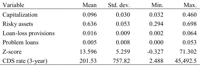
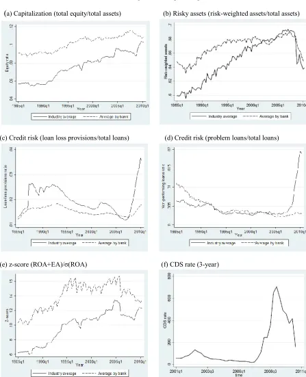
available.2 We report descriptive statistics for the variables in Table 1. Averaging these indices over all banks in the sample on a quarterly basis yields the scores plotted in Figure 1. We name these “averages by bank” and illustrate them by a dashed line. On each graph, we also include the time path of what we refer to as “industry averages”. For this, we calculate the ratio of total industry equity at quarter t to total industry assets at quarter t. We carry out the same calculations for all five ratios. All averages display some in-year volatility due to seasonality of the data that is owing to banks’ accounting practices.3 Evidently, the time paths of averages by bank compared to that of industry averages display some differences, which in some cases are quite significant. Note that empirical studies of the banking industry that employ panel data use bank-level ratios, which are equivalent to our definition of averages by bank, while most of the industry reports use industry averages. Finally, we plot the quarterly average of the CDS rate on Figure 1f.
[INSERT TABLE 1]
[INSERT FIGURE 1]
The bank average of the capital ratio (Figure 1a) shows that equity capital was rising until 2007q3 and only slightly declines up until 2009q4. The increasing trend up to 2007 is due to the higher accumulated wealth of banks in that period and the compliance with Basel capital requirements. Note, however, that the financial crisis erupted in 2007 and, evidently, the capital ratio shows no forecasting ability. This is quite expected because capital erodes only after problems strike, as banks use capital to cover part of their losses. In addition, the decrease in the value of the ratio between 2007q3 and 2009q4 is only 0.008, which is very small in absolute terms compared to the impact the crisis had on the banking sector. The time path of the industry average is similar, except from the period before and after the crisis of 2007-2008. The industry capital ratio peaks at 2005; it starts declining until 2009; and reaches new
2 3-year CDS rates are available for a number of large US banks. We choose the 3-year rates because it has the
largest number of available observations. The quarterly averages of these rates are matched to the full sample of US banks using the so-called cusip number of banks.
3 Given the fact that the relevant literature has not agreed on a unified measure to remove seasonality from
high levels in 2010. This pattern suggests that regulatory compliance and possible capital arbitrage by banks drives the level of capital. In any case, the capital ratio is not informative about bank risk.
Figure 1b shows the equivalent trend in the risk-weighted assets ratio, which is the ratio used by regulators under the impact of Basel guidelines. This ratio is more informative about the adverse developments in 2007 and 2008, while the average by bank and industry average reflect a very similar pattern. The trend of the value of the risky-assets ratio is increasing from 1986q4 to 2007q3 (with a short break between 2001 and 2003) and drops sharply between 2008 and 2010. This shows that banks up to 2007q3 were increasingly using part of their liquid assets to take on more risky projects. However, the risky-assets ratio also has a number of interrelated shortcomings as a measure of risk. The most important of these shortcomings are that (i) risky assets are regulated and this provides banks with incentives to underwrite these assets so as not to exceed the given threshold, and (ii) this ratio does not capture the perceived buildup of risk that led to the financial crisis in 2007.
The loan-loss provisions ratio (Figure 1c) decreases from an average value above 0.018 in 1993q1 to an average value of 0.013 in 1997q3. The ratio returns to a value of approximately 0.018 as of 2010q2. Both this ratio and the risky-assets one show that banks on average were feeling quite safe until well into 2007, taking on extra credit risk and lowering the level of their provisions. Still, the trends in both these measures incorporate or lack all the elements discussed in section 2.1. For example, the increasing trend in the value of the risky-assets ratio might reflect the enhancement of risk-management techniques, while lower values of the provisions ratio might reflect the favorable macroeconomic conditions. Moreover, the fluctuation of the industry average loan-loss provisions is quite immense compared to the bank-level average, which would render results of regressions with the bank-based measure suspect.
reflect the depth of the crisis in the banking sector. In contrast, the industry average reflects a completely different picture, with a sharp rise in non-performing loans starting from 2007q1. We feel that this shows that using a bank-level variable on non-performing loans in bank panel data regression analyses is highly problematic, as this variable greatly underestimates fluctuations in credit risk.
Figure 1e shows the evolution of the average Z-score. Here σ(ROA) at quarter t is calculated using information on ROA from the past 12 quarters. The Z-score is fairly stable in the period 2004-2006 and then falls in 2007 and 2008. The fall in 2007 is relatively large and this shows that the Z-score actually captures the problems of the banking sector in 2007, making this index probably the best among the ones examined previously (at least as far as the stylized facts comply with the crisis). However, the problems discussed above, especially the ones about limited forecasting ability of increasing risk in the period prior to 2007 and the endogeneity of bank risk, remain.
The final graph (Figure 1f) shows the evolution of the average 3-year CDS rate for large rated US
banks over the period 2001q1-2010q2. The picture is very similar to the equivalent for the loan loss provisions and problem loans variables. The CDS rates are very low until 2007, showing no ability to capture the building up of bank risk after 2001. From 2007 onward the rates increase sharply to reach their peak in the first quarter of 2009. Subsequently they decline sharply. As with the two credit risk variables, the problem with this indicator is that it shows no forecasting ability. Further, this and in fact other market measures of bank risk, are only available for a limited number of large institutions. This can be a problem in studies examining issues on regional banking, small enterprise lending, etc.
risk. The next section proposes a new method to estimate the risk of financial intermediaries that accounts for these shortcomings.
3. A new measure of bank risk
A quite important problem faced by the empirical researcher in estimating technology functions of financial intermediaries is that risk should be endogenously determined. The banking theory behind this issue is straightforward. The level of risk is set by bank managers in a way that encompasses information about the level of expected profits, the level of capital and liquidity that banks hold and the state of the structural and macroeconomic environment. Therefore, one cannot suggest that risk determines stricto sensu current bank profits. In fact, the perceived optimal level of bank risk is simultaneously determined
with current profits, also taking into account other endogenous and predetermined variables. This modeling choice is absent in the empirical literature, even though it seems fundamental for the robust
estimation of the risk of financial intermediaries.
Here, we present a model that uses the profit function to estimate endogenous bank profits. We
model a representative bank, but this model may in fact be applied in its general form to any firm.4 Bank risk depends on certain endogenous variables and it is itself considered to be endogenous in the profit function. The rest of the endogenous variables are determined in the context of a simultaneous equation model, and also depend on profits as well as risk. Therefore, the model is very general, as it considers all potential types of endogeneity.
We consider a restricted normalized profit function of the form:
1 1 2
i i i i i
y
x
z
v
, for i1,...,N , (1)where
y
i represents profit of bank i,x
i1 is a standardk
1
1
vector of covariates in the profit function,z
iis a
G
1
vector of endogenous variables,v N
iiid~
0,1
is the error term, and
i2 is the variance of4 Of course, this holds given the alterations that should be made to reflect the special features of the industry
profits to be estimated. Following the portfolio selection theory, we consider the estimates of profit variability σ as a formal measure of risk.5
Assume the following additional specification for the variance of the profit function:
2
( , ),
i
f z
i
(2)where
z
i is aG
1
vector of variables that determines the risk of banks,
is a vector of parameters tobe estimated and
f z
( , )
i
is a functional form differentiable inz
i. For example, f can take the form2
i zi
or 2exp( )
i
z
i
, etc. Note that, despite the fact that we use a “cross-sectional notation”,panel data models of the form 2
2 2
, 1 ,, ,..., ;
it f zit i t i t L
are fully nested within our generalspecification in Eq. (2). This also includes the formal possibility of incorporating fixed effects in (1) and
(2). The dependence on bank profits
y
i will be discussed below.Up to this stage, we formally identify risk with the variability of profits and explain this
variability in terms of a vector of variables included in
z
i. If these variables were predetermined orexogenous, estimation of the profit function in (1) subject to (2) would be straightforward using the method of maximum likelihood. Unfortunately, this is a very strong assumption for financial institutions’
risk-setting behavior, since the
z
is represent firm (bank) characteristics that are simultaneouslydetermined with the level of risk in the following way:
2 2
( , , )
i i i i
z f x y
, (3)where
x
i2 is ak
2
1
vector of explanatory variables of z, which can includex
i1. For example, bank managers set the optimal level of risk given the levels of capitalization, liquidity, etc, which are naturallyincluded in z. This simultaneity of the
z
is with bank risk is a notorious element in the banking literatureand should be accounted for in any attempt to estimate risk robustly. Further, risk and other characteristics of bank balance sheets are heavily affected by the regulatory or macroeconomic conditions prevailing at
each point in time. Therefore, these elements might also have to be included in z. Thorough discussions of these issues can be found in the literature cited in footnote 1.
To account for this endogeneity, assume the following general simultaneous equation model:
22 1 1 2 2
i i i i i
z x
y
u ,
u N
iiid~
0,
, (4)Here,
1 and
2 are known univariate differentiable functions (for example
j
w
w
or
log
j
w
w
, j1, 2),
1,
2 areG
1
vectors of coefficients, and
and
areG G
and2
G k
, respectively. Of course, restrictions are assumed in place for
and
in view of identification.For example, the diagonal elements of
are assumed to be equal to 1 and this matrix must benonsingular. Moreover, the variance 2
i
may depend also onx
i2. Further, the variance may also depend on yi. The Jacobian of transformation from vi to yi can be formally computed andthis possibility has beenrecognized before by Rigobon (2003). This is very important, because the researcher does not need to
identify a set of instrumental variables that are not correlated with vi; the xi1 and xi2 themselves are valid instruments.
For simplicity, we can write
2 * *2 1 1 2 2 2
i i i i i i i
z x
y
u x u . To begin with,
we assume
1
2
0
G1. Then
2
1/ 2
1 1 2
22
|
2
exp
2
i i i i i i
i
y
x
z
p y z
(5)and
/ 2 1/ 2 1
* *
1 * *
2 2
2
2 G exp
i i i i i
p z
z x z x
(6)
1 2
2
( 1)/2 1/2 1 1/2
* * 1 * *
1
2 2
2
; .
.
,
2
exp
2
;
exp
i
G i i i
i i
i
i i i i
x z
y f z
z x x
y
p
z
f
z
z
(7)This likelihood function can be maximized using standard numerical techniques. Formal concentration
with respect to parameters
* and
is also possible, so the problem can be simplified in terms of maximizing the log-likelihood function of the sample.6In the general case, where
1,
2
0
, the formulation ofp y z
i|
i
is straightforward, but theformulation of the inverse distribution
p z y
i|
i
orp z
i is not trivial. The Jacobian of transformationis given by
/ 2 2 2
1 1 2, ;
; ,
G
i i i
i i
i i i
v u f z
D f z
y z z
, (8)
after accounting for the fact that the variance depends itself on endogenous variables (the
z
is). If2
i zi
, then
i;
i
f z
z
. If
2
exp
i
z
i
, then
i;
exp
i i
f z
z
z
.In this case, we have
2
( 1)/ 2 / 2 1 1
1/ 2 1 * * 1 * *
2 2 1 1 2 2 2 2
2
, 2 ; exp
2 ;
; exp .
G G i i i
i i i
i i
i i i i
i
y x z
p y z f z
f z f z
z x z x
z
(9)The simplest case is when
1
w
2
w
w
,7 and
;
i i
f z
z
. In this case the Jacobianterm is simply
2
1 2
, where
2
and
1 2
are rank-oneG G
matrices. Of course, if
1 or6 The details are available on request from the authors. 7 One may think that specifying φ
2(w) = log(w) is better, since variances are restricted to being positive. This is, of
2
(or possibly both) are zero, further simplifications arise. The typical case is to have profits,y
i, andthe variance, 2
i
, appearing as determinants of thez
is. Part of the reason may be that not all banks havepositive profits, so that we cannot consider the log of
y
i. However, one may have
2
w
log
w
, with
12
w
w
. In that case, the Jacobian would be
1
2 1 2
;
;
i i i i f zz
D
f z
. (10)In terms of our model, it is instructive to provide a simple example to show that risk can also be a
function of profits (
y
i). Indeed, consider for simplicity the following “mean-scale” model
i i i
y
y v
, wherev N
iiid~
0,1
. Apparently, the Jacobian of transformation is
2y
y y
v
y
y
(11)and the density of y would be
2 1/ 2 2 22
exp
2
y
y
y y
p y
y
y
. (12)The Jacobian is nonzero, provided
y
is not a solution of the difference equation
y
y y
0
, that is
y 2 should not be equal to C y
2, where C is a constant.Other specifications for the variance term would be acceptable, for example
y 2 C C y1 2
2,1
0
C
. This shows that, in terms of our model, risk can be a function of profits (y
i) themselves, despiteprofits.8 Suppose, indeed, that 2
i zi yi
. Then, relative to (8), the only difference is that theJacobian term is
2 2
1 1 2 2
2 . If
2
0
, the new formulation does not add anythingto the Jacobian, otherwise, the contribution depends on
i, ;
i
if z y
y
.The above describes the equivalent to GARCH-type process for the variance, which is probably enough for practical purposes. In case one wants to extent this case to the stochastic risk or stochastic volatility of the profit function, we provide the analytics in the Appendix. Here we move on to the estimation of the model provided above using data from the US banking sector.
4. Empirical application to the US banking sector
4.1. Empirical setup
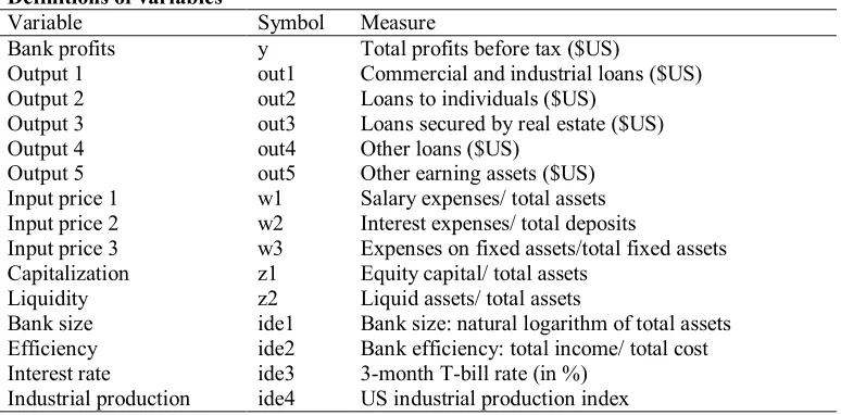
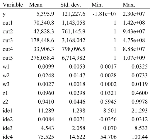
Following the paradigm of Humphrey and Pulley (1997), Koetter et al. (2011) and many others, we use an alternative profit function that models profits as a function of outputs and input prices. The alternative profit function is suitable to measure the extent to which a bank generates maximum profits given its output levels. We provide formal definitions for the variables used to estimate the profit function in Table 2 and summary statistics in Table 3. To define outputs and input prices we follow the intermediation approach (Sealey and Lindley, 1977; Koetter et al., 2011). Under this approach, a bank's production function uses labor and physical capital to attract deposits. The deposits are used to fund loans and other earning assets. Therefore, various categories of loans and other earning assets serve as bank outputs, while relevant ratios of salary expenses, interest expenses and expenses on fixed assets serve as input prices. In essence, our approach considers the measurement of on-balance sheet risk. One could also include a disaggregation of securities and non-interest income or off-balance sheet items as outputs. This would reduce the time frame of the analysis from 1997 onwards, because data on these items are not
8 This is different from a GARCH-M type model, where the lagged variance, typically, enters into the mean
available before 1997. Changes in average values of estimated risk are not larger than 5%, thus, we choose to use the full sample period as benchmark.
[INSERT TABLES 2 & 3] Given the above, we rewrite Eqs. (1) to (3), as:
5 2 2
0
1 1 1
i k i l i m i i i
y
out
z
w
v (13)2
( , )
i
f z
i
(14)2 2
( , , )
i i i i
z f x y
. (15)Eq. (13) is the general form of the alternative profit function to be estimated and Eqs. (14) and (15) are the equivalent ones of Eqs. (2) and (3), respectively. In this system of equations, y is profits before tax,
out represents the five bank outputs listed in Table 2, z, σ and xi2 are as above, and w represents the three input prices defined in Table 2. All variables are in logs.
We estimate the system of Eqs. (13) to (15), using the full-information maximum likelihood method proposed above. We experiment with both a log-linear and a translog specification for the profit function. Further, we impose linear homogeneity by dividing profits and input prices by w3. As profits contain both positive and negative values, taking logs of profits becomes an issue. We, primarily, use the
approach of Bos and Koetter (2011). Under this approach, we impose y = 1 for all y < 0 and construct a negative profit indicator variable, say y1 = |y|, which we use as an additional right-hand side variable.
Following relevant literature, we check the sensitivity of our results by (i) using only positive profits and (ii) adding up the maximum negative profits observed in our sample to all banks plus 1 (to make an index of only positive profits) and (iii) using a non-log specification. We report the results from the method of Bos and Koetter (2011) and the rest are available on request.
liquidity ratio (liquid assets to total assets, denoted as z2). Therefore, we assume that banks make risky decisions simultaneously with the levels of capitalization and/ or liquidity in their balance sheets. Consider, for example, two banks with the same initial risk levels, but different levels of capitalization or liquidity. Now if there is a systemic event in the banking sector, the more liquid or capitalized bank will be able to buffer the risk associated with this event more easily, while the less liquid or less-capitalized bank will have to re-determine its risky position to a greater extent. Naturally, in the following period the level of risk (i.e., the volatility of profits) of the two banks will be quite different. The same will happen if the change in risk comes from a change in operational risk (e.g., an internal organizational event). Many other similar arguments can be found in Freixas and Rochet (2008) and Degryse et al. (2009).9
We identify z in Eq. (15) using a number of variables x2. As discussed in Section 3, these variables can also determine the variance of profits or profits themselves in Eqs. (13) and (14), respectively. This implies that they do not have to be uncorrelated with the error term of Eq. (13). We
name these variables “identifiers”. We run many alternative specifications, but we resort to the inclusion of the fourth lags of bank size and efficiency that are observed at the bank-level, as well as the first lags of the three month T-bill rate and the industrial production index as macroeconomic determinants of bank risk. Concerning the bank-level identifiers the inclusion of bank size and efficiency is a reasonable assumption in the literature of the determinants of bank capital and liquidity (e.g., Flannery and Rangan, 2008; Berger and Bouwman, 2009). In particular, larger and more efficient banks are usually more closely followed by market investors. Thus, these banks may have better access to wholesale liabilities, loan sale markets, liquid assets and so forth. With better access to these liquidity sources, larger banks may therefore require to hold less capital and liquidity. Alternatively, larger banks have more complex balance sheets and are more closely regulated. Thus, these banks might be optimally financed with a larger proportion of equity capital or might need a higher portion of liquid assets to meet unexpected demand. The two bank-level identifiers, denoted as ide1 and ide2, are lagged four times, as we assume that bank
9 One can in fact assume that the volatility of bank profits is endogenous to a number of other bank characteristics.
managers shape their capital and liquidity levels based on information on their size and efficiency in the previous year.10
The two macroeconomic variables, denoted ide3 and ide4, enter Eq. (3) lagged once (values of the previous quarter) to allow information to reach the market. By including these variables we capture the fact that bank managers shape their risky behavior by observing, inter alia, the state of the macroeconomic environment. One can very easily experiment with many other variables common to all banks to be included in Eq. (15) and examine the sensitivity of the results. We experiment with some regulatory dummies, characterizing major regulatory events, with institutional variables, etc. The results are unaffected and, as our main effort here is to estimate risk and not analyze an exhaustive list of its determinants, we decided to keep the empirical framework as simple as possible.
4.2. Empirical results
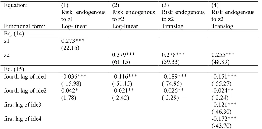
Table 4 reports estimation results for the main variables of interest that help identifying Eqs. (14) and (15), namely z1, z2 and ide1 to ide4. Reporting all estimated coefficients is impractical, as the number of estimated parameters for both the basic log-linear and the translog models is quite high. The results on the rest of the parameters are available on request. We report the results for four specifications. The first two are log-linear specifications and the last two are translog specifications. All variables are statistically significant and bear the expected sign. In particular, banks with higher levels of capital and liquid assets (higher z1 and z2, respectively) take on higher risk in the next period. This is intuitive because most banks tend to mitigate the effects of the increase in capital levels by increasing asset-risk posture, while banks holding a high level of liquid assets tend to use excess liquidity to take on higher risks in the next period.11
[INSERT TABLE 4]
10 We use the values in the previous year and not the ones in the previous quarter to treat problems arising from the
seasonality of bank-level data (see also Delis et al., 2011).
11 For a thorough analysis on the potential positive relationship between risk and capital, see Shrieves and Dahl
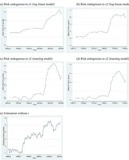
The results of main interest are those on the variance of the profit function, which in our model represents individual bank risk. In Figures 2a to 2d, we plot the quarterly average of the bank-quarter values of risk (log of variance) obtained from the four specifications separately and in Figure 3 we place them together for comparative purposes. Irrespective of the functional form used, or whether we specify z1 or z2 as endogenous, bank risk was fairly stable until 2001 and increased more than 200% thereafter. This pattern is robust to the inclusion of equity capital or a time trend also in Eq. (1), and alternative determinants of z1 or z2 in Eq. (3). Therefore, all models capture the perceived increase in bank risk that took place in the period following the attack on the World Trade Center and prior to 2007.
[INSERT FIGURE 2] [INSERT FIGURE 3]
Specifically, a number of recent studies suggest that certain exogenous shocks, that lead to lower informational asymmetries, trigger intensified competition and credit expansion, and create incentives for
banks to search for higher yield in more risky projects. Rajan (2006) goes on to state explicitly that the source of such bank behavior could be an environment of low interest rates and Delis et al. (2011) confirm this theoretical argument using a similar dataset to the one of the present study. Other scholars (e.g., Stiglitz, 2009) argue that increasing bank risk prior to 2007 is largely attributed to increased political pressure to finance the economy in general and the housing market in particular, and to consumers’ choices to lower the widening income inequality of the time. Our new measure of bank risk largely confirms these perceptions.
US banking sector as early as 1989. The capital requirement does not allow bank capital to fluctuate as much as liquidity, which is subject to only limited regulation. Therefore, bank liquidity is, probably, the most important factor in determining bank risk and is the one used in the rest of the specifications reported in Table 4.12
The second difference comes from using a translog specification, as opposed to a log-linear one. The flexibility of the translog profit function captures a decline in the variability of profits after the eruption of the crisis in 2007 (see lines 3 and 4). This looks sensible, as banks started lowering their exposure to very risky assets, as soon as they could after the eruption of the crisis, while prudential regulation became tighter with an increased number of inspection audits and sanctions. However, we should note that risk remains quite high, compared to the period before 2001. Given the above evidence, we favor the translog specification.
We also estimate a simple model, where the variance is not endogenous to any variables. This is
equivalent to the estimation of Eq. (13) alone and the derivation of the variance of profits therefrom. We average the estimates of the variance across quarters and we plot them in Figure 2e. This specification does capture an increase in bank risk after 2001 and a decrease in 2007. Yet, the time pattern of this line is quite different, showing a large increase in 1992. Not incidentally, Basel I was enacted in 1992, which shows the very special role of considering endogenous variables like capital and liquidity when estimating bank risk. Also, similar to the accounting-based measures, the index reflects some seasonality, which is not smoothed out by endogenous decisions of bank managers. Thus, the model where risk is not endogenous to bank characteristics is systematically different and largely fails to capture all elements explaining the level of bank risk.
Overall, the value of the new method proves quite significant if one compares the results from the proposed method with the indices of bank risk shown in Figure 1. As we discuss in Section 2, these measures fail to consider the endogeneity of bank risk to other bank characteristics and do not capture the
12 An alternative would be to use the distance of equity capital from the minimum requirement. When doing so, the
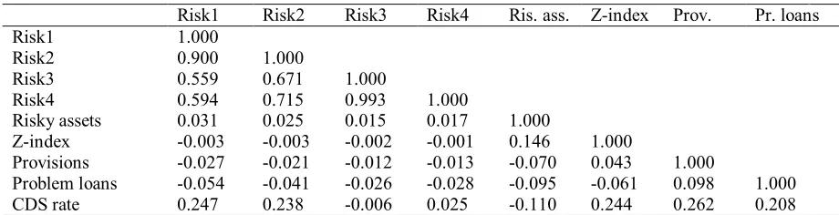
increase in bank risk or the extent of this increase after 2001 and before 2007. Further, in Table 5 we report simple correlation coefficients between the values of the four newly constructed indices (Risk1 to Risk4) and the five existing indices (Risk-weighted assets, loan-loss provisions, problem loans, Z-index and CDS rates). Evidently, correlation coefficients between the newly constructed indices and the existing ones are very low. This is especially true for our preferred measures of risk that come from the translog specification. We attribute the limitations of existing indices (i) to the fact that they do not follow standard economic theory (with the exception of the Z-index), (ii) to the fact that they reflect a static picture of accounting data and (iii) to their inability to account for the endogeneity/ simultaneity issue discussed in this paper.
[INSERT TABLE 5]
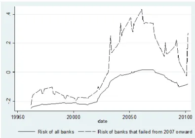
A final, yet important, exercise comes from examining the behavior of banks that at some point during our full sample period became insolvent. Intuitively, the risk of these banks prior to their default
first two quarters of 2010). Notably, FDIC data suggests that 294 more banks failed between 2010q1 and 2012q3.
[INSERT FIGURE 4]
5. Conclusions
This study proposes a new method for the estimation of the risk of financial institutions, which is very general and can be applied to any firm. Two important and interrelated features of the model are that it is based on standard economic and banking theory and that risk is endogenously determined with certain characteristics of the intermediary and with the macroeconomic environment. The model proposes the derivation of bank risk using the variance of the profit function. The profit function is estimated simultaneously with a function of determinants of the variance of profits. In turn, these determinants are also endogenous to the variance of profits and potentially to other bank and industry characteristics,
making all the variables characterizing banking fundamentals, which appear in the estimated system of equations, endogenous. Therefore, the model overcomes the notorious difficulties stemming from the fact that risky decisions of banks are made endogenous to other bank and industry fundamentals.
previous literature on bank risk, and its determinants, questionable. Further, by matching the risk measures obtained from our method with information for the banks that failed, we show that our measure is a good proxy for default risk. The fact that default risk for the banks that subsequently failed peaks one to two years before the period 2008-2010, when most of the bank failures occurred, also shows that power of the new method to forecast problems in the banking sector.
Besides the banking firm, this model can be applied to any other type of financial intermediary or any other non-financial firm, of course with minor modifications pertaining to the special features of each industry. Further, the model can be very easily used to calculate downside variance or look at the standard deviation of expected profits in a fashion similar to the Sharpe ratio. We leave these ideas for future research.
Appendix A. The case of stochastic risk
A process for the variance as proposed in Section 3 is, perhaps, enough for practical purposes. However, one may want to explore the implications of stochastic risk or stochastic volatility for the profit function.
Suppose we have a stochastic risk process of the form
log
i2
z
i
i, where the new error term is
2
~
0,
iid
i
N
. Here, we explicitly assumelog ( , )
f z
i
z
i
. The full model can now be written asfollows:
1 1 2
i i i i i
y
x
z
v
,
22 1 1 2 2
i i i i i
z x
y
u , (A1)
2
log
i
zi
i.In that form, we can formally consider volatility, log 2
i
, as an endogenous (but latent) variable.
2
2
, ,
, ,log , ,
, ,log
i i i i i i i i i
i i i
v u p y z p v u
y z
. (A2)
After computing the Jacobian term, the joint distribution is the following:
1/ 2
2
* * 1 * *
1 1
2 2
2 2
1/ 2 / 2 2 / 2
2 2 2 2
1 1 2 2 2 1 1
1 2 2 2 2 exp exp 2
, ,log
2
2
log
exp
2
i i i
i i i i
i
G G
i i i i i i
i i
y
z z
p y z
e
x
z
x
x
z
(A3)where 1
1 1 2
i i i i i
e
y
x
z
. The simplest case is to have2
1
, so that the Jacobian isindependent of 2
i
. But still the density of the observables is
,
, ,log 2
2i i i i i i
p y z
p y z
d
, (A4)which cannot be computed analytically. For details, see the literature on stochastic volatility. Of course, if
2
1
, the integral is even more complicated and standard simulation techniques proposed in theReferences
Aspachs, O., Goodhart, C.A.E., Tsomocos, D.P., Zicchino, L., 2007. Towards a measure of financial fragility. Annals of Finance 3, 37-74.
Berger, A.N., Bouwman, C.H.S., 2009. Bank liquidity creation. Review of Financial Studies 22, 3779-3837.
Berger, A.N., Humphrey, D.B., 1997. Efficiency of financial institutions: International survey and directions for future research. European Journal of Operational Research 98, 175-212.
Bos, J.W.B, Koetter, M., 2011. Handling losses in translog profit models. Applied Economics 43, 307-312.
Boyd, J.H., De Nicolo, G., Jalal, A.M., 2006. Bank risk-taking and competition revisited: New theory and new evidence. IMF Working Paper WP/06/297.
Boyd, J.H., Runkle, D.E., 1993. Size and performance of banking firms. Testing the predictions of theory.
Journal of Monetary Economics 31, 47-67. Cochrane, 2007. Portfolio theory. Mimeo.
Dangl, T., Zechner, J., 2004. Credit risk and dynamic capital structure choice. Journal of Financial Intermediation 13, 183-204.
Degryse, H., Kim, M., Ongena, S., 2009. Microeconometrics of Banking: Methods, Applications and Results. Oxford University Press, Oxford.
Delis, M.D., Kouretas, G., Tsoumas, C., 2011. Anxious periods and bank lending. MPRA Paper 32422, University Library of Munich, Germany.
Delis, M.D., Hasan, I., Mylonidis, N., 2011. The risk-taking channel of monetary policy in the USA: Evidence from micro-level data. MPRA Paper 34084, University Library of Munich, Germany. Demirguc-Kunt, A., Detragiache, E., Tressel, T., 2008. Banking on the principles: Compliance with Basel
Elsinger, H., Lehar, A., Summer, M., 2006. Risk assessment for banking systems. Management Science
52, 1301-1314.
Flannery, M.J., Rangan, K.P., 2008. What caused the bank capital build-up of the 1990s? Review of Finance 12, 391-429.
Freixas, X., Rochet, J.C., 2008. Microeconomics of Banking. MIT Press, Cambridge, Massachusetts. Giesecke, K., Kim, B., 2011. Systemic risk: What defaults are telling us. Management Science 57,
1387-1405.
Hannan, T.H., Hanweck, G.A., 1988. Bank insolvency risk and the market for large certificates of deposit. Journal of Money, Credit, and Banking 20, 203-211.
Humphrey, D.B., Pulley, L.B., 1997. Banks' response to deregulation: Profits, technology and efficiency.
Journal of Money, Credit and Banking 29, 73-93.
Ioannidou, V., Ongena, S., Peydro, J.L., 2009. Monetary policy, risk-taking and pricing: Evidence from a
quasi-natural experiment. Discussion Paper 2009-31S, Tilburg University, Center for Economic Research.
Jiménez, G., Ongena, S., Peydró, J.L., Saurina, J., 2009. Hazardous times for monetary policy: What do twenty-three million bank loans say about the effects of monetary policy on credit risk-taking? Banco de España Working Papers 0833, Banco de España.
Kaminsky, G.L., Reinhart, C.M., 1999. The twin crises: The causes of banking and balance-of-payments problems. American Economic Review 89, 473-500.
Knaup, M., Wagner, W., 2009. A market-based measure of credit quality and banks' performance during the subprime crisis. European Banking Center Discussion Paper No. 2009-06S. Available at SSRN: http://ssrn.com/abstract=1274815.
Koetter, M., Kolari, J.W., Spierdijk, L., 2011. Enjoying the quiet life under deregulation? Evidence from adjusted Lerner indices for U.S. banks. Review of Economics and Statistics, forthcoming.
Markowitz, H., 1952. Portfolio selection. Journal of Finance 7, 77-91.
Mitchell, D.W., 1982. The effects of interest-bearing required reserves on bank portfolio riskiness.
Journal of Financial and Quantitative Analysis 17, 209-216.
Mitchell, D.W., 1982. Some regulatory determinants of bank risk behavior. Journal of Money, Credit, and Banking 18, 374-382.
Morgan, D.P., 2002. Rating banks: Risk and uncertainty in an opaque industry. American Economic Review 92, 874-888.
Reinhart, C., Felton, A., 2008. The first global financial crisis of the 21st Century. MPRA Paper 11862, University Library of Munich, Germany.
Rigobon, R., 2003. Identification through heteroskedasticity. Review of Economics and Statistics 85, 777-792.
Roy, A.D., 1952. Safety first and the holding of assets. Econometrica 20, 431-449.
Sealey, Jr.C.W., Lindley, J.T., 1977. Inputs, outputs, and theory of production cost at depository financial institutions. Journal of Finance 32, 1251-1266.
Shrieves, R.E., Dahl, D., 1992. The relationship between risk and capital in commercial banks. Journal of Banking and Finance 16, 439-457.
Table 1
Summary statistics of variables commonly used as measures of bank risk
Variable Mean Std. dev. Min. Max.
Capitalization 0.096 0.030 0.032 0.460 Risky assets 0.636 0.053 0.294 0.698 Loan-loss provisions 0.016 0.009 0.002 0.064 Problem loans 0.005 0.008 0.000 0.053
Z-score 13.596 5.259 -0.327 71.302
Table 2
Definitions of variables
Variable Symbol Measure
Bank profits y Total profits before tax ($US)
Output 1 out1 Commercial and industrial loans ($US) Output 2 out2 Loans to individuals ($US)
Output 3 out3 Loans secured by real estate ($US) Output 4 out4 Other loans ($US)
Output 5 out5 Other earning assets ($US) Input price 1 w1 Salary expenses/ total assets Input price 2 w2 Interest expenses/ total deposits
Input price 3 w3 Expenses on fixed assets/total fixed assets Capitalization z1 Equity capital/ total assets
Liquidity z2 Liquid assets/ total assets
Bank size ide1 Bank size: natural logarithm of total assets Efficiency ide2 Bank efficiency: total income/ total cost Interest rate ide3 3-month T-bill rate (in %)
Table 3
Summary statistics
Table 4
Estimation results on the main determinants of risk
Equation: (1)
Risk endogenous to z1
(2)
Risk endogenous to z2
(3)
Risk endogenous to z2
(4)
Risk endogenous to z2
Functional form: Log-linear Log-linear Translog Translog Eq. (14)
z1 0.273***
(22.16)
z2 0.379*** 0.278*** 0.255***
(61.15) (59.33) (48.89) Eq. (15)
fourth lag of ide1 -0.036*** -0.116*** -0.189*** -0.151*** (-15.98) (-51.15) (-74.95) (-55.27) fourth lag of ide2 0.042* -0.021** -0.026** -0.024**
(1.78) (-2.42) (-2.29) (-2.24)
first lag of ide3 -0.121***
(-46.30)
first lag of ide4 -0.172***
(-43.70)
Table 5
Correlation matrix between indices of bank risk
Risk1 Risk2 Risk3 Risk4 Ris. ass. Z-index Prov. Pr. loans
Risk1 1.000
Risk2 0.900 1.000
Risk3 0.559 0.671 1.000
Risk4 0.594 0.715 0.993 1.000
Risky assets 0.031 0.025 0.015 0.017 1.000
Z-index -0.003 -0.003 -0.002 -0.001 0.146 1.000
Provisions -0.027 -0.021 -0.012 -0.013 -0.070 0.043 1.000
Figure 1
Evolution of various bank risk indices over the period 1985q1-2010q2
(
a) Capitalization (total equity/total assets) (b) Risky assets (risk-weighted assets/total assets)
(c) Credit risk (loan loss provisions/total loans) (d) Credit risk (problem loans/total loans)
(e) z-score (ROA+EA)/σ(ROA) (f) CDS rate (3-year)
Figure 2
Evolution of bank risk (log of variance) over the period 1985q1-2010q2
(a) Risk endogenous to z1 (log-linear model) (b) Risk endogenous to z2 (log-linear model)
(c) Risk endogenous to z2 (translog model) (d) Risk endogenous to z2 (translog model)
(e) Estimation without z
Figure 3
Evolution of bank risk (log of variance) over the period 1985q1-2010q2
Figure 4