The Evolution of Taxes and Hours Worked in Austria, 1970 2005

Munich Personal RePEc Archive

The Evolution of Taxes and Hours

Worked in Austria, 1970-2005

Dalton, John

Wake Forest University

May 2012

Online at

https://mpra.ub.uni-muenchen.de/48222/

The Evolution of Taxes and Hours Worked in Austria,

1970-2005

∗

John T. Dalton

Wake Forest University

First Version: July 2008

This Version: May 2012

Abstract

Aggregate hours worked per working-age person decreased in Austria by 25% from 1970 to 2005. During the same time period, taxes increased, particularly the effective marginal tax rate on labor income. Using a standard general equilibrium growth model with taxes, I quantitatively assess the role played by the evolution of taxes on the evolution of hours worked in Austria. The model accounts for 76% of the observed decrease in hours worked per working-age person. My results are in line with other studies, such as Prescott (2002), which find taxes play an important role in explaining aggregate hours worked.

JEL Classification: E24, J22, E13

Keywords: taxes, labor supply, growth accounting, dynamic general equilibrium

∗_{I thank Tim Kehoe for his advice and constant encouragement.}

1

Introduction

In examining the causes of the differences in aggregate hours worked both across countries and

within countries over time, macroeconomists find taxes play an important role. Prescott (2002)

and Prescott (2004) argue tax rates account for much of the difference observed in hours worked

between the United States and Europe. Ohanian, Raffo, and Rogerson (2006) expands Prescott’s

work to a larger set of countries over a longer time span and finds much of the variation in hours

worked over time and across countries can be explained by taxes. Conesa and Kehoe (2008) take

a more detailed look at the cases of Spain and France and also show taxes play an important

role in explaining the fall in hours worked.

I build on the existing literature by analyzing the specific case of aggregate hours worked in

Austria over the years 1970-2005. Austria is representative of the experience of many European

countries. In 1970’s Austria, hours worked per working-age person were higher than in the United

States. By the year 2005, hours worked per working-age person in Austria had decreased by

25% and stood at a level lower than that in the United States. I study the question, “How well

can the evolution of taxes account for the evolution of aggregate hours worked in Austria?”

This paper closely relates to the work in Conesa and Kehoe (2008), essentially applying

the methodology employed in that paper to the case of Austria over the period 1970-2005. The

methodology used is the one developed by Kehoe and Prescott (2002) to study great depressions

and is based on growth accounting and the dynamic general equilibrium growth model. Kehoe

and Prescott (2007) contains a collection of papers employing a similar framework to study

sixteen depressions throughout history and the world, including the cases of France, the United

States, Japan, and Mexico. Cicek and Elgin (2011) represents a more recent application of

this methodology for the case of Turkey. There are three steps to the methodology. First,

growth accounting quantifies the contributions of total factor productivity (TFP), capital, and

aggregate hours worked for the growth of output. Second, the neoclassical growth model serves

as a theoretical framework for understanding the dynamics of the economy. The central feature

of the model is a representative household which takes the evolution of taxes and TFP as given

and chooses sequences of consumption, hours worked, and capital to maximize utility. Third,

experiments generate model data which can then be compared to the actual data observed in

the economy. As Kehoe and Prescott (2002) point out, the methodology functions as a diagnostic

tool, relying on macro data and a macro model to determine the factors of the economy requiring

more detailed study.

The growth accounting for Austria reveals a large divergence between TFP and output per

working-age person. The divergence results from the steady decline in hours worked in Austria

from 1970 to 2005. Austria contrasts with the experience of the United States. In the United

States, hours worked per working-age person remain fairly constant and have even increased since

the early 1980’s. The growth accounting for Austria is, however, in line with other European

countries experiencing large declines in hours worked, such as Spain, France, and Finland.1

I find the neoclassical growth model augmented with taxes does a good job of replicating the

data from my growth accounting exercise. In order to perform this experiment, I exogenously

set the consumption tax rate and the effective marginal tax rates on labor and capital income

to the rates found in the data. The model with these actual tax rates accounts for 76% of

the fall in hours worked observed in Austria over the period 1970-2005. I show the necessity

of augmenting the model with the sequences of actual tax rates by conducting two additional

experiments which fail to replicate the experience of the Austrian economy. The first tests the

performance of a model with no taxes against the data, while the second tests a model with

constant tax rates. Both of these experiments fail to match the data as well as the model with

the sequences of the actual tax rates found in the data. My results support the evidence found

in the literature mentioned earlier.

I do not wish to claim other labor market frictions or institutions play no role in explaining

the evolution of hours worked in Austria. However, as Conesa and Kehoe (2008) point out,

to the extent that the development of such institutions coincides with the increase in taxes,

these explanations would be correlated with the evolution of taxes in Austria. My analysis

also says nothing about the distribution of hours worked within the working-age population.

For example, labor force participation among the elderly remains low in Austria. The pension

system in Austria is one of the more generous and complete in Europe, widely recognized as

1

unsustainable, and currently in a state of on-going reform.2

I return to this point when discussing

avenues for future research in the concluding remarks of this paper.

The remainder of the paper is organized as follows: Section 2 contains the growth accounting

exercise. In Section 3, I describe the neoclassical growth model with taxes. Section 4 presents

the calibration and results of the numerical experiments. Section 5 concludes.

2

Growth Accounting

The growth accounting for Austria is based on the standard theoretical framework of the

neo-classical growth model, as in Kehoe and Prescott (2002), and is intended to detect deviations

from balanced growth behavior. The model contains an aggregate production function taking

the Cobb-Douglas form,

Yt =AtK α tL

1−α

t , (1)

whereYt is output,At is TFP,Kt is capital input,Lt is labor input, and 1−αis labor’s share of

income. If both the growth in TFP and the growth in working-age population, Nt, are assumed

to be constant,

At+1 =g 1−α

At, (2)

Nt+1 =ηNt, (3)

then there is a balanced growth path where output per working-age person, Yt

Nt, grows at the rate g−1; the capital-output ratio, Kt

Yt, is constant; and hours worked per working-age person,

Lt

Nt, are constant.

Kehoe and Prescott (2002) then rewrite the aggregate production function (1) as the

follow-ing:

Yt

Nt

=A

1 1−α

t

Kt

Yt ₁α

−α L_t

Nt

, (4)

2

Figure 1: United States Growth Accounting D 1 1 t

A

1960 1965 1970 1975 1980 1985 1990 1995 2000 2005

t t

N

Y

which decomposes output per working-age person, Yt

Nt, into a productivity factor,A

1 1−α

t ; a capital

factor, Kt

Yt

₁α

−α

; and a labor factor, Lt

Nt. On a balanced growth path, growth in output per working-age person arises from changes in the productivity factor, as both the capital and labor

factors remain constant. In order to show the usefulness of this decomposition, consider the

case of the United States. Figure (1) reports the data for the United States over the period

1960-2005. Growth in the United States appears close to balanced, particularly over the period

1960-1983. During these years, growth in Yt

Nt is close to growth in A

1 1−α

t , while Kt Yt ₁α −α and Lt

Nt remain fairly constant. However, after 1983, the United States growth path becomes less balanced. Yt

Nt grows faster thanA

1 1−α

t , which is driven by the gradual increase in Lt

Nt.

In order to perform the growth accounting decomposition for Austria, data needs to be

collected for the series of output, capital stock, working-age population, and hours worked. A

value for labor’s share of income also needs to be assigned. The series of TFP can then be

information on the data used throughout this paper and their sources.

The national accounts for Austria do not report a series for the capital stock, so I construct

the series using the perpetual inventory method,

Kt+1 = (1−δ)Kt+Xt, (5)

whereδ denotes a constant depreciation rate of capital and Xtis investment. The capital stock

series can then be accumulated from data on investment and values forδ and an initial capital

stock. The value of δ is chosen to match the average ratio of depreciation to gross domestic

product (GDP) in the data over the calibration period 1970-2005. In Austria, the average ratio

of depreciation to GDP over the years 1970-2005 is

1 36

2005

X

t=1970

δKt

Yt

= 0.1388. (6)

The value of the initial capital stock is chosen so that the capital-output ratio in the initial

period, 1960, matches the average capital-output ratio over a reference period, 1961-1970:

K1960

Y1960 = 1

10 1970

X

1961

Kt

Yt

. (7)

The equations (5), (6), and (7) make up a system that can be solved to find the capital stock

series and the value of δ. The calibrated value for δ in Austria is 0.0382.

The labor income share can be measured directly from the Austrian data over the years

1970-2005. My calculations for the labor income share yield an average value of 0.6896, which

translates into a capital income share, α, of 0.3104. The Austrian value of the capital income

share is in line with the results in Gollin (2002), which suggest a common value ofα= 0.3 across

countries.

Only the TFP series remains to be calculated in order to report the growth accounting for

Austria. This is done by simply rearranging the aggregate production function (1) and using

the measures of output, capital stocks, hours worked, and the labor income share to solve for

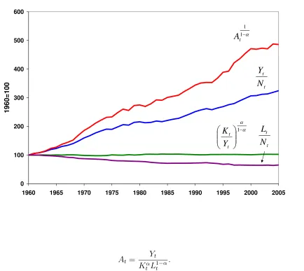
Figure 2: Austria Growth Accounting 0 100 200 300 400 500 600

1960 1965 1970 1975 1980 1985 1990 1995 2000 2005

1 9 6 0 = 1 0 0 D 1 1 t

A

N

Y

N

L

At =

Yt Kα tL 1−α t . (8)

Figure (2) displays the growth accounting decomposition (4) for Austria over the period

1960-2005. Three observations are of note. First, the overall effects of the AustrianWirtschaftswunder

are clearly present. Austrian output per working-age person, Yt

Nt, grows at an average annual rate of 2.7% over the entire period 1960-2005. During the years 1960-1980, a period coinciding

more closely with the actualWirtschaftswunder, growth in Yt

Nt is even faster, averaging an annual rate of 3.9%. Second, in contrast to the United States experience, the Austrian growth path

displays large deviations from balanced growth after 1965, as evidenced by the divergence of

output per working-age person, Yt

Nt, and the productivity factor, A

1 1−α

t . Third, this deviation

from balanced growth occurs due to the steady fall in aggregate hours worked per working-age

person, Lt

working-age person in Austria is in line with the experiences of other European countries. This

paper’s main purpose is to understand the role played by taxes in explaining the decrease in

hours worked in Austria by testing a model with taxes against the data presented in this growth

accounting exercise. I now turn to describing such a model.

3

Model

The economic environment is that of the simple dynamic general equilibrium model augmented

with taxes. A representative household takes the evolution of taxes and TFP as given and

chooses sequences of consumption, hours worked, and capital to maximize utility. A

represen-tative firm produces output with an aggregate technology, taking prices as given. Government

collects proportional taxes on consumption, labor income, and capital income and rebates the

proceeds to the household in a lump-sum fashion, making sure to balance its budget.

Specifically, the representative household chooses sequences of aggregate consumption, Ct;

aggregate capital stocks,Kt; and aggregate hours worked,Lt, to solve the following maximization

problem:

max ∞

X

t=To

βt

γlogCt+ (1−γ)log(¯hNt−Lt)

(9)

s.t. (1 +τtc)Ct+Kt+1 = (1−τ

l

t)wtLt+ [1 + (1−τ k

t)(rt−δ)]Kt+Tt, (10)

Ct, Kt, Lt≥0, (11)

Lt≤¯hNt, (12)

KTo given, (13)

where β, 0< β < 1, is the discount factor; γ, 0< γ <1, is the consumption share; and ¯h is an

individual’s time endowment of hours available for market work. Equation (10) represents the

household’s budget constraint. τc t, τ

l

t, and τ k

t are the tax rates on consumption, labor income,

and capital income. wtandrtare the wage rate and rental rate. δ, 0< δ <1, is the depreciation

rate. Tt is the lump-sum transfer from the government. The inequalities represented in (11) are

constrains the household’s choice of aggregate hours worked, since the total number of hours

available for work is ¯hNt. Finally, (13) is the constraint on the initial stock of capital.

The representative firm produces output according to the production technology (1). A

competitive environment, in which the firm earns zero profits and minimizes costs, gives rise to

the pricing rules for the wage rate and rental rate:

wt= (1−α)AtK α tL

−α

t , (14)

rt =αAtK α−1

t L

1−α

t . (15)

The feasibility constraint in the economy requires current output be divided between

con-sumption and investment:

Ct+Kt+1−(1−δ)Kt=AtK α tL

1−α

t . (16)

The government’s budget constraint ensures the total tax receipts exactly equal the

lump-sum transfers to the household:

τtcCt+τ l

twtLt+τ k

t(rt−δ)Kt=Tt. (17)

Note that the assumption about government transfers matters. Rebating all the tax receipts in

a lump-sum fashion to the household is equivalent to viewing government expenditure as a

sub-stitute for private consumption. For instance, the tax revenue might be used to finance health

care, unemployment insurance, or public schools. Specifying the government in this way leads

changes in taxes to have larger effects on the supply of labor, as discussed in Prescott (2002).

However, this assumption is reasonable as long as tax revenue is mainly used to finance

substi-tutes for private consumption, which is the case in Austria. Figure (3) shows the sum of health,

education, and social protection expenditures as a percent of total government expenditure in

Austria over the years 1995-2005. On average, health, education, and social protection account

for 60% of government expenditure. The data in Figure (3) are likely a lower bound estimate

of government substitutes for private consumption, since they do not include such potentially

Figure 3: Government Health, Education, and Social Protection Expenditure in Austria 55 56 57 58 59 60 61 62 63 64 65

1995 1996 1997 1998 1999 2000 2001 2002 2003 2004 2005

P e rc e n t o f T o ta l G o v e rn m e n t C o n s u m p ti o n services.

Now, an equilibrium for this environment can be defined as follows:

Given sequences of TFP,At; working-age population, Nt; consumption tax rates,τ c t;

labor income tax rates, τl

t; and capital income tax rates, τ k

t, for t = To, To+ 1, ...

and an initial capital stock, KTo, an equilibrium with taxes is sequences of aggregate

consumption, Ct; aggregate capital stocks, Kt; aggregate hours worked, Lt; wages,

wt; interest rates,rt; and transfers,Tt, such that the following conditions hold:

1. Given wages, wt, and interest rates, rt, the representative household chooses

consumption, Ct; capital, Kt; and hours worked, Lt, to maximize utility (9)

subject to the budget constraint (10), the nonnegativity constraints (11), the

upper bound on the total number of hours worked (12), and the constraint on

2. The wages, wt, and interest rates, rt, and the representative firm’s choices

of labor, Lt, and capital, Kt, satisfy the cost minimization and zero profit

conditions (14) and (15).

3. Consumption, Ct; labor, Lt; and capital, Kt, satisfy the feasibility constraint

(16).

4. Government transfers, Tt, satisfy the government’s budget constraint (17).

These equilibrium requirements reduce to a system of equations which characterizes the

equilibrium. Taking the first-order conditions of the household’s maximization problem, I solve

for the household’s intertemporal and intratemporal conditions:

Ct+1

Ct

=β 1 +τ

c t

1 +τc t+1

[1 + (1−τtk+1)(rt+1−δ)], (18)

(1−τtl)wt(¯hNt−Lt) =

1−γ

γ (1 +τ

c

t)Ct. (19)

Plugging the firm’s optimality conditions (14) and (15) into the household’s optimality conditions

(18) and (19), yields

Ct+1

Ct

=β 1 +τ

c t

1 +τc t+1

[1 + (1−τtk+1)(αAt+1K

α−1

t+1 L 1−α

t+1 −δ)], (20)

(1−τtl)(1−α)AtK α t L

−α

t (¯hNt−Lt) =

1−γ

γ (1 +τ

c

t)Ct, (21)

which, combined with the feasibility constraint (16) and government budget constraint (17), is

the system of equations characterizing the equilibrium of the model. I use this system when

computing the equilibrium of the model in my numerical experiments.3

3

4

Numerical Experiments

The numerical experiments I perform compare the data to three theoretical economies with

different tax scenarios. The first is a model with no government and no taxes at all in which

τc t, τ

l

t, and τ k

t equal zero every period. The second is a model with constant taxes in which τ c t,

τl

t, and τ k

t are set to the rates observed in the data in 1970. The third is a model with taxes

in which the evolution of τc t,τ

l

t, andτ k

t follows the actual evolution of the rates as measured in

the data. The theoretical economies will determine the equilibrium evolution of the endogenous

variables given a set of calibrated parameters and the evolution of the exogenous variables. The

exogenous variables are the sequences of TFP, working-age population, and the taxes rates. The

numerical experiments will then allow me to compare the evolution of the aggregate variables

implied by the model with those actually observed in the data. The aggregates I compare are

real GDP per working-age person, the capital-output ratio, and, of course, hours worked per

working-age person.

4.1

Calibration

Following the methodology in Mendoza, Razin, and Tesar (1994), I use data on aggregate tax

collections to calculate the sequences of effective tax ratesτc t,τ

l

t, andτ k

t. However, I follow other

recent macroeconomic studies in deviating from the procedure in Mendoza, Razin, and Tesar

(1994) in two important respects.4

First, I attribute a fraction of household’s non-wage income

to labor income. Second, I measure effective marginal tax rates instead of effective average tax

rates.

The theoretical framework developed in Section 3 motivates the choice of focusing on effective

marginal tax rates. The representative household’s decisions take place at the margin, as shown

in equations (20) and (21). Given the progressivity of income taxes, the estimates of the income

taxes need to be adjusted. In principle, I should use micro data, such as a representative sample

of tax records, to estimate effective income tax functions to perform my adjustments. Conesa

and Kehoe (2008) does exactly this for the case of Spain. Conesa and Kehoe (2008) multiplies

4

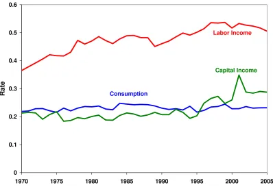
Figure 4: Effective Marginal Tax Rates in Austria

0 0.1 0.2 0.3 0.4 0.5 0.6

1970 1975 1980 1985 1990 1995 2000 2005

R

a

te

Labor Income

Consumption

Capital Income

average income taxes by a factor of 1.83 to obtain marginal tax rates for Spain. In the case

of Austria, I simply follow Prescott (2002) and Prescott (2004) for the United States case and

multiply average income taxes by a factor of 1.6 to obtain marginal tax rates. Conesa, Kehoe,

and Ruhl (2007) adopt the same procedure for the case of Finland. Figure (4) graphsτtc,τ l t, and

τk

t for Austria over the period 1970-2005. A key observation in Figure (4) is that the effective

marginal tax rate on labor income trends upward over the 35 year period, from a low of 0.36 in

1970 to a high of 0.54 in 1997. Detailed information on the construction of the tax rates appears

in the appendix.

The exogenous series of TFP in the experiment with no government and no taxes is calculated

from equation (8) in the growth accounting exercise. In the experiments with taxes, I adjust

the series of TFP by modifying equation (8) to

At =

Ct+Xt

Kα tL

1−α

t

whereCt+Xt is real GDP at factor prices in the data. However, when I report the contribution

of TFP to growth in the results section, I report the conventional measure of TFP,

ˆ

At =

ˆ

Yt

Kα tL

1−α t

, (23)

where

ˆ

Yt= (1 +τ c

¯

T)Ct+Xt (24)

is real GDP at market prices of the base year ¯T = 2000.

The exogenous sequence of the working-age population is that measured from the data in

the growth accounting exercise. I assign a value of ¯h= 100 for an individual’s time endowment

of hours available for market work per week.

The remaining parameters are the initial capital stock, KTo; capital share, α; depreciation

rate, δ; discount factor,β; and consumption share, γ. The initial capital stock is the 1970 value

from the series of capital stocks calculated in the growth accounting exercise. The capital share

and depreciation rate are also the same as in the growth accounting exercise, which means α=

0.3104 and δ = 0.0382. Rearranging equations (18) and (19) allows me to calibrateβ and γ as

follows:

β = (1 +τ

c

t+1)Ct+1 (1 +τc

t)Ct

1 1 + (1−τk

t+1)(rt+1−δ)

, (25)

γ = (1 +τ

c t)Ct

(1 +τc

t)Ct+ (1−τtl)wt(¯hNt−Lt)

. (26)

I calculate a vector of β’s and γ’s for the same period used to calculate δ and α, 1970-2005,

and then take the average of these vectors to assign values to β and γ. The calibrated values

of β and γ vary depending on the tax scenario of the numerical experiment. In the experiment

with no taxes, β = 0.9830 and γ = 0.2418. In the experiment with constant taxes, β = 1.0023

and γ = 0.3682. In the experiment with the actual tax rates,β = 1.0030 and γ = 0.4163. The

calibrated values for β in the experiments with taxes are both greater than 1, which means the

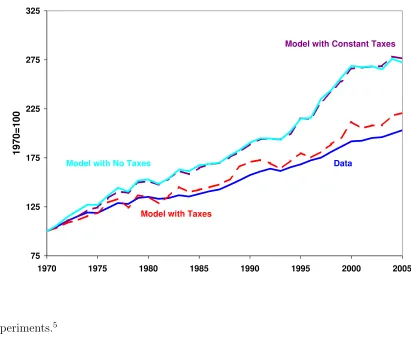
Figure 5: Real GDP per Working-Age Person in Austria

75 125 175 225 275 325

1970 1975 1980 1985 1990 1995 2000 2005

1

9

7

0

=

1

0

0

Data

Model with Taxes

Model with Constant Taxes

Model with No Taxes

tax experiments.5

4.2

Results

Figures (5) - (7) and Table (1) compare data from the Austrian economy with the corresponding

results from the numerical experiments. Figure (5) compares the growth of the Austrian economy

from 1970 to 2005 with the growth of the three theoretical economies over the same period. The

growth in the model with no taxes is similar to that in the model with constant taxes. Both

the model with no taxes and the model with constant taxes predict a noticeably larger increase

in real GDP per working-age person than actually occurred in Austria. The model with taxes,

however, predicts a path for real GDP per working-age person which is much more in line with

the actual experience of the Austrian economy. This result suggests the models based on the

evolution of TFP alone are inadequate for understanding recent growth in Austria. Indeed, the

5

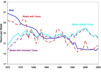
Figure 6: Hours Worked per Working-Age Person in Austria

17 19 21 23 25 27 29

1970 1975 1980 1985 1990 1995 2000 2005

H

o

u

rs

p

e

r

W

e

e

k

Data

Model with Taxes

Model with No Taxes

Model with Constant Taxes

graph highlights the importance of recognizing the role played by the evolution of taxes in the

Austrian economy since 1970.

Figure (6) compares the data on the evolution of hours worked per working-age person in

Austria with the results implied by the three theoretical economies. The model with no taxes

fails to account for the fall in hours worked seen in the data. The series of hours worked

generated by the model with no taxes remains fairly constant. The model with constant taxes

does not improve the performance of the model. The key point here is that the mere presence

of distortions are not enough to generate the evolution of hours worked seen in the data. The

actual evolution of taxes is important for generating the fall in hours worked, as seen by the

series implied by the model with taxes. Figure (6) shows the model with taxes does a good job

accounting for the magnitude of the decrease in hours worked in Austria from 1970 to 2005.

In the data, hours worked per working-age person in Austria fall by 25% from 1970 to 2005,

Figure 7: Capital-Output Ratio in Austria

2.5 2.7 2.9 3.1 3.3 3.5 3.7 3.9 4.1 4.3

1970 1975 1980 1985 1990 1995 2000 2005

R

a

ti

o

Data

Model with Taxes Model with Constant Taxes

Model with No Taxes

seems to qualitatively match the evolution of hours worked in the data, though the hours worked

in the model with taxes fluctuate more than those in the data. The qualitative similarities are

evident if the series in Figure (6) are divided into four period: 1970-1985 coincides with a steady

fall in hours worked, hours worked remain constant or increase during the years 1985-1992, the

years 1992-1997 see another fall in hours worked, and 1997-2005 is another period of roughly

constant hours worked. These four periods are also identifiable in the series of labor income tax

rates presented in Figure (4).

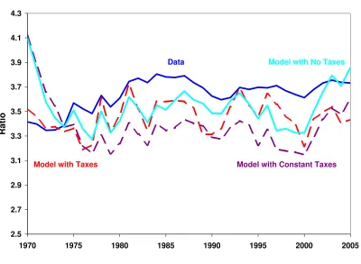
All three models predict similar results with respect to capital deepening. Figure (7) graphs

the evolution of the capital-output ratio in Austria and the capital-output ratios implied by

the three numerical experiments. The three models generate smaller capital-output ratios than

those found in the data.

Finally, Table (1) presents the quantitative implications of the numerical experiments by

Table 1: Decomposition of Average Annual Changes in Real GDP per Working-Age Person in Austria (Percent)

Data No Taxes Constant Taxes Actual Taxes

1970-2005

Change in Y/N 2.03 2.86 2.90 2.26

Due to TFP 2.75 2.75 2.78 2.90

Due to K/Y 0.11 -0.08 -0.17 -0.03

Due to L/N -0.83 0.20 0.30 -0.61

theoretical economies. For ease of exposition, I take the natural logarithm of equation (4):

logYt

Nt

= 1

1−αlogAt+ α

1−αlog Kt

Yt

+ logLt

Nt

. (27)

Output per working-age person now decomposes into three additive factors. The numbers in

Table (1) can be viewed as growth rates, as they are average annual changes multiplied by 100.

5

Conclusion

The workhorse of modern macroeconomics is the general equilibrium growth model. It has been

used to study business cycles, monetary policy, great depressions, and a host of other economic

issues. I apply the model to the study of the Austrian economy. Calibrated to the Austrian

experience, a simple dynamic general equilibrium growth model with taxes can account for 76%

of the decrease in hours worked per working-age person observed in Austria over the years

1970-2005. My results support the conclusions of recent studies stressing the importance of taxes in

explaining the evolution of hours worked.

Two extensions of my work come to mind, one immediate and one an avenue for future

research. First, I have not included a sensitivity analysis for the assumptions unique to my

analysis. In particular, the preference specification gives rise to macro elasticities which some

consider too high. This is a common complaint of macro models of this type. Rogerson and

Figure 8: Life Cycle Employment Profiles Relative to the United States, 2005

0.0 0.2 0.4 0.6 0.8 1.0 1.2

15-19 20-24 25-29 30-34 35-39 40-44 45-49 50-54 55-59 60-64

E

m

p

lo

y

m

e

n

t-P

o

p

u

la

ti

o

n

R

a

ti

o

Age Germany

Italy

Belgium France

with taxes. Rogerson and Wallenius (2009) find taxes still have large effects on aggregate hours

worked. My assumption about tax revenue being lump-sum transferred to the representative

household could also be subjected to sensitivity analysis. Conesa and Kehoe (2008) conducts an

extensive sensitivity analysis on these assumptions and more in an identical model to the one

presented here. I refer the reader to their discussion.

Second, the analysis presented here is silent about the distribution of hours worked within the

working-age population, as mentioned in Section 1. Recent research stresses the importance of

heterogeneity across individuals in accounting for facts regarding cross-country differences in

la-bor outcomes. Prescott, Rogerson, and Wallenius (2009) present data on life cycle

employment-population ratios in four European countries (Belgium, France, Germany, and Italy) relative

to the United States, reproduced here for the year 2005 in Figure (8), which is consistent with

the implications of their model.6

Prescott, Rogerson, and Wallenius (2009) find employment

6

Figure 9: Life Cycle Employment Profile in Austria Relative to the United States, 2005

0.0 0.2 0.4 0.6 0.8 1.0 1.2

15-19 20-24 25-29 30-34 35-39 40-44 45-49 50-54 55-59 60-64

Age

Employment-Population

Ratio

differences between these European countries and the United States are concentrated among

young and old workers. Austria presents an exception to this finding. Figure (9) reproduces the

same life cycle employment profile used in Prescott, Rogerson, and Wallenius (2009) for the case

of Austria in the year 2005. Employment differences in Austria relative to the United States are

concentrated solely among older workers. This feature of the Austrian data suggests an avenue

Appendix

The growth accounting exercises require the use of national accounts data and data on the

la-bor force. The United States national accounts data are taken from the Bureau of Economic

Analysis’s National Income and Product Accounts, available at www.bea.gov, and the

Interna-tional Monetary Fund’s (IMF)International Financial Statistics CD-ROM. The United States

data on the labor force can be found in the Organisation for Economic Co-operation and

De-velopment’s (OECD) Population and Labour Force Statistics online at www.sourceoecd.com.

National accounts data for Austria are from three sources: the IMF’s International

Finan-cial Statistics, the Detailed Tables of Main Aggregates in the OECD’s Annual National

Ac-counts, and Angus Maddison’s Historical Statistics for the World Economy: 1-2003 AD online

at www.ggdc.net/Maddison. Austrian data on the labor force are from the OECD’sPopulation

and Labour Force Statistics and the Conference Board and Groningen Growth and Development

Centre’s Total Economy Database. The Total Economy Database resides at

www.conference-board.org/economics.

The Austrian data on the composition of government expenditure appearing in Figure (3)

are from the OECD’s General Government Accounts. The General Government Accounts are

also available online at www.sourceoecd.org. Total government expenditure is broken down into

different categories based on the United Nation’sClassification of the Functions of Government.

Given the focus of this paper, a more detailed discussion regarding the construction of

the Austrian tax rates seems appropriate. As mentioned in the text, I follow the procedure

of previous studies, such as Conesa, Kehoe, and Ruhl (2007) and Conesa and Kehoe (2008).

Calculating the effective marginal tax rates requires data on both tax revenue and the tax

base. For the data on tax revenue, I use the OECD’s Details of Tax Revenues of Member

Countries. The tax base data are from theDetailed Tables of Main Aggregates in the OECD’s

Annual National Accounts. Both data sources are available online at www.sourceoecd.org. The

following key defines the variables used to calculate the tax rates:

Tax Revenue Statistics

1100 = Taxes on income, profits, and capital gains of individuals,

2000 = Total social security contributions,

2200 = Employer’s contribution to social security,

3000 = Taxes on payroll and workforce,

4100 = Recurrent taxes on immovable property,

4400 = Taxes on financial and capital transactions,

5110 = General taxes on goods and services,

5121 = Excise taxes,

National Accounts

CH H

t = Household final consumption expenditure,

CN P I SH

t = Final consumption expenditure of nonprofit institutions serving households,

CEt = Compensation of employees,

OSM It= Household gross operating surplus and mixed income,

δKH H

t = Household consumption of fixed capital,

Yt= GDP,

Tt= Taxes less subsidies,

δKt= Consumption of fixed capital.

The consumption tax rates are computed as

τtc =

5110 + 5121

CH H t +C

N P I SH

t −5110−5121

. (28)

In order to construct the tax rates on labor and capital income, I first calculate the marginal

tax rate on household income. Second, I calculate the tax rates on labor and capital income by

assigning the ambiguous income categories in the data to either labor or capital income. I set

capital’s share of income to beα, which is the same as that in the aggregate production function

(1). The marginal tax rate on household income is

τth =adj

1100

CEt−2200 + (OSM It−δKtH H)

, (29)

whereadjis the adjustment factor taking the progressivity of the income taxes into account and

converts the average tax rate to a marginal tax rate. In the case of Austria, I set adj = 1.6.

τtl =

τth[CEt−2200 + (1−α)(OSM It−δK H H

t )] + 2000 + 3000

(1−α)(Yt−Tt)

, (30)

τtk =

τh

tα(OSM It−δKtH H) + 1200 + 4100 + 4400

α(Yt−Tt)−δKt

References

Cicek, D., and C. Elgin (2011): “Not-Quite-Great Depressions of Turkey: A Quantitative

Analysis of Economic Growth over 1968-2004,”Economic Modelling, 28(6), 2691–2700.

Conesa, J. C., and T. J. Kehoe (2008): “Productivity, Taxes and Hours Worked in Spain:

1970-2005,” Working Paper.

Conesa, J. C., T. J. Kehoe, and K. J. Ruhl (2007): “Modeling Great Depressions: The

Depression in Finland in the 1990s,” in T. J. Kehoe and E. C. Prescott, editors, Great

De-pressions of the Twentieth Century, Minneapolis, MN: Federal Reserve Bank of Minneapolis,

427-475.

Gollin, D. (2002): “Getting Income Shares Right,” Journal of Political Economy, 110(2),

458–474.

Hofer, H., and R. Koman (2006): “Social Security and Retirement Incentives in Austria,”

Empirica, 33(5), 285–313.

Kehoe, T. J.,and E. C. Prescott(2002): “Great Depressions of the 20th Century,” Review

of Economic Dynamics, 5(1), 1–18.

(eds.) (2007): Great Depressions of the Twentieth Century. Minneapolis, MN: Federal

Reserve Bank of Minneapolis.

Mendoza, E. G., A. Razin, and L. L. Tesar (1994): “Effective Tax Rates in

Macroe-conomics: Cross-Country Estimates of Tax Rates on Factor Incomes and Consumption,”

Journal of Monetary Economics, 34(3), 297–323.

Ohanian, L., A. Raffo, and R. Rogerson (2006): “Long-Term Changes in Labor Supply

and Taxes: Evidence from OECD Countries, 1956-2004,” NBER Working Paper 12786.

Prescott, E. C. (2002): “Richard T. Ely Lecture: Prosperity and Depression,” American

(2004): “Why Do Americans Work So Much More Than Europeans?,” Federal Reserve

Bank of Minneapolis Quarterly Review, 28(1), 2–13.

Prescott, E. C., R. Rogerson, and J. Wallenius (2009): “Lifetime Aggregate Labor

Supply with Endogenous Workweek Length,”Review of Economic Dynamics, 12(1), 23–36.

Rogerson, R., and J. Wallenius (2009): “Micro and Macro Elasticities in a Life Cycle