Munich Personal RePEc Archive
The dynamic process of economic takeoff
and industrial transformation
Chang, Ming-Jen and Wang, Ping and Xie, Danyang
National Dong Hwa University, Washington University in St. Louis
and NBER, Hong Kong University of Science and Technology
23 February 2011
Online at
https://mpra.ub.uni-muenchen.de/31868/
The Dynamic Process of
Economic Takeo¤ and Industrial Transformation
Ming-Jen Chang, National Dong Hwa University Ping Wang, Washington University in St. Louis and NBER Danyang Xie, Hong Kong University of Science and Technology
February 2011
Abstract: This paper studies the patterns and key determinants of staged economic development. We construct a two-sector dynamic general equilibrium model populated with one-period lived non-overlapping generations, featuring endogenous enhancement in modern technology and endogenous accumulation of labor skills and capital funds. We consider preference biases toward the traditional sector of necessities, capital barriers to the modern sector, and imperfect substitution between skilled and unskilled workers. By calibrating the model to …t historic U.S. development, we …nd that modern technologies, saving incentives and capital fundings are most important determinants of the takeo¤ time. By evaluating the process of economic development, we identify that saving incentives is most crucial for the speed of modernization. We also study how labor and capital allocations toward the modern industry respond to various preference, technology and institutional changes. We further establish that labor, capital and output are most responsive to the initial state of modern technologies but least responsive to the initial state of skills, along the dynamic transition
path. (JEL Classi…cation Numbers: O330, O410)
Keywords: Economic takeo¤ and industrial transformation; endogenous skill and technological advancements; saving incentives, preference biases and capital barriers.
Acknowledgments: We are grateful for valuable comments and suggestions from Eric Bond, Tain-Jy Chen, Michael Song, Hsueh-Fang Tsai, and Henry Wan, as well as seminar participants of Fudan University, Fu-Jen Catholic University, Iowa State University, National Central University, National Chengchi University, National Taiwan University, San Francisco Fed, Wuhan University, the Globalization Conference in Hong Kong, the International Conference in Memory of John C.H. Fei, and the Midwest Macroeconomic Conference. Financial support from Academia Sinica, the Granada Program of the Ministry of Education, the National Science Council (NSC 98-2911-H-001-001), the Research Grants Council of the Hong Kong SAR (RGC HKUST-6470/06H), and the Weidenbaum Center on the Economy, Government, and Public Policy to enable this international collaboration is gratefully acknowledged. The usual disclaimer applies.
1
Introduction
The process of economic development has played a central role in the economics platform. Since
the classic works by Lewis (1955), Rostow (1960), Rosenstein-Rodan (1961), Fei and Ranis (1964),
and Tsiang (1964) more than four decades ago, there have been numerous studies devoting to
understanding the patterns and key determinants of staged economic development. A sample of
issues examined include:
(i) How important is the role of technological advancements played in industrialization?
(ii) Whether are saving incentives more important than skill accumulation in early development?
(iii) Why did some countries, such as the Newly Industrialized Countries (NICs), take o¤
success-fully but not others?
Despite the long tradition over the past …ve decades, not until recently have the aforementioned
issues been addressed within a more rigorous general equilibrium framework. A representative set
of such studies include Goodfriend and McDermott (1995), Fei and Ranis (1997), Laitner (2000),
Gollin, Parente and Rogerson (2002), Hansen and Prescott (2002) and Wang and Xie (2004), to
name but a few. In this paper, we extend the static general equilibrium model of Wang and Xie
(2004) to a dynamic general equilibrium setting, thereby enabling us to examine the dynamic process
of economic take-o¤ explicitly. To fully characterize the dynamic process is by no means an easy
task. The main challenge is: how to design a model to permit an analysis of the global dynamics, as
local transitional dynamics techniques would not suit the purpose of characterizing the long process
of transformation from traditional to modern economies.1
Speci…cally, we maintain several key features considered by Wang and Xie (2004), such as
pref-erence biases (away from the necessary agriculture good), heterogeneous capital costs (between the
agricultural and modern sectors), and imperfect factor substitution (between skilled and unskilled
workers). However, we generalize their static framework by allowing capital funds, labor skills, as
well as sector-speci…c technologies to grow over time, depending on optimizing decisions by
house-holds and …rms. While funds can be accumulated due to intergenerational savings, skills can evolve
due to educational e¤ort. Moreover, the modern technology can be enhanced by inputs of skilled
research labor.
The main message delivered by this research is as follows. The modern industry is more likely
to be activated and the economy can take o¤ at a faster speed when:
(i) the initial level of the modern technology or the speed of modern technology growth is high;
(ii) the initial supply of fund or the subjective intergenerational discounting factor is high, or the
modern sector capital barriers is low;
(iii) the initial fraction of skilled workers or the speed of knowledge accumulation is high, or the
disutility scaling factor is low;
(iv) the preference bias away from the traditional good is low.
The quantitative results suggest that the initial levels of the modern technology and fund supply
as well as the subjective intergenerational discounting factor are most in‡uential for determining
the timing of economic takeo¤ – a 10% increase in each of these three parameters can reduce the
benchmark activation time of 45 years by more than one third.
Moreover, we also …nd in our quantitative analysis that the subjective discounting factor that
a¤ects individual’s saving incentives is most in‡uential in generating a rapid transition toward a
modern society. While the preference bias, the skill accumulation and the capital allocation barrier
are crucial for labor shifts from the traditional to the modern sector, the initial fraction of the skilled
labor, the initial level of fund supply and the initial level of the modern technology are essential for
capital reallocation toward the modern industry.
Finally, by examining the dynamic transition in our model economy, we identify that labor,
capital and output all shift rapidly in response to changes in the initial level of modern technology,
their responses to the initial fraction of skilled labor are more moderate. As a consequence, the
per capita real income growth is most responsive to the initial level of modern technology and least
responsive to the initial fraction of skilled labor.
Literature Review
Goodfriend and McDermott (1995) illustrate that scale economies in production and learning are
crucial for staged economic development, whereas Laitner (2000) argues savings are key elements to
enable an economy to be advanced. While Hansen and Prescott (2002) points out that faster modern
technology adoption and to capital accumulation to explain the delay of modernization. Departing
from the conventional overlapping-generations framework commonly used in this literature, Gollin,
Parente and Rogerson (2002) formulate an in…nite-horizon model that permits an analysis of global
dynamics and illustrate that an initially higher agricultural technology can release resources more
e¤ectively from the agriculture to the modern sector to advance an economy.
In their second book, Fei and Ranis (1997) summarize that the main determinants of economic
development include not only the technologies of the agricultural and the modern sectors but also
the speed of capital accumulation and the ability to reallocate labor from the agriculture to the
modern sector. Wang and Xie (2004) adds to this list that the degree of luxuries of modern products
and the availability of the skilled labor are also crucial for economic take-o¤. In Bond, Jones and
Wang (2005), it is emphasized that learning from exporting can lower unit production costs to
enable activation of more advanced industries. More recently, Tung and Wan (2008) consider
informational problems in a game with …rms interacting with each other sequentially where the
barrier to modernization is due to …rms’ lack of incentives to serve as a pioneer in bringing a new
technology to the society, because the sunk cost incurred for doing so may not be recovered as the
future pro…ts will quickly disappear with new …rms entering the industry.
Our paper contributes to this growing literature in several signi…cant aspects. In contrast with
all other papers except Gollin, Parente and Rogerson (2002) and Bond, Jones and Wang (2005), our
paper permits analytic characterization of the global dynamics of the model to enable a thorough
study of both the dynamic process of economic take-o¤. In contrast with Gollin, Parente and
Rogerson (2002) and Bond, Jones and Wang (2005), we allow modern technology, skills and capital
funds to be endogenously evolved over time and examine the roles of other important
development-driving forces beyond the initial level of agricultural technology.
2
The General Setup of the Economy
We construct a closed economy dynamic general equilibrium model to study the process of economic
take-o¤. There are two di¤erent industries in the model, a traditional industry (industry 1) and
a modern industry (industry 2), respectively. In this general model economy, we assume that the
accumulation of funds and skills are both endogenous. Thus, our general setup may be viewed as
an extension of the static model developed by Wang and Xie (2004) by allowing funds and skilled
More speci…cally, we assume that the traditional industry is using a conventional Cobb-Douglas
technology, but the modern industry exhibits increasing returns to scale at the aggregate level. We
therefore model this feature by resorting to the literature of Marshallian externality in economic
growth theory (Romer 1986, Benhabib and Farmer 1994, Wang and Xie 2004). We have:
Y1t = A1tK1t1L11t 1; (1)
Y2t = A2tK2t2L1
2
2t K1
2
2 ; (2)
where 2> 1. K2t denotes the capital input in a typical …rm and K2 is the industry average and
treated by individual …rms as exogenous given. BothK1tandK2tare fully depreciated in one period.
A1tandA2trepresent the productivity of a speci…c technology used by an unskilled and skilled labor
respectively to produce …nal goods, Y1t and Y2t. If A10 and A2t 1 denote the innovations in the
initial level in industry1and the leading-edge productivity in periodt-1in industry2;respectively,
and LAt denotes the labor work in the research and development (R&D) sector at datet, and then
the innovations of the two industries are as follow:2
A1t = A10(1 + 1)t; (3)
A2t = A2t 1
h
1 + 2 1 e LAt
i
; (4)
where 1; 2 2(0;1), >0 and 0:We will restrict our attention to the case where the speed
of modern technology growthb2= 2 1 e LAt exceeds that of the traditional sector
1, with
2(1 )< 1.
The population of the economy at timetis denoted byNt, which grows at a constant rate,n >0:
Nt=N0(1 +n)t, whereN0 >0. There are two types of workers: skilled (whose supply isNst) and
unskilled (whose supply isNut). Under full employment, we have the following population identity:
Nut+Nst = Nt. At time 0, the initial fraction of skilled workers is given by s = Ns0=N0 > 0.
Denoting t as the (endogenous) e¤ort to acquire skills at timet, we can then specify the supply of
skilled workers as follows:
Nst=Nt
2
41 (1 s)e
t
P
=1
3
5; 0< s <1; (5)
where > 0 measures the speed of knowledge accumulation. Without the consideration of the
endogenous e¤ort of knowledge accumulation, the knowledge accumulation process reduces to that
in Aghion (2002). Our setup of endogenous knowledge accumulation is signi…cantly simpler than
the evolution of human capital in the human capital-based endogenous growth model developed by
Lucas (1988) because we avoid modeling skills as a stock variable.
Assume that only the skilled workers can handle work in R&D sector and industry 2, but all
workers can produce the traditional good in industry 1. Thus, the allocation of skilled and unskilled
labor must satisfy:
L1t+L2t+LAt = Nut+Nst =Nt; (6)
L2t+LAt Nst:
The …rst expression equates labor demand with labor supply in the absence of unemployment. While
the second inequality indicates the demand for labor in the traditional sector cannot exceed total
labor supply, the third restricts the aggregate demand for skilled labor by the modern industry and
R&D.
To endogenize the fund accumulation process, one may follow the conventional optimal growth
framework considering individual’s consumption and saving decisions over time. Alternatively, one
may construct a one-period nonoverlapping-generations setup (Saint-Paul and Verdier, 1993) with
income being divided between consumption and bequests periodically (see Aghion and Bolton, 1997).
While the latter simpli…es the analysis greatly, individuals are short-lived and intergenerational skill
accumulation is di¢cult to be constructed in a convincing manner. In our paper, we follow in the
spirit of the latter setup to simplify the consumption tradeo¤ but allow individuals to be long-lived.
This is done by assuming that a representative agent’s lifetime utility function takes the following
form:
Ut= lnC1t+ ln (C2t+ Nt) + ln(St+ Nt) z
1+
t
1 + ; (7)
where the representative agent chooses whether to enjoy consumption of the traditional and the
modern goods (C1t
Nt and
C2t
Nt) now or to save for the future (
St
Nt).
3 While the traditional good is
assumed a necessity, the modern product is a luxury good so that > 0 captures the preference
bias away from the modern good; that is, the higher is, the less the modern good is necessary to
consumers (see Wang and Xie, 2004). Also, 2(0;1)is a subjective intergenerational discounting
factor. Additionally, the utility cost knowledge accumulation e¤ort takes a simple constant elasticity
3Without loss of generality, the original utility function in per capita form is assumed to be:
lnC1t
Nt
+ ln C2t
Nt
+ + ln St
Nt
+ z
1+ t
1 + ;
of intertemporal substitution form with a convex disutility cost of e¤ort, wherez >0 is a disutility
scaling factor and >0 is the elasticity parameter of e¤ort disutility.4
Denoting t as the (endogenous) rate of savings in proportion to Y2t (Y1t is assumed to be
perishable and can not be saved):
St= tY2t: (8)
Intergenerational savings, St, will be added to the funding supply across generations, that is,
Ft=Ft 1+St; (9)
where Ft 1 measures the beginning-of-lifetime funds supply in the economy. The available funds
can be used to purchase capital. Assuming that installing capital in the modern sector is more
costly, we can then specify the funds (capital) allocation constraint as:
K1t+qK2t Ft 1; (10)
where q > 1 captures the barrier to the allocation of capital to the modern sector.5 As it can be
seen, our model, despite its simplicity, can capture the emphasis by Laitner (2000) that savings play
an important role in the dynamic process of modernization.
In the absence of international trade, goods market must clear sector-by-sector, as given by:
C1t = Y1t(A1t; K1t; L1t); (11)
C2t = (1 t)Y2t(A2t; K2t; L2t): (12)
We can thus rewrite the optimization problem facing the integrated consumer-producer as
fol-lows:
Vt= maxflnC1t+ ln (C2t+ Nt) + ln (St+ Nt) z
1+
t
1 + g;
such that
C1t=Y1t(A1t; K1t; L1t);
C2t= (1 t)Y2t(A2t; K2t; L2t);
St= tY2t(A2t; K2t; L2t);
4Let the market wage bew. Individual optimization then implies that the marginal disutility of e¤ort is equal to the shadow wage: z =w. Taking log and di¤erentiating, one obtains: ddlnlnw =
1
.
K1t+qK2t=Ft 1;
L1t+L2t+LAt=Nt;
L2t+LAt =Nst( t);
A2t=A2t(LAt);
based on which we shall proceed with solving the dynamic competitive equilibrium.
3
Optimization and Equilibrium
We now turn to solving the optimization problem. We begin by deriving conditions under which the
returns on capital and labor are equalized across the two sectors, which are referred to as no-arbitrage
conditions. We then characterize intertemporal tradeo¤s, which pin down the consumption-saving
choice and the knowledge accumulation decision. Finally, we examine when the modern sector
will be activated as an intertemporal equilibrium outcome and when the periodic pro…t becomes
positive.
Adynamic competitive equilibrium is a tuplefC1t; C2t; t; t; St; Nst; Nt; Y1t; Y2t; L1t; L2t; LAt;
K1t; K2t; Ft 1; pt; A1t; A2tg1t=1 such that:
(i) each agent chooses consumption of the traditional and the modern goods as well as
intergener-ational savings and knowledge accumulation e¤ort to maximize the lifetime utility (a total of
four optimization conditions);
(ii) both labor and capital are allocated optimally between di¤erent sectors (a total of three
no-arbitrage conditions);
(iii) sectoral outputs are given by (1) and (2);
(iv) production technologies evolve according to (3) and (4);
(v) intergenerational savings is determined by (8);
(vi) skills and funds are accumulated according to (5) and (9), respectively;
(vii) labor, funds, capital and both goods markets are all clear, i.e., (6), (9), (10), (11) and (12)
There are18equations for eachtand17sequences of endogenous variables in our dynamical system.
One can easily show that one of the equations at each point in time is redundant and the Walras
law is met (speci…cally, when both labor and goods markets are clear, the funds market must also
be clear).
3.1 Skilled Labor No-arbitrage Condition
Let us focus on the case where both sectors are active and the labor market is completely segmented
in the sense that no skill labor works in the traditional sector (i.e.,L2t+LAt=Nst) – we will derive
later the conditions for this case to arise. Under this circumstance, the marginal product of skilled
labor (M P L) must exceed that of unskilled labor.
For any given productivity level A2t, the skilled labors at date t must be indi¤erent between
working at industry 2or at R&D sector. Therefore, the following research production no-arbitrage
equation must hold in equilibrium:
M P L2t=M P LAt;
where, from equations (2) and (4),
M P L2t = (1 2)A2tK2tL2t 2;
M P LAt = 2 A2t 1e LAtK2tL12t 2:
The no-arbitrage condition can thus be written as:
(1 2)
h
1 + 2(1 e LAt)i=
2 e LAtL2t;
L2t=
(1 2)
2
h
(1 + 2)e LAt
2
i
; (13)
which together with equation (5) yields the fraction of research labor:
(1 2)
2
h
(1 + 2)e LAt
2
i
+LAt=Nt
2
41 (1 s)e
t
P
=1
3
5; (14)
from which one can solve forLAt =Qt(Nt;f gt=1;s; ; 2; ; ; 2), which depends positively on
the endogenous knowledge accumulation e¤ort. From (13),
L2t=
(1 2)
2
h
(1 + 2)e Qt
2
i
: (15)
Hence,
@L2t
@Qt
= (1 2)(1 + 2)
2
e Qt;
Also, equation (14) implies:
@Qt
@ t =
(1 s)Nte
t
P
=1
(1 2)
2 (1 + 2)e
Qt + 1
t(f gt=1;s; ; 2; ; ; 2): (16)
Intuitively, an increase in the fraction of research labor generates two opposing e¤ect on the
fraction of skilled labor in modern good production: (i) by labor substitution, less skilled labor is
allocated to modern good production and (ii) by skill accumulation, more skilled workers become
available. As a result, the relationship between the fraction of skilled labor in modern good
pro-duction and the fraction of research labor need not be monotone. It is clear that the fraction of
research labor depends positively on endogenous knowledge accumulation e¤ort ( ). Until
knowl-edge accumulation e¤ort is pinned down, one cannot easily characterize the fraction of research
labor.
3.2 Capital No-arbitrage Condition
Substituting the funds allocation constraint (with equality) into the …rst-order conditions with
respect toK1t and K2t implies:
t= 1 +
(1 ) Nt
(1 + )A2tK2tL12t 2
; (17)
K1t=
q 1
2(1 t)+ 2 t
(1 t)A2tK2tL
1 2 2t + Nt
A2tL12t 2
: (18)
The …rst equation illustrates consumption-intergenerational saving tradeo¤, which can be best
elab-orated by Figure 1. Speci…cally, the marginal bene…t of intergenerational saving as a result of
al-truistic preferences must be equal to its marginal cost measured by foregone consumption. We can
then obtain the expression for funds allocated to the modern sector:
K2t= Ft 1
q
2 1 Nt
2(1+ )A2tL
1 2 2t
1 + 1
(1+ ) 2
: (19)
The condition forK2t>0 requires:
Ft 1
q >
2 1 Nt
2(1 + )A2tL12t 2
together with the implicit restriction that t>0, namely,
(1 ) >
Nt
A2tK2tL12t 2
; (21)
which both hold if = 0 (i.e. the sector 2 will be activated immediately if = 0). When is
positive, then activation can take place ifA2t and L2t eventually become large to outweigh Nt.
3.3 Intertemporal Tradeo¤ Conditions
Under our setup, the consumption-saving tradeo¤ is parsimonious as there is no need for deriving
the Benveniste-Scheinkman condition associated with states variables in dynamic programming.
Moreover, the knowledge accumulation decision is also simple because it is in terms of e¤ort without
any feasibility condition accompanied.
pt=
M U2t
M U1t
= A1tK
1
1tL
1 1
1t
(1 t)A2tK2tL12t 2 + Nt
= Y1t
(1 t)Y2t+ Nt
: (22)
3.3.1 E¤ort toward Knowledge Accumulation
The …rst-order condition for knowledge accumulation e¤ort t is:
M B
= t f gt=1;s; ; 2; ; ; 2
1 1
L1t
+
[ L2t+ (1- 2)]
1- 2
L2t
(1- t)Y2t
(1- t)Y2t+ Nt
+ (1- 2)
L2t
tY2t tY2t+ Nt
1- 1
L1t
= z t =M C : (23)
[image:12.612.140.545.414.500.2]This condition equates the marginal bene…t of knowledge accumulation e¤ort with its marginal cost.
Figure 2 illustrates the determination of knowledge accumulation intuitively, where the marginal
bene…t is decreasing in knowledge accumulation e¤ort and the marginal cost is increasing in it. In
response to a reduction in Y1t ors, the marginal bene…t of accumulating knowledge rises, thereby
increasing the speed of knowledge accumulation and the supply of skilled labor. An increase in
Y2t or a decrease in creates a direct positive e¤ect on the marginal bene…t as well as an indirect
positive e¤ect via its negative e¤ect on intergenerational saving. As a consequence, the speed of
knowledge accumulation and the supply of skilled labor rise unambiguously. Moreover, a greater
disutility of e¤ort devoted to knowledge accumulation increases the marginal cost and hence slows
This can be written in an implicit function as: t =X(f gt=11 ; Qt; Y1t; Y2t; ; N0; s; n; 1; 2; ; ; z; ): While an increase in the endogenous output of the modern sector raises knowledge
accumulation e¤ort, an increase in the endogenous output of the traditional sector reduces it. Since
the fraction of research labor (Qt) has a positive e¤ect on the fraction of skilled labor allocated
to modern good production, it reduces individuals’ e¤ort to acquire skills for given past e¤ort and
current outputs. Finally, the direct e¤ect of the relative price of the modern product is to increase
knowledge accumulation e¤ort.
3.4 Activation of Modern Industry
Combining results in previous subsections, we can solve the nondegenerate dynamic equilibrium
in which both sectors are operative. Our main task is to examine when the modern industry is
activated.
Consider a case where intergenerational saving is strictly positive ( t>0), i.e., (21) holds true.
Unders >0, skilled labor is available since time 0. Yet, funds may not be su¢cient for production
of the necessity (the traditional good). Therefore, industry 2 will be operative only if the supply of
funds is more than su¢cient to cover the capital demand in industry 1 that is used to produce the
necessities, i.e., the su¢cient funding condition (20) is met. Since A2t, L2t and Ft 1 are growing
over time, this above inequality is more likely to be met as time goes by. The earliest time at which
(20) holds is denoted byTF minftjFt 1 K1tg:
To ensure that the skilled labor is willing to work in the modern industry, the shadow wage ratio
of industry 1 relative to 2 must exceed one:
(L2t) = pt
M P L2t
M P L1t
= (1 2)
(1 1)
L1t
L2t
(1 + )h(1 + ) 2A2tL12t 2Ft 1 2 1 qNt
i
(1 + ) 2A2tL12t 2Ft 1+ 2 [(1 + ) 2q 1(1 q)] Nt
>1: (24)
The earliest time at which (24) holds is denoted byTW minftj (L2t) 1g.
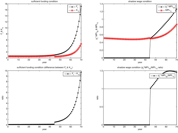
Intuitively, when the marginal product of labor in industry 2 turns positive, the su¢cient funding
condition (20) holds, which can be seen by comparing the numerator of (24) with (20). However, not
until the marginal product of labor in industry 2 become su¢ciently large such that the shadow wage
condition (24) is met, the skilled labor that is required for producing the modern good is unwilling
to work in industry 2. Thus, one may expect throughout the dynamic process of development,
time for the modern industry to be activated at which we shall say that the economy takes o¤. After
the takeo¤ (t > TW), the modern sector fully absorbs the entirety of the skilled labor and hence
complete labor specialization occurs,
L1t = Nut;
L2t+LAt = Nst:
From (20), and applying (4), (14), (15), the modern industry is more likely to be activated when
(i) the initial supply of fund (F0) is high, (ii) the initial level of modern technology (A20) is high,
(iii) the preference bias toward the traditional good ( ) is low, or (iv) the modern sector capital
barriers (q) is low. In addition, we can provide further insights toward understanding thedynamic
processof take-o¤. As time goes by, the supply of funds increases at rate St
Ft, the modern technology
increases at rate b2 = 2 1 e LAt , and the skilled labor increases at a gross growth factor
approximately:
(1 +n)
0
@1 + (1 s)e
tP1
=1 (1 e t)
1 A:
An increase in any of these rates will raise the levels of funds, modern technology and skilled labor,
thus speeding up the modernization and take-o¤ process. It may be noted that an increase in the
skilled labor growth rate not only enhances the supply of skilled workers to produce modern goods
but also improves the modern technology which in turn raises marginal products of capital and
labor in the modern industry.
4
Calibrating the Dynamic Process of Economic Development
We focus on examining the dynamic process of activating the modern industry, which requires that
the capital funds are su¢cient and that the generation-discounted cumulative shadow wage ratio
exceed one. Due to analytic complexity, we will conduct numerical exercises to compute the takeo¤
time and plotting the dynamic paths of some key variables and comparative dynamics throughout
the entire development process.
4.1 A Benchmark Case
We begin by providing a benchmark case that generally captures the development of the United
supply and the ratio of sectoral technologies to one (i.e., F1
N0 = 1 and
A10
A20 = 1). We set the initial
fraction of skilled workers about half of the current level,s= 0:2. Given that we did not have good
data on production factor shares for the actual industries, we choose to set capital’s share equal to
0:25in industry1and0:35in industry2. In the absence of a prior for the e¤ort elasticity, we choose
it as2 such that = 0:5. Similarly, there is no direct measure of modern sector capital barriers; we
simply pick a reasonable value q= 1:2, which implies a moderate degree of barriers at20%.
We calibrated, based on data from Maddison (1995), the population grew at about1:4%per year
on average over the past century, which pins down the value ofn. In the absence of a longer historic
series in U.S. sectoral outputs, we use the corresponding U.K. data from Maddison to approximate
the U.S. economy. By following the same computation as in Hansen and Prescott (2002), the
growth rates of per capita GNP for agricultural-based Malthusian and capital-intensive Solovian
technologies are1:032and 1:518, respectively. These give the respective annual rates 1 = 0:000975
and b2 = 0:0088, where the latter leads to 2 = 0:013.
We further calibrate the remaining parameters as follows: (i) the speed of knowledge
accumula-tion parameter = 0:2205and the modern technology growth parameter = 0:9722are calibrated
such that, at the time of takeo¤, the fraction of labor allocated to the modern sector is
approxi-mately40%(40:24%) and the fraction of labor allocated to the research sector is small, below0:5%
(0:28%), respectively; (ii) modern industry’s R&D productivity parameter = 347:8is chosen such
that the rate of economic growth at the takeo¤ time is about 2% (1:938%); (iii) the subjective
intergenerational discounting factor = 0:5415and the initial supply of fundF1= 0:6are such that
the saving ratio (YS) is about6%(6:33%) and the fraction of capital funds allocated to the modern
sector is about50% (52:67%), at the time of take-o¤; (iv) the initial level of modern technology is
chosen asA20= 0:7such that the modern technology at takeo¤ time is about30% (29:04%) higher
than the traditional technology; (v) the disutility scaling factorz= 0:4443is such that, at the time
of takeo¤, the disutility of e¤ort is measured (in consumption equivalence) about 10% (9:543%);
and, (vi) the preference bias parameter is set to 0:1 to produce the targeted timing of economic
takeo¤ atTW = 45. We summarize these …gures in Table 1.
The computed activation time is 45 years. Figure 3 illustrates the determination of the critical
time for the takeo¤ based on the su¢cient funding and shadow wage conditions. In the calibrated
economy, the su¢cient funding condition is met at the initial period (year 1). The shadow wage
condition is met at year45after which the modern industry is activated and the economy takes o¤.
we see discrete jumps rather than a smooth transition. The chart on real GDP, although appears
smooth, in fact indicates a jump in growth rate (the chart is in logarithmic scale). These jumps
arise because prior to the takeo¤ when the only operative sector is industry 1, the skilled labor is
treated equally as unskilled After the takeo¤, the traditional labor share continues to fall whereas
the modern labor share continues to rise. At year84 (39 years after the takeo¤), the former share
is already below the latter.6 Similar trends can be observed in the allocation of funds – the fraction
of modern industry capital rises from 1=2 to almost2=3 in 39 years. Upon activating the modern
industry, the economy also experiences a much faster rate of growth with per capita real GDP rising
sharply by about 3 times in 39 years. In addition to the reallocation of labor and capital, a key
driving force of rapid growth is endogenous technical progress: the relative TFP rises from slightly
over one at the time of takeo¤ to about1:8. The widened technology gap together with production
factor input reallocation leads to a signi…cant increase in the relative production (of modern to
traditional industries) from about 0:8 to over1:5. As a result of the increased supply, the relative
price of modern to traditional goods falls sharply.
4.2 Comparative-static Analysis
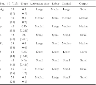
We conduct numerical comparative-static analysis with respect to the following nine parameters of
particular interest. Our results suggest that the activation time is most responsive to changes in the
initial level of the modern technology (A20), the initial level of fund supply (F1) and the subjective
discounting factor ( ) – a10%increase in each of these parameters can shorten the activation time
from the benchmark45years to26,28and24years, respectively, reducing the takeo¤ time by more
than one third. By contrast, changes in the modern industry’s R&D productivity parameter ( ) or
the education e¤ort disutility parameter (z) generate relatively small changes in activation timing.
So over the transition to a modern society, what happens to the labor shifts and capital
reallo-cation away from the traditional sector and what happens to the economy-wide aggregate output?
Our numerical results suggest that the subjective discounting factor is most in‡uential in generating
a rapid transition. In this respect, we echo Laitner (2000) who highlight saving incentives as the key
driving force for long-term economic development. Moreover, we …nd that while the preference bias
( ), the skill accumulation ( ) and the capital barrier (q) parameters are crucial for labor shifts,
their e¤ects on capital reallocation or aggregate output advancement are not nearly as important.
On the contrary, while the initial fraction of the skilled labor (s) and the initial level of fund supply
have little impact on labor shifts, they are essential for capital reallocation and aggregate output
advancement. Furthermore, concerning the initial level of the modern technology, our results
in-dicate that it is most important for capital reallocation and least in‡uential for aggregate output
advancement. Finally, as always, changes in the modern industry’s speed of growth parameter or
the education e¤ort disutility parameter have relatively little impact on factor shifts or aggregate
outputs.
One may then wonder under which circumstances the modern industry can never be activated.
In Table 2, we illustrate that a growth trap with the modern industry remaining nonoperative
throughout can arise when the initial level of the modern industry production technology (A20) is
su¢ciently low (as low as 0:5), which is consistent with the arguments by Hansen and Prescott
(2002) who emphasize the role of modern technology played in economic development. We also
…nd that activation of the modern industry may become impossible if (i) the initial funding (F1)
decreases from0:6to0:4, (ii) the altruistic factor capturing saving incentives ( ) drops from0:5415
to 0:45, (iii) the preference bias toward the traditional good ( ) increases from 0:1 to 0:2, or (iv)
the shadow cost of capital allocated to the modern industry (q) rises from 1:2to1:5, (v) the initial
size of the skill labor (s) falls from 0:2to0:1, (vi) the speed of knowledge accumulation parameter
decreases from 0:2205 to 0:15, (vii) industry 2’s R&D productivity parameter also falls from
347:8 to 100. However, the modern industry can always be activated even though the education
e¤ort disutility parameter (z) approach in…nity. The result regarding preference bias and capital
allocation barrier is consistent with the conclusion obtained by Wang and Xie (2004) in a static
framework.
In the interest of conciseness, we illustrate selectively the most representative comparative
dy-namics from the time of takeo¤ in year45 to year100(55years after the activation of the modern
industry). The three cases highlighted are the dynamic transition in response to the initial level
of modern technology, the initial fraction of the skill labor and the capital barrier measure. The
results are depicted in in Figures 5a-5c, where the paths marked with “+” (“ ”) indicates those
responding to a 10% increase (decrease) in one of the three exogenous parameters. While labor,
capital and production all shift rapidly in response to such an increase in the initial level of modern
technology, the resultant shifts in response to the initial fraction of skilled labor are more moderate.
from traditional to modern sectors, though changes in the relative output are more moderate over
the transition. As a result of the aforementioned transition processes, the per capita real income
grow at the highest rate in response to the initial level of modern technology and the lowest in
response to the initial fraction of skilled labor.
4.3 Policy Implications
Our …ndings yield several useful policy implications. Speci…cally, the results suggest that there are
many ways for the government to help activating a modern industry and enabling an economy to
take o¤. Such public policies include at least (i) government subsidies to create su¢cient incentives
for industrial transformation, (ii) establishment of public enterprises in early development when
modern industries are not pro…table, and (iii) direct technology transfer or imitation to jump-start
the modern industry. For example, should the government fully internalize capital externalities
originated in the modern sector by ways of investment subsidy or public enterprising, the scale
barrier can be completely removed. In this case, our numerical results suggest that the activation
time is reduced all the way to zero and the economy can take o¤ immediately.
To the end, it is useful to discuss plausible sets of parameters that may replicate the speed of
take-o¤ experienced by the UK, Canada, Korea and Taiwan. As documented by Gollin, Parente
and Rogerson (2002), it took about 55 years for the UK to double its per capita real income from
2;000(1990 US$) to4;000, while it only took about 32,15 and 10 years, respectively, for Canada,
Korea and Taiwan to do so. For illustrative purposes, let us use these …gures to capture the take-o¤
time in our model. We can obtain the take-o¤ time of 55 years as in the UK with lower initial
levels of the modern technology and funding, a lower subjective discounting factor and a higher
shadow cost associated with modern capital (A20= 0:69; F1 = 0:59; = 0:53andq= 1:23). On the
contrary, the take-o¤ time of32for Canada can be captured with higher initial levels of the modern
technology and funding, a higher subjective discounting factor and a lower shadow cost associated
with modern capital (A20 = 0:715; F1 = 0:61; = 0:55 and q = 1:19). With a slightly better
initial condition (A20 = 0:75 and F1 = 0:65) while maintaining = 0:55 and q = 1:19, the take-o¤
time becomes15years, thereby mimicking the cases of Korea. Similarly, with a much better initial
condition (A20 = 0:77 and F1 = 0:66) while maintaining = 0:55 and q = 1:19, the take-o¤ time
becomes10years, thereby mimicking the cases of Taiwan. In the case of Taiwan, the government has
undertaken a series of education reforms and established public programs by subsidizing investment
providing funding to the private sector using foreign aid and monopoly revenues.
5
Concluding Remarks
By constructing a dynamic general equilibrium model with endogenous activation of the modern
industry, we have identi…ed an array of preference, technology, funds and labor skill forces to
en-able the take-o¤ of a closed economy. By calibrating the model to …t historic U.S. development, our
quantitative results suggest that the timing of economic takeo¤ depends most crucially on the initial
levels of the modern technology and fund supply as well as the subjective intergenerational
discount-ing factor. While individual’s savdiscount-ing incentives is most important for the speed of modernization,
the preference bias, the skill accumulation and the capital allocation barrier are in‡uential for labor
reallocation, and the initial states of skills, funds and modern technologies are crucial for capital
reallocation. Along the dynamic transition path, labor, capital and output are most responsive to
the initial state of modern technologies but least responsive to the initial state of skills.
In order to accomplish our analysis, we have imposed a number of simplifying assumptions
that help the tractability of our model framework. It is therefore natural to relax some of these
assumptions by further simplifying other parts of the model structure to check the robustness
of our main conclusions. For example, in the aspects of the dynamic take-o¤ theory, one may
endogenize capital accumulation process based on intertemporal consumption-savings trade-o¤ as
in the standard Ramsey optimal growth framework, or endogenize the knowledge accumulation
process based on learning-by-doing (as in Lucas 1993). Since trade is believed to play a major role
in many newly industrialized economies, one may also extend the model to a small open economy
case (as in Bond, Jones and Wang, 2005 or as in Trindade, 2005) to understand how globalization
may help advance an economy and to whether tari¤ reduction, export learning or foreign direct
References
[1] Acemoglu, D., Guerrieri, V., 2008. Capital deepening and nonbalanced economic growth.
Jour-nal of Political Economy 116, 467–498.
[2] Aghion, P., 2002. Schumpeterian growth theory and the dynamics of income inequality.
Econo-metrica 70, 855–882.
[3] Aghion, P., Bolton, P., 1997. A theory of trickle-down growth and development. Review of
Economic Studies 64, 151–172.
[4] Autor, D.H., Katz, L.F., Krueger, A.B., 1998. Computing inequality: Have computer changed
the labor market? Quarterly Journal of Economics 113, 1169–1213.
[5] Benhabib, J., Farmer, R.E.A., 1994. Indeterminacy and increasing returns. Journal of
Eco-nomic Theory 63, 19–41.
[6] Bond, E.W., Jones, R., Wang, P., 2005. Economic take-o¤s in a dynamic process of
globaliza-tion.Review of International Economics 13, 1–19.
[7] Bond, E.W., Trask, K., Wang, P., 2003. Factor accumulation and trade: Dynamic comparative
advantage with endogenous physical and human capitals. International Economic Review 44,
1041–1060.
[8] Fei, J.C.H., Ranis, G., 1964.Development of the Labor Surplus Economy: Theory and Policy.
Homewood, Illinois, Richard D. Irwin for the Economic Growth Center, Yale University.
[9] Fei, J.C.H., Ranis, G., 1997.Growth and Development from an Evolutionary Perspective.
Black-well, Cambridge, MA.
[10] Gollin, D., Parente, S., Rogerson, R., 2002. The role of agriculture in development. American
Economic Review, Papers and Proceedings 92, 160–164.
[11] Goodfriend, M., McDermott, J., 1995. Early development. American Economic Review 85,
116–133.
[12] Hansen, G.D., Prescott, E.C., 2002. Malthus to Solow. American Economic Review 92, 1205–
1217.
[13] Kongsamut, P., Rebelo, S., Xie, D., 2001. Beyond balanced growth.Review of Economic Studies
[14] Laitner, J., 2000. Structural change and economic growth. Review of Economic Studies 67,
545–561.
[15] Lewis, W.A., 1955. The Theory of Economic Growth. Allen and Urwin, London, UK.
[16] Lucas, R.E. Jr., 1988. On the mechanics of economic development.Journal of Monetary
Eco-nomics 22, 3–42.
[17] Lucas, R.E. Jr., 1993. Making miracle. Econometrica 61, 251–272.
[18] Lucas, R.E. Jr., 2004. Life earnings and rural-urban migration. Journal of Political Economy
112, S29–S59.
[19] Maddison, A., 1995. Monitoring the World Economy 1820-1992. OECD Press, Paris, France.
[20] Ngai, L.R., 2004. Barriers and the transition to modern growth.Journal of Monetary Economics
51, 1353–1383.
[21] Ngai, L.R., Pissarides, C.A., 2007. Structural change in a multisector model of growth.
Amer-ican Economic Review 97, 429-443.
[22] Romer, P., 1986. Increasing returns and long-run growth. Journal of Political Economy 94,
1002–1037.
[23] Rosenstein-Rodan, P.N., 1961.Notes on the theory of the ‘Big Push’. in Howard S. Ellis (ed.),
Economic Development for Latin America. Macmillan, London, UK, 57–66.
[24] Rostow, W.W., 1960.The Stage of Economic Growth. Cambridge University Press, Cambridge,
UK.
[25] Saint-Paul, G., Verdier, T., 1993. Education, democracy and growth. Journal of Development
Economics 42, 399–407.
[26] Trindade, V., 2005. The big push, industrialization and international trade: The role of exports.
Journal of Development Economics 78, 22–48.
[27] Tsiang, S.C., 1964. A model of economic growth in Rostovian stages.Econometrica32, 619–648.
[28] Tung, A., Wan, H.Y., 2008. Industry activation: A study of its micro-foundations. Mimeo,
Cornell University, Ithaca, NY.
[29] Wang, P., Xie, D., 2004. Activation of a modern industry. Journal of Development Economics
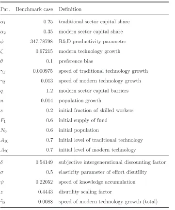
Table 1: Parameters for numerical analysis
Par. Benchmark case Definition
α1 0.25 traditional sector capital share
α2 0.35 modern sector capital share
φ 347.78798 R&D productivity parameter
ζ 0.97215 modern technology growth
θ 0.1 preference bias
γ1 0.000975 speed of traditional technology growth
γ2 0.013 speed of modern technology growth
q 1.2 modern sector capital barriers
n 0.014 population growth
s 0.2 initial fraction of skilled workers
F1 0.6 initial supply of fund
N0 0.6 initial population
A10 0.7 initial level of traditional technology
A20 0.7 initial level of modern technology
δ 0.54149 subjective intergenerational discounting factor
σ 0.5 elasticity parameter of effort disutility
ψ 0.22052 speed of knowledge accumulation
z 0.4443 disutility scaling factor
b
γ2 0.0088 speed of modern technology growth (total)
Table 2: Activation time, growth traps and comparative static adjustments
Comparative statics
Size of responses to 10% increase in each parameter
Par. +(−)10% Traps Activation time Labor Capital Output
A20 26 0.5 Large Median Large Small
(57) [0.7]
s 40 0.1 Median Small Median Median
(50) [0.2]
ψ 40 0.15 Median Large Median Median
(53) [0.221]
φ 42 100 Small Small Small Small
(48) [347.8]
F1 28 0.4 Large Small Median Median
(55) [0.6]
δ 24 0.45 Large Large Large Large
(63) [0.541]
z 46 N/A Small Small Small Small
(43) [0.444]
q 56 1.5 Median Large Small Small
(25) [1.2]
θ 54 0.2 Median Large Small Small
(26) [0.1]
Notes: The activation time,TW ≡min{t|Ω(L2t)≥1}. TW for benchmark case is 45. TW = 62 asz→ ∞. 10%
MB
or MC
1
MC
0 MC
Y2t or !
MB
[image:24.612.177.429.80.293.2]!t
Figure 1: Consumption-saving choice condition
MB
orMC
1
MC
0
MC z
Y2t or
s, ,Y1t!
0
MB
1
MB
!t
[image:24.612.174.426.406.611.2]0 10 20 30 40 50 60 70 0 2 4 6 8 10 12 14 16 18
sufficient funding condition
year Ft & K 1t Ft K 1t
0 10 20 30 40 50 60 70
0 0.2 0.4 0.6 0.8 1 1.2 1.4
shadow wage condition
year p t * MPL 2t & MPL 1t
pt* MPL2t
MPL 1t
0 10 20 30 40 50 60 70
0 1 2 3 4 5 6 7 8 9 10
sufficient funding condition (difference between F t & K1t)
year
ratio
F t − K1t
0 10 20 30 40 50 60 70
0 0.5 1 1.5
shadow wage condition (p
t*MPL2t/MPL1t ratio)
year
ratio
p
[image:25.792.142.719.76.508.2]0 20 40 60 80 100 0 0.1 0.2 0.3 0.4 0.5 0.6 0.7 0.8 0.9 1
sectoral labor allocation
year
ratio
L
2t/Nt
L
1t/Nt
0 20 40 60 80 100
0 0.001 0.002 0.003 0.004 0.005 0.006 0.007 0.008 0.009 0.01
R&D labor allocation
year
index
L
At/Nt
0 20 40 60 80 100
0 0.1 0.2 0.3 0.4 0.5 0.6 0.7
fraction of capital in industry 2
year
ratio
q*K2t/Ft
0 20 40 60 80 100
0.8 1 1.2 1.4 1.6 1.8 2 2.2
TFP ratio between modern and traditional sectors
year
index
A
2t/A1t
10 20 30 40 50 60 70 80 90 100
−0.5 0 0.5 1 1.5 2 2.5 relative price year index pt
0 20 40 60 80 100
0 0.2 0.4 0.6 0.8 1 1.2 1.4 1.6
relative production between two industries
year
index
pt*Y2t/Y1t
0 20 40 60 80 100
−1 −0.5 0 0.5 1 1.5 2 2.5 3
real GDP and real GDP per capita
year
index
ln(Y
t)
ln(Y
t/Nt)
0 20 40 60 80 100
0 0.05 0.1 0.15 0.2 0.25 0.3 0.35 0.4
endogenous rate of saving
year
ratio
[image:26.612.103.508.27.664.2]ρt
0 20 40 60 80 100 0 0.1 0.2 0.3 0.4 0.5 0.6 0.7 0.8 0.9 1
sectoral labor allocation
year
ratio
L2t/Nt
L1t/Nt
+L 2t/Nt +L
1t/Nt
0 20 40 60 80 100
0 0.1 0.2 0.3 0.4 0.5 0.6 0.7
fraction of capital in industry 2
q*K2t/Ft
+q*K 2t/Ft
0 20 40 60 80 100
−0.5 0 0.5 1 1.5 2 2.5 3 year index
real GDP per capita
ln(Yt/Nt)
+ln(Yt/Nt)
0 20 40 60 80 100
0 0.2 0.4 0.6 0.8 1 1.2 1.4 1.6
relative production between two industries
year
index
pt*Y2t/Y1t
[image:27.792.138.719.74.506.2]0 20 40 60 80 100 0 0.1 0.2 0.3 0.4 0.5 0.6 0.7 0.8 0.9 1
sectoral labor allocation
L2t/Nt
L1t/Nt
+L 2t/Nt +L
1t/Nt
0 20 40 60 80 100
0 0.1 0.2 0.3 0.4 0.5 0.6 0.7
fraction of capital in industry 2
year
ratio
q*K 2t/Ft
+q*K2t/Ft
0 20 40 60 80 100
−0.5 0 0.5 1 1.5 2 2.5 year index
real GDP per capita
ln(Y t/Nt) +ln(Y
t/Nt)
0 20 40 60 80 100
0 0.2 0.4 0.6 0.8 1 1.2 1.4 1.6
relative production between two industries
year
index
p t*Y2t/Y1t
[image:28.792.143.722.70.507.2]+pt*Y2t/Y1t
0 20 40 60 80 100 0 0.1 0.2 0.3 0.4 0.5 0.6 0.7 0.8 0.9 1
sectoral labor allocation
L2t/Nt
L1t/Nt
−L 2t/Nt −L
1t/Nt
0 20 40 60 80 100
0 0.1 0.2 0.3 0.4 0.5 0.6 0.7
fraction of capital in industry 2
year
ratio
q*K2t/Ft
−q*K 2t/Ft
0 20 40 60 80 100
−0.5 0 0.5 1 1.5 2 2.5 3 year index
real GDP per capita
ln(Y t/Nt) −ln(Y
t/Nt)
0 20 40 60 80 100
0 0.2 0.4 0.6 0.8 1 1.2 1.4 1.6 year index
relative production between two industries
p t*Y2t/Y1t −p
[image:29.792.143.719.75.507.2]