Munich Personal RePEc Archive
Credit Constraints, Quality, and Export
Prices: Theory and Evidence from China
Fan, Haichao and Lai, Edwin L.-C. and Li, Yao Amber
The Hong Kong University of Science and Technology
1 August 2012
Online at
https://mpra.ub.uni-muenchen.de/52316/
Credit Constraints, Quality, and Export Prices:
Theory and Evidence from China
∗
Haichao Fan
†SHUFE
Edwin L.-C. Lai
‡HKUST
Yao Amber Li
§HKUST This Version: December 2013
First Draft: February 2012
Abstract
This paper examines the relationship between the credit constraints faced by a firm and the unit value prices of its exports. The paper modifiesMelitz’s (2003) model of trade with heterogeneous firms by introducing endogenous quality and credit constraints. The model predicts that tighter credit constraints faced by a firm reduce its optimal prices as its choice of lower-quality products dominates the price distortion effect resulting from credit constraints under the endogenous quality case. However, when endogenous quality choice is not possible under the exogenous quality case, there is an opposite prediction that prices increase as firms face tighter credit constraints. An empirical analysis using Chinese bank loans data, Chinese firm-level data from the National Bureau of Statistics of China (NBSC), and Chinese customs data strongly supports the predictions of the endogenous quality case and confirms the mechanism of quality adjustment: firms optimally choose to produce lower-quality products when facing tighter credit constraints. Moreover, the predictions of the exogenous quality case are supported by using quality-adjusted prices in regression analysis and by using quality variation across firms within the same product.
JEL: F1, F3, D2, G2, L1
Keywords: credit constraints, credit access, credit needs, quality, endogenous quality, export prices, heterogeneous firms, productivity
∗We thank Gene Grossman, Robert Staiger, Shang-Jin Wei, Stephen Yeaple, Kalina Manova, Mark Roberts, Norman Loayza, Davin Chor, Jonathan Vogel, Jim MacGee, Heiwai Tang, Loretta Fung, Yi Lu, Kenneth Corts, Pengfei Wang, David Cook, Albert Park, Xi Li, Nelson Mark, Zhigang Tao, Larry Qiu, Wen Zhou, Zhanar Akhmetova, Wei Liao, Peng Wang, the participants of the Midwest International Trade Conference (Indiana University Bloomington, May 2012), the Asia Pacific Trade Seminars Annual Meeting (Singapore Management University, July 2012), the Workshop on Emerging Economies (University of New South Wales, August 2012), the 2nd China Trade Research Group Annual Conference (Shandong University, China, May 2012), the 7th Biennial Conference of Hong Kong Economic Association (Lingnan University, HK, December 2012), and of seminars held at HKUST, University of Hong Kong, University of Western Ontario, Hong Kong Institute for Monetary Research, Shanghai University of Finance and Economics, Fudan University, Shanghai Jiaotong University, Zhejiang University, and Lingnan College at Sun Yat-sen University for helpful discussions. All remaining errors are our own.
†Fan: School of International Business Administration, Shanghai University of Finance & Economics. Email: fan.haichao@mail.shufe.edu.cn.
‡Lai: Department of Economics, The Hong Kong University of Science and Technology. Email: elai@ust.hk. CESifo Research Network Fellow.
§Li: Corresponding author. Department of Economics and Faculty Associate of the Institute for Emerging Market Studies (IEMS), Hong Kong University of Science and Technology, Clear Water Bay, Kowloon, Hong Kong SAR-PRC. Email: yaoli@ust.hk. URL:ihome.ust.hk/∼yaoli. Tel: (852)2358 7605; Fax: (852)2358 2084. Research Affiliate of the
1
Introduction
There is a growing body of literature on the effects of credit constraints on international trade, es-pecially after the financial crisis of 2008. Most prior studies have focused on either explaining the
mechanism of why exporters need more credit than domestic producers (e.g., Amiti and Weinstein,
2011; Feenstra et al.,forthcoming), or the consequences of different credit conditions on export per-formance, comparative advantage, multinational activities and spillovers.1 However, to the best of our
knowledge, the impacts of credit constraints on a firm’s choice of optimal quality and optimal price have not been explored. This paper fills a gap in the literature by linking credit constraints to firm
attributes and action such as its productivity and its choice of product quality and optimal prices.
Understanding the mechanism through which credit constraints affect export prices helps us better
understand how credit constraints affect a firm’s exporting behavior via optimal choice of quality and pricing. In particular, it helps to explain the differential impacts of credit constraints on the intensive
margin of trade across products through their effects on the unit value prices of different products. As the intensive margin of a product is measured by the total value of its exports, the change in
the intensive margin is affected by two factors: the change in the quantity exported, and the change in the unit value price of the exported product. Therefore, a thorough analysis on the effect of credit constraints on unit value prices can help us better understand their effect on the intensive
margin of trade. Moreover, credit constraints affect bank loans to firms, which are used to cover upfront costs. Tighter credit constraints would affect upfront costs and therefore distort a firm’s
choice of optimal price more than before. As noted in the literature on financial distress, binding credit constraints may cause firms to act in ways that would be suboptimal in normal times, which may lead them to produce lower-quality products, which in turn lowers the unit value price of the
product (Phillips and Sertsios, 2011). However, how and why credit constraints affect the export prices of different products differently has not been studied thoroughly. Our paper tries to fill this
gap in the literature.
To study the impacts of credit constraints on export prices, we build a heterogenous-firm trade model with endogenous quality and credit constraints. The introduction of credit constraints acts through two channels. First, we assume that firms must externally finance a certain fraction of its
total costs in order to produce as well as to enter foreign markets. This fraction captures the credit needs of the firm. The higher is this fraction, the more likely the firm faces binding credit constraints. Second, we assume that due to frictions in the financial markets, a firm cannot borrow more than a certain fraction of its expected cash flow. This fraction of a firm’s expected cash flow capture the firm’scredit access. To sum up, a firm is more likely to have tighter credit constraints if it has a higher level of “credit needs” or faces a lower level of “credit access”.
1See Manova (2013), Manova et al. (2011), Chor and Manova(2012), Minetti and Zhu(2011), Ju and Wei (2011),
The theory indicates that the impacts of credit constraints on prices depend on two opposing forces: (i)the quality adjustment effect, which lowers product quality and therefore reduces prices when credit constraints are more stringent; (ii)the price distortion effect, which increases price when credit constraints are tighter. The intuition behind the price distortion effect is as follows. Given product quality, a firm facing tighter credit constraints will reduce its output, leading to excess demand for
its product at the initial price level, which in turn pushes up its price. We call this effect the price distortion effect. When product quality is endogenously chosen by a firm and there is a large scope
for quality variation, the quality adjustment effect dominates the price distortion effect, and therefore optimal prices fall when firms face tighter credit constraints. On the contrary, when the endogenous quality choice is not allowed, the theory predicts the opposite outcome: the existence of more stringent
credit constraints wouldraiseoptimal prices. Meanwhile, the relationship between export prices and firm productivity also depends on whether the quality is an endogenous choice by the firm: prices
increase in productivity under the endogenous quality case while decrease in productivity under the exogenous quality case.
Next, we test our model using a matched Chinese firm-product level dataset, based on Chinese firm-level production data from the National Bureau of Statistics of China (NBSC) and Chinese
customs data at the transaction-product level. The unique advantage of this matched database is that it contains information on unit value prices of exports at the product-firm level as well as the
information needed to measure credit constraints and firm productivity. To measure the severity of credit constraints via credit needs faced by firms, we first followManova et al. (2011) to employ four different measures at the industry level: external finance dependence, R&D intensity,
inventory-to-sales ratio, and asset tangibility. We use US data for those measures in our main regressions because the US financial markets are mature and they could reflect true credit needs by industry. Also the
measures based on US data have been widely used in cross-country studies in the literature. For robustness, we also followRajan and Zingales(1998) andManova(2013) to calculate external finance
dependence using Chinese firm-level data. To proxy for credit access, we collect balances of bank credits, long-term bank loans and short-term bank loans by province (normalized by province GDP) in China to reflect the credit access by firms located in different regions. In addition, we compare
different types of firm ownership in China as each type is expected to be associated with a different level of credit access. Finally, to compute productivity, we use the augmented Olley and Pakes’s
(1996) approach, which alleviates simultaneity bias and selection bias, to estimate a firm’s total factor productivity. In the robustness checks, we also report results with labor productivity measured by the value added per employee and the results with the TFP computed by the augmentedAckerberg et al.’s
(2006) approaches.
We test the empirical implications of our model and the results strongly support the theoretical predictions of the endogenous quality case: First, tighter credit constraints (i.e., either a higher level of
when a firm faces more stringent credit constraints, it produces lower-quality products. Third, there is a positive relationship between export prices and firm productivity. Our results are robust to various
specifications, including the estimations with different fixed effects and clustering at different levels.
We also verify the quality-adjustment mechanism and test the exogenous-quality case through
two exercises. First, we estimate quality and quality-adjusted prices by adopting Khandelwal et al.’s (forthcoming) method, in which quality-adjusted price is defined as observed price less estimated
qual-ity. We then replicate the baseline regressions with estimated quality and quality-adjusted prices as dependent variable. When we regress quality-adjusted prices, the results are consistent with the pre-dictions of the exogenous quality case: tighter credit constraints raise export prices; more productive
firms set lower prices; the positive effects of credit access on prices are attenuated, and, sometimes, become significantly negative. Second, we compare the results based on a set of products with higher
variation in product quality and those based on another set of products with lower variation in prod-uct quality. We find that firms producing prodprod-ucts associated with higher quality variation are more
affected by credit constraints and the observed product prices are more in line with the predictions of the endogenous quality case. In other words, the magnitudes of the predicted effects of credit constraints on prices are larger for the observations with more variation of quality, thus validating the
mechanism of quality adjustment.
The main contribution of this paper is that it presents theory and evidence from highly disag-gregated Chinese data that tighter credit constraints induce firms to lower the quality of products they export and thus reduce export prices. This contributes to the emerging literature on the role
of financial constraints in international trade. To the best of our knowledge, this paper provides the first compelling analysis of the impacts of credit constraints on export prices under a
heterogeneous-firm framework. This paper also complements the large quality-and-trade literature in conheterogeneous-firming the prevalence of product quality heterogeneity at the firm level and explaining the mechanism of
quality adjustment. Our finding of a positive relationship between export prices and firm produc-tivity is consistent with the findings in the literature on product quality (e.g., Verhoogen, 2008;
Kugler and Verhoogen,2012;Hallak,2010;Johnson,2012; andHallak and Sivadasan,2011).
The remainder of the paper is organized as follows. Section 2 presents a trade model with
het-erogeneous firms, featuring endogenous product quality and credit constraints to illustrate the impact of credit constraints on the optimal prices of exports. Section 3 describes the data and introduces the strategy of the empirical analysis. Section 4 presents the empirical results and Section 5 provides
some robustness checks. The final section concludes.
2
A Model of Credit Constraints, Quality, and Export Prices
heterogeneous-firm trade model of Melitz (2003), by incorporating endogenous quality and credit constraints in the analysis. Goods are differentiated, and each good is produced by one firm. The
main departure from the existing literature is that firms are heterogeneous in both their productivity and the degree of credit constraints they face. Firms choose not only the optimal price but also the optimal product quality.
2.1 Preferences and the Market Structure
We denote the source country by iand the destination country by j, wherei, j ∈1, . . . , N. Country
j is populated by a continuum of consumers of measure Lj. Consumers in country j have access to
a set of goods Ωj, which is potentially different across countries. In each source country i, there is
a continuum of firms that ex ante differ in their productivity level, φ, the degree of credit access,
θ, and the credit needs, d. A firm facing higher θ has more credit access; a firm with higher d has greater credit needs. A lower level ofθor a higher level of dimplies tighter credit constraints for this firm (see Section 2.2for more detail). We assume that a representative consumer in country j has a constant-elasticity-of-substitution (CES) utility function given by:
Uj =
Z
ω∈Ωj
[qij(ω)xij(ω)]
σ−1
σ dω
! σ σ−1
where qij(ω) is the quality of variety ω originated from country i; xij(ω) is country j’s quantity
consumed of variety ω originated from country i; and σ >1 is the elasticity of substitution between varieties. Therefore, consumer optimization yields the following demand function for variety ω:
xij(ω) = [qij(ω)]σ−1
[pij(ω)]
−σ
P1−σ j
Yj (1)
where pij(ω) is the price of variety ω, Pj =
R
ω∈Ωj[pij(ω)/qij(ω)]
1−σ
dω
1 1−σ
is an aggregate price index (adjusted by the demand shifter), andYj represents the total expenditure of country j. Given
the same price, higher-quality products generate a larger demand.
2.2 The Firm’s Problem
A firm’s technology is captured by a cost function that features, for any given quality, a constant
marginal cost with a fixed overhead cost. Labor is the only factor of production. Following convention, we assume that there is an iceberg trade cost such that τij ≥1 units of good must be shipped from
countryiin order for one unit to arrive in j. Firms face no trade costs in selling in its home market, i.e., τii = 1. To simplify notation, the subscripts for source and destination as well as the index for
variety are suppressed hereafter. In addition, the wage rate of the source country is normalized to
We assume that there is a positive relationship between quality and marginal cost of production. The rationale is that a higher marginal cost is required to produce a higher-quality product. The
positive relationship between quality and marginal cost is common to the recent quality-and-trade literature, for instance, Verhoogen (2008) and Johnson (2012). In this paper, the marginal cost of production is assumed to beqα/φ, whereα∈(0,1). Hence, the marginal cost increases in quality q,
and α captures the elasticity of marginal cost with respect to quality.
Except for variable cost, firms face fixed cost in producing and exporting goods,f qβ(β > 0), where
f is a constant and 1/β measures the effectiveness of fixed investment in raising quality. The fixed cost represents the fixed investments in production and export associated with quality improvement
(e.g., costs of employing higher-quality inputs, R&D expenditures to improve the product quality, or the changes in modes of international shipping from ocean freight to air freight, etc.).2
We posit that all firms are subject to possible liquidity constraints in paying all types of costs. Like the extended model inManova(2013), we assume that exporters need to raise outside capital for
a fraction d∈(0,1) of all costs associated with foreign sales, including variable costs and fixed costs mentioned above.3 This fraction d represents thefinancial needs of a firm. The higher the financial
needs, the higher isd, and we call this fractiondthe “credit needs” parameter. We also assume that, constrained by the level of financial development, firms cannot borrow more than a fraction θ of the expected cash flow from exporting. Ifθis higher, firms can borrow more from external finance (mainly through bank loans). Therefore,θ is referred to as thecredit access by firms. A higher level ofcredit needs d or a lower level of credit access θ implies that firms are more likely to face tighter credit constraints. Consequently, the optimization problem of a firm with productivity φ, credit access θ, and credit needsdis given by:4
max
p,q
p− τ q
α
φ
qσ−1 p−σ
P1−σY −f q
β (2)
s.t. θ
p−(1−d)τ q
α
φ
qσ−1 p −σ
P1−σY −(1−d)f q β
(3)
≥d
τ qα φ q
σ−1 p−σ
P1−σY +f q β
where budget constraint (3) can be viewed as the “cash flow constraint” condition, in the same spirit as Manova (2013) and Feenstra et al. (forthcoming). Solving this optimization problem by choosing
2In this paper we only consider exporting firms.
3We also consider the case when only fixed costs are financed by outside capital in Appendix (see AppendixC), and
this change in the model’s set-up does not alter the main predictions of our model.
4For simplicity of notation, we suppress variety ω and subscripts of country (i, j). It should be also pointed out
pricep and quality q yields
p= σ
σ−1
1 +d(1−θ)λ θ(1 +λ)
τ qα
φ (4)
qσ−1p1−σ
P1−σY =
σβ
(1−α) (σ−1)
1 +d(1−θ)λ θ(1 +λ)
f qβ (5)
whereλis the Lagrangian multiplier associated with the budget constraint condition (3) (see Appendix
A for the detailed derivation of first-order conditions).
The budget constraint (3), together with conditions (4) and (5), yield:
σβ
(1−α) (σ−1)
1 +d(1−θ)λ θ(1 +λ)
≥
1−d+d
θ
β
1−α + 1
(6)
Given credit needsd, there exists a cutoff level of credit accessθhsuch that budget constraint (3) is
binding if and only ifθ < θh.5 Likewise, given credit accessθ, there exists a cutoff level of credit needs
above which the budget constraint (3) is binding. Next, we analyze two cases according to whether
budget constraint (3) is binding.
Case 1: The budget constraint (3) is binding, i.e.,θ < θh.
Let ∆ ≡
1 +d(1θ(1+−θ)λλ), which reflects the price distortion based on equation (4).
Accord-ing to equation (6), we obtain the expression for ∆ after eliminating λ: ∆ ≡
1 +d(1θ(1+−θ)λλ) =
1−d+dθ σ−1
σ 1 + 1
−α β
. Therefore, ∆ is only related to credit access θ and credit needs d. In other words, credit access θ and credit needs d form a sufficient statistic for the price distortion. We call this effect theprice distortion effect. It is obvious that the extent to which price is distorted is related to credit access θand credit needs d. Lower credit access θor higher credit needs dincreases the price distortion caused by the binding budget constraint. The intuition behind the price
distor-tion effect is as follows. Given product quality, a firm facing tighter credit constraints will reduce its output, leading to excess demand for its product at the initial price level, which in turn pushes up its
price.
Now, equations (3) and (4) imply that the optimal quality chosen by firms satisfies the following condition:
qβ−(1−α)(σ−1) = (1−α) (σ−1)
σβf ∆
−σ
σ σ−1
τ φ
1−σ
Y
P1−σ (7)
Define condition (i) asβ >(1−α) (σ−1). Under condition (i), there is a positive correlation between firm productivity φ and quality q, given credit access θ and credit needs d. This suggests that more productive firms choose higher quality, which is consistent with the findings of the quality-and-trade
literature. Condition (i) ensures the existence of the optimal quality. Otherwise, ifβ is too small, it
5Equation (6) implies that budget constraint (3) is binding if and only ifθ < θ
implies that the firm could easily improve quality without incurring large fixed cost (recall that f qβ
represents the fixed cost), and then the firm would choose quality q to be infinite.
Given firm productivity, condition (i) also ensures that a firm with more credit access or less credit needs chooses higher optimal quality. This is because equation (7) tells us that, given productivity,
an increase in θ or a reduction in d (i.e., more credit access or lower credit needs) relaxes the firm’s credit constraints through the change in ∆, and therefore induces the firm to choose a higher optimal
quality q, which in turn leads to a higher price set by the firm. We call this mechanism the quality adjustment effect.
Hence, the optimal pricing rule (4), together with (7), yield:
p=
(1−α) (σ−1)
σβf
Ψ ∆1−σΨ
σ σ−1
τ φ
1+(1−σ)Ψ Y
P1−σ
Ψ
(8)
where Ψ = α
β−(1−α)(σ−1) > 0. Define Condition (ii) as β < (σ −1). If Condition (ii) holds (in addition to Condition (i) ), then a firm’s optimal price is positively correlated with firm productivity as conditions (i) and (ii) together imply that 1 + (1−σ) Ψ<0. The condition (ii) ensures that β is not too large. Ifβ is too large, it would be difficult for the firm to adjust quality and to choose higher-quality product as the elasticity of fixed cost with respect to higher-quality is high: a small improvement in quality would incur a large increase in fixed cost. Therefore, a very large β is equivalent to the case that the firm cannot flexibly choose optimal quality, and thus quality variance is small. Under this case, the price distortion effect would dominate the quality adjustment effect, and this would
generate the same prediction as in an exogenous-quality model, i.e., a model where endogenous quality choice is not allowed. In this paper, our focus is endogenous quality choice but we will also
compare the implications of both endogenous and exogenous quality in the end of this section.
Let us define condition (A) as β1 > σ−11 > 1−α
β . Condition (i) and (ii) combined is equivalent
to condition (A). When condition (A) holds, a firm with higher productivity charges higher optimal prices. The intuition behind this positive correlation between firm productivity and export prices is
due to two opposing forces: the quality adjustment effect (i.e., higher-productivity firms set higher prices via selling higher-quality products) and the productivity effect (i.e., higher-productivity firms are able to charge lower prices via having lower marginal cost for any given quality). When the quality
adjustment effect dominates the productivity effect, there exists a positive relationship between firm productivity and export prices.
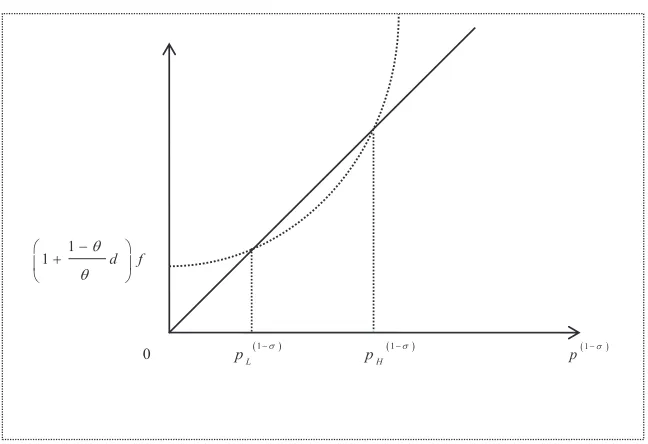
Under condition (A), 1−σΨ < 0 is also satisfied. Hence, tighter credit constraints (via either higher credit needs d or lower credit access θ) eventually reduce the optimal price. This implies that the quality adjustment effect dominates the price distortion effect. Here, the impact of credit constraint on export prices also depends on two opposing forces: One is caused by the price distortion
Figure 1: The relationship between prices, TFP, and credit constraints
log(TFP)
Tighter credit constraints:
(higher credit needs d and/or lower credit access q )
0
Endogenous Quality log(Price)
log(Price) Exogenous Quality
log(TFP)
increase the optimal price when a firm faces higher credit needsdand lower credit accessθ(i.e., when
dincreases or θ decreases, the price distortion ∆ increases and therefore price increases according to equation (4)). However, the latter effect tends to reduce the optimal price when a firm faces tighter credit constraints. This is because tighter credit constraints induce ∆ to increase, and hence induce
firms to produce a lower-quality product according to equation (7), which in turn lowers optimal price according to equation (4). Under condition (A), the quality adjustment effect dominates, and
therefore, firms facing tighter credit constraints set lower prices. The graph in the left panel of Figure
1 illustrates the relationship between (log) price, (log) TFP, and credit constraints when condition (A) holds under Case 1: the solid line corresponds to more relaxed credit constraint (i.e., a higher θ
and a lowerd), and the dashed line captures the tighter credit constraint situation (i.e., a lowerθ and a higher d).
Case 2: The budget constraint (3) is nonbinding, i.e.,θ > θh.
Equations (4) and (5) imply:
qβ−(1−α)(σ−1) = (1−α) (σ−1)
σβf
σ σ−1
τ φ
1−σ
Y
P1−σ (9)
together with (4), imply that the optimal pricing rule is given by
p=
(1−α) (σ−1)
σβf
Ψ
σ σ−1
τ φ
1+(1−σ)Ψ
Y P1−σ
Ψ
(10)
When condition (A) holds, then 1 + (1−σ)Ψ<0, and so equation (10) implies that there is a positive relationship between price and productivity. Therefore, the solid line in the left panel of Figure 1
still describes the relationship between (log) price and (log) TFP. However, the optimal prices are
not affected by credit access θ or credit needs d anymore, as firms have sufficient credit access (i.e.,
θ > θh). Therefore, the solid line in the left panel of Figure1does not shift asθ or dchanges.
2.3 Predictions
In the rest of this paper, we will concentrate on the central case when Case 1 and Condition (A) both
hold. These parameter conditions are supported by empirical evidence. For example, based on the data of Chinese exporting firms, Manova and Zhang (2012) propose that more successful exporters with
higher export revenue or larger export scope produce higher quality goods and charge higher export prices, implying that the parameter restrictions given by condition (A) tend to hold for Chinese data.
Ge et al. (2012) also find that more productive firms charge higher export prices using Chinese firm data. Later, our empirical results also confirm this point. Henceforth, unless otherwise noted, we focus on Case 1 when Condition (A) holds. Therefore, we have the following testable propositions:
Proposition 1. Given firm productivity, tighter credit constraints resulting from either lower level of credit access (i.e., a lower θ) or from higher credit needs (i.e., a higher d) reduce the optimal export price set by a firm. In this case, export prices increase with productivity, ceteris paribus.
Proposition 2. (Quality Adjustment Effect): Given productivity, tighter credit constraints (i.e., higher dor lower θ) lower the optimal product quality chosen by a firm.
Propositions1and2are based on the assumption that quality is endogenously chosen by firms and
therefore there could be heterogeneity of product quality across firms. Next, we carry out analyses based on the original Melitz-type model (Melitz, 2003), i.e., the exogenous-quality model, in which
quality is exogenous and out of the firm’s decision choice. By doing so, we are able to examine the implications of the endogenous-quality model vis-`a-vis the exogenous-quality model.
Exogenous Quality
In this case, quality adjustment effect does not exist and productivity only affects marginal cost, leading to the optimal price decreasing in productivity. The intuition for this case is straightforward:
illustration. We summarize the properties for the exogenous-quality model in the following proposition (see AppendixBfor the proof of Proposition 3).
Proposition 3. When quality is exogenous, given firm productivity, tighter credit constraints (higher
d or lower θ) increase the optimal price set by a firm. In this case, export prices decrease with productivity, ceteris paribus.
Only Fixed Costs are Externally Financed
In the earlier discussion, we assume that all firms are subject to credit constraints in paying all costs. Therefore, both the variable costs and fixed costs cannot be totally financed internally and
firms need to raise outside capital for a fraction d∈(0,1) of all costs. However, if firms only need to raise outside capital for a fractiond∈(0,1) of fixed costs (but not the variable costs), price distortion induced by credit constraints does not exist. As a result, the optimal price is unrelated to credit
constraint when quality is exogenous. Nevertheless, the predictions under the endogenous quality case remain unchanged. We summarize this case in the following proposition (see AppendixCfor the proof
of Proposition 4).
Proposition 4. When only fixed costs are financed by outside capital and variable costs can be totally financed internally, tighter credit constraints (i.e., a higher d or a lower θ) reduce the optimal price under the endogenous quality case. In this case, prices increase with productivity, ceteris paribus. How-ever, when there is no endogenous quality choice, the optimal price is unrelated to credit constraints. In this case, prices decrease with productivity, ceteris paribus.
The discussion in this section suggests that, according to whether the quality is an endogenous
choice by the firm, there could be different predictions on the impact of credit constraints on export prices as well as the relationship between export prices and firm productivity. As illustrated in the left panel of Figure1, the model that assumes that quality is endogenous yields a positive relationship
between productivity and export prices, and we expect tighter credit constraints to lower the optimal prices set by the firm as the quality adjustment effect dominates. On the other hand, the model
that assumes that quality is exogenous yields a negative relationship between productivity and export prices, and we expect that tighter credit constraints increase the optimal prices as the only effect that
exists is the price distortion effect. We will use Chinese data to test both theories. Our results lend support to the endogenous-quality model and confirm the mechanism of quality adjustment.
3
Empirical Specification, Data and Measurement
3.1 Estimating Equations
3.1.1 Baseline Specification: Price Equations
The propositions in Section 2 imply that export prices are affected by credit access or credit needs.
We test the proposed propositions with the following baseline reduced-form equation:
logpricef h(c)t=b0+b1log(T F Pf t) +γXf t+χ1F inDevr+χ2ExtF ini+ϕh(c)+ϕt+ǫf h(c)t (11)
wherepricef h(c)trepresents the unit value export price of producth(disaggregated at HS 8-digit level, which is the most disaggregate level for Chinese products) exported by firmf located in provincerto destination country c in year t(where the country subscript c is optional when product is defined as HS8 product category instead of HS8-country combination); T F Pf t denotes a firm f’s productivity
in year t; Xf t is a vector of time-varying attributes of firm f in year t which can potentially affect
export prices, including firm size (denoted by employment), capital intensity, and average wage per
worker; F inDevr captures the credit access in province r where the firm is located; ExtF ini reflects
the credit needs at industry i and external finance dependence is one of the most important credit needs measures; ϕh(c) and ϕt are fixed effect terms of HS8 product (or HS8-destination) and year,
respectively;ǫf h(c)tis the error term that includes all unobserved factors that may affect export prices.
As there are different sources of variation of export prices (e.g., firm, product, destination country, and year), we deal with them carefully in identification. Except for the year fixed effects, in the
baseline regression we employ the variation across firms within a product (or product-destination market) by including the product (or product-destination) fixed effect terms. We do not include the
province fixed effects in the baseline specification because province fixed effect terms absorb the effects of credit access measures. We also cluster error terms at firm level in the baseline specification to address the potential correlation of error terms within each firm across different products over time.
It is worth noting the different mappings between industryiand producthwhen we use the US data and Chinese data to compute credit needs measures. Therefore, the product or product-destination fixed effect terms refer to different aggregation levels of product in different context of data. When we
use Chinese data to compute credit needs measure at industry level based on Chinese industrial clas-sification, we can include HS8-product-destination fixed effects in our baseline regressions. However, if we follow the standard literature in trade and finance (e.g., Manova, 2013; Kroszner et al., 2007)
to measure credit needs based on US data, our product fixed effect terms will be measured at HS4 level, or roughly speaking, at broader industry level, due to the mapping between HS product and ISIC (International Standard Industrial Classification) industry. See more detailed discussion on this issue in Section 3.3.2 about measures of credit needs.
The complication is unavoidable not only due to the merging process between the US data and Chi-nese data but also due to the nature of credit constraint measures: credit access and credit needs are
measured at different dimensions of the data, i.e., the key measures of credit access is regional while the measures of credit needs are at industry level (see sections 3.3.1 and 3.3.2 for more detail). In order to clearly identify the effects of credit constraints on export prices, we also adopt alternative
specifications, including cross-sectional estimation, adding different fixed effects at firm level, regional level, or industry level, and clustering at different levels. We will address those when presenting results
in Section4.1.
3.1.2 Quality Equations
Quality can only be inferred indirectly from observed prices and demands. FollowingKhandelwal et al.
(forthcoming), we estimate export “quality” of product h shipped to a destination country c by firm
f in year t, qf hct, via the following empirical demand equation based on equation (1), the demand
equation, in our model:
xf hct=qσf hct−1p
−σ f hctP
σ−1
ct Yct (12)
where xf hct denotes the demand for a particular firm’s export of product h in destination countryc.
We then take logs of the above equation, and use the residual from the following OLS regression to
infer quality:
logxf hct+σlogpf hct=ϕh+ϕct+ǫf hct (13)
where the product fixed effect ϕh captures the difference in prices and quantities across product
categories due to the inherent characteristics of products; the country-year fixed effectϕctcollects both
the destination price index Pct and income Yct. Then estimated quality is ln(ˆqf hct) = ˆǫf hct/(σ−1).
Consequently, quality-adjusted prices are the observed log prices less estimated effective quality, i.e., ln(pf hct)−ln(ˆqf hct), denoted by ln(pef hct). The intuition behind this approach is that conditional on
price, a variety with a higher quantity is assigned higher quality.6 Given the value of the elasticity of substitutionσ, we are able to estimate quality from equation (13).
The literature yields and employs various estimates ofσ. For example,Anderson and van Wincoop
(2004) survey gravity-based estimates of the Armington substitution elasticity, such asHead and Ries
(2001), and conclude that a reasonable range is σ∈[5,10].7 In our estimation, we allow the elasticity of substitution to vary across industries (σi) by using the estimates ofBroda and Weinstein (2006),
but our results are not sensitive to larger choices ofσ as inEaton and Kortum(2002) or a lower and narrower range ofσ as in Simonovska and Waugh (forthcoming).8 After obtaining estimated quality
6SeeKhandelwal et al. (forthcoming) for detailed review of this approach.
7Waugh (2010) obtain similar estimates based on the sample including both rich and poor countries, though the
parameter has different structural interpretations.
8Broda and Weinstein(2006) estimate the elasticity of substitution for disaggregated categories and report that the
and quality-adjusted price, we replace the dependent variable in the baseline regression, equation (11), by quality or quality-adjusted price to examine the effect of credit constraints on quality and
net-quality prices.
3.2 Firm-level and Product-level Data
To investigate the relationship between firms’ productivity and their export prices as well as the role
of credit constraints, we merge the following two highly disaggregated large panel Chinese data sets: (1) the firm-level production data, and (2) the product-level trade data. The sample period is between 2000 and 2006.
The data source for the firm-level production data is the annual surveys of Chinese manufacturing
firms, which was conducted by the National Bureau of Statistics of China (NBSC). The database covers all state-owned enterprises (SOEs), and non-state-owned enterprises with annual sales of at least 5
million RMB (Chinese currency).9 Between 2000 and 2006, the approximate number of firms covered by the NBSC database varied from 163,000 to 302,000. This database has been widely used by previous studies of Chinese economy and other economic issues using Chinese data (e.g., Cai and Liu, 2009;
Lu et al.,2010;Feenstra et al.,forthcoming;Brandt et al.,2012; among others) as it contains detailed firm-level information of manufacturing enterprises in China, such as ownership structure, employment,
capital stock, gross output, value added, firm identification (e.g., company name, telephone number, zip code, contact person, etc.), and complete information on the three major accounting statements (i.e., balance sheets, profit & loss accounts, and cash flow statements). Of all the information contained
in the NBSC Database, we are mostly interested in the variables related to measuring firm total factor productivity and credit constraints. In order to merge the NBSC Database with the product-level
trade data so as to obtain the export prices for each firm, we also use firm identification information.
As there are some reporting errors in the NBSC database, to clean the NBSC sample, we follow
Feenstra et al.(forthcoming),Cai and Liu(2009), and the General Accepted Accounting Principles to discard observations for which one of the following criteria is violated: (1) the key financial variables
(such as total assets, net value of fixed assets, sales, gross value of industrial output) cannot be missing; (2) the number of employees hired by a firm must not be less than 10; (3) the total assets must be
higher than the liquid assets; (4) the total assets must be larger than the total fixed assets; (5) the total assets must be larger than the net value of the fixed assets; (6) a firm’s identification number cannot be missing and must be unique; and (7) the established time must be valid (e.g., the opening
month cannot be later than December or earlier than January).
The second database we use is the Chinese trade data at HS 8-digit level, provided by China’s General Administration of Customs. This Chinese Customs Database covers the universe of all
Chi-We use the concordance between HS 6-digit products and SITC to merge their estimates with our sample.
9It equals US$640,000 approximately, according to the official end-of-period exchange rate in 2006, reported by the
nese exporters and importers in 2000-2006. It records detailed information of each trade transactions, including import and export values, quantities, quantity units, products, source and destination
coun-tries, contact information of the firm (e.g., company name, telephone, zip code, contact person), type of enterprises (e.g. state owned, domestic private firms, foreign invested, and joint ventures), and customs regime (e.g. “Processing and Assembling” and “Processing with Imported Materials”). Of
all the information in the customs database, export values and quantities are of special interest to this study as they yield unit value export prices.
In order to merge the above two databases, we match the product-level trade data contained in the Chinese Customs Database to data on manufacturing firms contained in the NBSC Database, based on
the contact information of firms, because there is no consistent coding system of firm identity between these two databases.10 Our matching procedure is done in three steps. First, the vast majority of
firms (89.3%) are matched by company names exactly. Second, an additional 10.1% are matched by telephone number and zip code exactly. Finally, the remaining 0.6% of firms are matched by telephone number and contact person name exactly.11 Compared with the manufacturing exporting firms in the NBSC Database, the matching rate of our sample (in terms of the number of firms) varies from 52% to 63% between 2000 and 2006, which covers 56% to 63% of total export value reported by the NBSC
Database between 2000 and 2006. In total, the matched sample covers more than 60% of total value of firm exports in the manufacturing sector reported by the NBSC Database and more than 40% of
total value of firm exports reported by the Customs Database.
3.3 Measurement
3.3.1 Measures of Credit Access
In order to measure credit access, we collect data on the balances of total bank credits, long-term bank loans, and short-term bank loans and calculate the average bank loans to GDP ratio over the sample period (2000-2006) at the provincial level.12 As regional heterogeneity in available bank credits and
loans to firms is huge in China, we believe that bank loans by province serve as a good proxy for credit access, which reflects regional financial development. Our sample includes 31 provincial-level regions
(including 22 provinces, 4 municipalities, and 5 autonomous regions). The data source is Almanac of China’s Finance and Banking (2000-2007). If the level of financial development is higher, then there is
more credit access for firms and so we expect to see increases in optimal prices under the endogenous quality model.
10In the NBSC Database, firms are identified by their corporate representative codes and contact information. While
in the Customs Database, firms are identified by their corporate custom codes and contact information. These two coding systems are neither consistent, nor transferable with each other.
11In order to obtain more precise matching, we do not use contact person and zip code to match trade transactions
to manufacturing firms since there are many different companies, which have the same contact person name in the same zip-code region.
Another measure we use to proxy for credit access is firm ownership. We compare state-owned enterprises (SOE) with domestic private enterprises (DPE) and multinational corporation (MNC) with
joint venture (JV). We compare different types of firms in China because the literature clearly suggests that given the underdevelopment of Chinese financial markets, the Chinese DPE face less credit access than SOE do, because SOE can finance a larger share of their investments through external financing
from bank loans provided by state-owned banks. For example, Boyreau-Debray and Wei(2005) point out that the Chinese banks–mostly state owned–tend to offer easier credit to SOE. Dollar and Wei
(2007) and Riedel et al. (2007) report that private firms rely significantly less on bank loans and significantly more on retained earnings as well as family and friends to finance investments. Song et al.
(2011) also show that SOE finance more than 30 percent of their investments through bank loans
compared to less than 10 percent for domestic private firms, and other forms of official market financing (through bank loans) are marginal for private firms in China as private firms rely more on internal
or informal financing. Therefore, it is safe to conclude that SOE in China face more credit access, compared to DPE. At the same time, the literature also indicates that multinational companies have
better credit access than joint ventures as multinational companies are able to reallocate resources on a global scale and finance their subsidiaries from headquarters or other affiliates. Therefore, according to the theory presented above, when the scope for quality differentiation is large, we expect that,
ceteris paribus, the optimal prices set by SOE to be higher than those by DPE and the optimal prices set by MNC higher than those by JV, respectively.
3.3.2 Measures of Credit Needs
FollowingManova et al. (2011), we employ four different measures of an industry’s financial
vulnera-bility to proxy for credit needs at the industry level. The idea is that if an industry is more financially vulnerable, it is more likely to face binding credit constraint. These measures have been widely used
in the literature on the role of credit constraints in international trade and growth. It should be noted that these measures are meant to reflect technologically determined characteristics of each industry that are beyond the control of individual firms. Therefore, these measures of industrial financial
vul-nerability are inherent to the nature of the industry, which should be viewed as exogenously given for each individual firm.
These four measures are external finance dependence, R&D intensity, inventory-to-sales ratio, and asset tangibility. An industry’s external finance dependence (ExtF ini) is defined as the share of capital
expenditure not financed with cash flows from operations. If external finance dependence is high, the industry is more financially vulnerable and have higher credit needs. R&D intensity is defined as
R&D spending to total sales ratio (RDi), which can also reflect the industry’s financial vulnerability,
because research and development activities are capital-intensive. Typically, R&D expenditures, as
captures the duration of the manufacturing process and the working capital that a firm requires in order to maintain inventory so as to meet demand. Last but not least, a measure of asset tangibility
(T angi) can also capture the liquidity situation of an industry and it is defined as the share of net
value of fixed assets (such as plants, properties and equipments) in total book value assets. Among these four measures, higher external finance dependence, R&D intensity, and inventory-to-sales ratio
imply tighter credit constraint (i.e., a higher d), while higher asset tangibility implies less stringent credit constraints (i.e., a lower dor, equivalently, a higher θ) as tangible assets can serve as collateral for borrowing and help to alleviate credit constraints. It may be debatable whether asset tangibility belongs to credit needs measure or credit access measure. Nonetheless, regardless of whether we view tangibility as indicator of credit needs or credit access, it does not change the fact that higher
tangibility implies less stringent credit constraint and, therefore, according to the theory, induces higher export prices set by the firm. So we expect that the coefficients onExtF ini,RDi, andInventi
are negative, while the coefficient onT angi is positive.
In the main tests, we employ these four measures of industrial financial vulnerability constructed by
Kroszner et al.(2007), based on data on all publicly traded U.S.-based companies from Compustat’s annual industrial files. These measures have also been used by Manova et al. (2011). They are
constructed following the methodology ofRajan and Zingales(1998) andClaessens and Laeven(2003). They are averaged over the 1980-1999 period for the median U.S. firm in each sector, and appear to
be very stable over time. The four indicators of industries’ financial vulnerability are available for 29 sectors in the ISIC 3-digit classification system. As our dependent variable is export price of products, we match the HS 6-digit product codes to those ISIC 3-digit sector categories by employing
Haveman’s concordance tables.13 This matching method has been adopted by Manova et al. (2011). The rationale behind this matching is that we can categorize firms into different industries according
to what products they produce and, hence, sell to foreign markets. Therefore, when we use credit needs measures based on US data in the baseline regression, we include product or product-destination
fixed effects at HS4 level rather than HS6 or HS8 level, because HS6-product fixed effects will absorb the effect of credit needs. We acknowledge that this matching based on US data cannot be perfect. Hence, in order to avoid any potential bias from the matching, we also use Chinese firm-level data
to directly construct the Chinese-data-based measure of credit needs at industry level to complement our analysis using the US-data-based measures.
The reasons why we employ these credit needs measures based on US data in our main regressions are twofold. First, the US is a developed country with mature financial markets. Thus, the credit
needs measures computed by US data are not distorted by limited credit supply, a typical situation in developing countries, and can reflect the real credit needs associated with industrial characteristics.
Second, the differences of industrial credit needs based on US data are also persistent in a
cross-13The concordance table can be accessed via http://www.macalester.edu/research/economics/page/haveman/Trade.
country setting. In fact, the application of these measures calculated based on US data to countries other than the US is quite common in the literature (e.g., Rajan and Zingales,1998;Kroszner et al.,
2007; Manova et al., 2011). The rationale is that these measures in an industry of financial needs are determined by the nature of the industry, which is supposed to be the same across countries. As argued by Rajan and Zingales (1998), Kroszner et al. (2007), and Claessens and Laeven (2003),
among others, there is a technological reason why some industries depend more on external finance than others and these technological differences persist across countries. Manova et al. (2011) also
argue that the ranking of industries in terms of their financial vulnerability remains relatively stable across countries. In fact,Rajan and Zingales(1998) explicitly indicate that “most of the determinants of ratio of cash flow to capital are likely to be similar worldwide: the level of demand for a certain
product, its stage in the life cycle, and its cash harvest period”. This implies that, in principle, the measures calculated based on data from any country with well-functioning capital markets should be
applicable to our study. Therefore, we use an industry’s financial vulnerability calculated based on US data as measures of its credit needs in our baseline regressions.
Finally, as a further test to show the robustness of our results, we also construct the major indicator of credit needs, ExtF in, based on Chinese firm-level data.14 Our results are reported in Table 1 (in
ascending order of credit needs), which can be easily compared with the measures calculated based on US data.15 Due to the immaturity of Chinese financial markets, capital expenditure by Chinese
firms could only reflect the part of their actual credit needs. As a result, the mean external finance dependence in China is lower than that of the US.16Nonetheless, we find that the rankings of industries in external finance dependence in China and in the US are similar to each other, with reasonable
difference across industries as the two countries use different industrial classification system. This is consistent with the finding in prior studies that the external finance dependence of U.S. firms is
a good proxy for other countries. For example, the tobacco industry is always at the top of the ranking list and is less credit-constrained, while the petroleum products industry and professional and
scientific equipment industry are at the bottom of the ranking list as they are usually more technology-intensive and need more external capital. It is worth noting that the CIC industry code is a different classification system compared with HS or ISIC. Each firm belongs to one CIC, but it can produce and
export multiple HS8 products. To sort out the price variation due to product-level characteristics and the potential correlation of error terms within each firm across products, when we useExtF in based on Chinese data, we include HS8-product or HS8-product-destination fixed effects and also cluster errors at the firm level.17
14TheExtF inbased on Chinese data is calculated at the 2-digit Chinese Industrial Classification (CIC) level. 15Data available in year 2004-2006 in the NBSC Database. We calculate the aggregate rather than the median
external finance dependence at 2-digit industry level, because the median firm in Chinese database often has no capital expenditure. In our sample, approximately 68.1% firms have zero capital expenditure. Hence, we cannot use median firm approach to calculate external finance dependence.
16According to our calculation, the mean external finance dependence in China is approximately -0.57 while the mean
external finance dependence from the US data is about -0.16.
3.3.3 Measures of Productivity
To capture firms’ productivity as a control variable in our regression analysis, we estimate both total factor productivity (TFP) and labor productivity (measured by value added per worker).
For TFP we first use a Cobb-Douglas production function as estimation specification:18
Yf t=Af tLβf tlKf tβk (14)
where production output of firm f at year t, Yf t, is a function of labor, Lf t, and capital, Kf t; Af t
captures firmf’s TFP in year t. We use deflated firm’s value-added to measure production output. We do not include intermediate inputs (materials) as one of the input factors in our main results because the prices of imported intermediate inputs are different from those of domestic intermediate
inputs. As processing trade in China accounts for a substantial proportion of its total trade since 1995, using China’s domestic deflator to measure its imported intermediate input would raise another unnecessary estimation bias (Feenstra et al., forthcoming). However, for robustness check, we also
estimate TFP by treating material as an intermediate input. It turns out that including intermediate inputs (materials) in the estimation of TFP does not alter the results of our empirical test of the
theory.
As the traditional OLS estimation method suffers from simultaneity bias and selection bias, we employ the augmented Olley-Pakes (1996) approach to deal with both the simultaneity bias and selection bias in the measured TFP in the main part of our empirical test. Our approach is based on
the recent development in the application of the Olley-Pakes method, for example,Amiti and Konings
(2007), Feenstra et al. (forthcoming), and Yu (2011). However, to check for robustness, we also
employ other approaches to estimate TFP (e.g., Levinsohn and Petrin,2003; Ackerberg et al., 2006;
De Loecker and Warzynski,2012). We find that all variants of TFP estimate support the predictions of the endogenous quality model that tighter credit constraints lower export prices. We briefly describe
the augmented Olley-Pakes method used in our TFP estimation as follows.
First, to measure a firm’s inputs (labor and capital) and output in real term, we use different input price deflators and output price deflators, drawing the data directly from Brandt et al. (2012).19 In
Brandt et al. (2012), the output deflators are constructed using “reference price” information from China’s Statistical Yearbooks and the input deflators are constructed based on output deflators and China’s national input-output table (2002).
Second, we construct the real investment variable by adopting the perpetual inventory method to model the law of motion for real capital and real investment. To capture the depreciation rate, we use
each firm’s real depreciation rate provided by the Chinese firm-level data.
18An alternative specification would be to use a trans-log production function, which also leads to similar estimation
results.
Furthermore, to take into account firm’s trade status in the TFP realization, we include two trade-status dummy variables–an export dummy (equal to one for exports and zero otherwise) and an import
dummy (equal to one for imports and zero otherwise), as in Amiti and Konings(2007). In addition, as we are dealing with Chinese data and our sample period is between 2000 and 2006, we include a WTO dummy (i.e., one for a year after 2001 and zero for before) in the Olley-Pakes estimation, as
have been done by Feenstra et al. (forthcoming) and Yu (2011). The WTO dummy can capture the effect of China joining WTO on the realization of the TFP because the WTO accession in 2001 was a
positive demand shock for China’s exports. Our estimates of TFP coefficients at the 2-digit industry level are reported in Table 2 and the magnitudes of our estimates are similar to those reported by
Feenstra et al. (forthcoming).
4
Main Results
In this section, we report our main results to support the predictions when quality is endogenous.
Interestingly, we also find evidence to support the exogenous-quality case and thus indirectly confirm the mechanism of quality adjustment.
4.1 Credit Constraints and Export Prices
Our main interest is to study the impacts of credit access and credit needs on export prices. According to Proposition1, when quality is endogenous we expect that lower credit access or higher credit needs
lowers the optimal price set by the firm.
4.1.1 Baseline Results
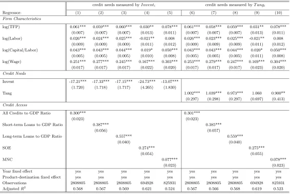
We report our baseline results of equation (11) with the firm-product-country level prices as dependent variable based on four measures of credit needs computed by US data in Tables 3 and 4. In each of
the four sets of results, we use three types of bank loans to GDP ratio and the different types of firm ownership to control for credit access, and employ one of the four measures of financial vulnerability (i.e., external finance dependence, R&D intensity, inventory-to-sales ratio, and asset tangibility) to
proxy for credit needs. Table3presents the results using external finance dependence in specifications (1)-(5) and R&D intensity in specifications (6)-(10). On the other hand, Table 4 reports the results
based on inventory-to-sales ratio in specifications (1)-(5) and asset tangibility in specifications (6)-(10).
In Tables3and4, specifications (1)-(3) and (6)-(8) show the regression results under three different measures of credit access using bank loans. Specifications (4)-(5) and (9)-(10) include two firm-type dummy variables: SOE, which is equal to 1 if the firm belongs to state-owned enterprises (SOE) and
1 and further discussion on measures of credit access in Section 3.3.1, we expect the coefficients on three types of bank loans as well as SOE and MNC to be positive under the endogenous quality
case. We find that the coefficients on all measures of credit access are positive and significant at 1% level, implying that firms with more access to bank loans set higher prices, and the prices set by SOE and MNC are higher than the prices set by DPE and JV, respectively. These results fully
support Proposition1 that tighter credit constraints resulting from lower level of credit access reduce the optimal export price set by a firm, ceteris paribus.
Likewise, if quality is indeed an endogenous choice by the firm, according to Proposition 1 and the further discussion of credit needs measures in Section 3.3.2, we expect the coefficients on external
finance dependence, R&D intensity, and inventory-to-sales ratio to be negative while the coefficients on asset tangibility to be positive. This is because firms in industries with higher external finance
dependence, R&D ratio, and inventory-to-sales ratio face tighter credit constraints whereas those with more tangible assets have more relaxed credit constraints. Again, the results presented in Tables3and
4confirm Proposition 1: ceteris paribus, higher credit needs lowers the optimal prices with statistical significance at 1% level.20
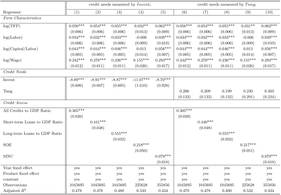
Next, we employ the firm-product level prices (i.e., log price by firmf for producth at year t) as dependent variable and report the results in Tables5 and 6. The results are consistent with those in
Tables3 and 4.
Moreover, Proposition 1 predicts that export prices increase in productivity. The reason is that
firm productivity affects product prices through two channels. On the one hand, higher-productivity firms have lower marginal costs, leading to lower product prices. On the other hand, more productive
firms choose to produce goods of higher quality, leading to higher product prices. As the quality effect dominates, the total effect is that prices increase in productivity. In all specifications of the baseline results in Tables 3-6, the coefficients on TFP are always significantly positive, consistent with the
predictions of the endogenous quality case.
4.1.2 Alternative Specifications
(1) Cross-sectional Estimation
The predictions from our model are cross sectional, i.e., we compare firms facing tighter credit constraints with those who are not. Also the measures of credit constraints only capture the cross-sectional pattern: the industry-level credit needs measures and the regional-level credit access measures
are both persistent and thus averaged over time. Therefore, to fully sort out the time variation effect,
20According to the corporate finance literature, external finance dependence might vary by nature for young firms and
we also estimate one year data (in 2004) using the following equation:
logpricef h(c)=b0+b1log(T F Pf) +γXf +χ1F inDevr+χ2ExtF ini+ϕh(c)+ǫf h(c). (15)
Table 7 reports the cross-sectional results: Columns (1)-(5) report results of equation (15) with country index c and columns (6)-(10) report results without destination country index. The results show that coefficients on credit access are all significantly positive across different specifications and coefficients on external fiance dependence are all significantly negative. This suggests that tighter credit constraints resulting from either lower credit access or higher credit needs indeed reduce export
prices. Also, most coefficients on TFP are still significantly positive, except for SOE in column (4). This is potentially because larger SOE typically employ a lot of unnecessary labor to produce. As a
result, the estimated TFP of SOE may not accurately reflect their productivity.
(2) Different Fixed Effects
As we discussed earlier, the issue of adding different fixed effects terms is not straightforward since
our data contains multiple dimensions and the merging between US data and Chinese data further complicates this issue. Nevertheless, we try different combinations of fixed effects terms with the baseline regressions in Table8. The left panel (columns 1-6) in Table8 report results based on prices
across product-destination and the right panel (columns 7-12) report results of prices across product. In each panel, the first five columns add 2-digit industry fixed effects, and all results regarding the
effects of credit constraints on export prices as well as the relationship between productivity and prices remain similar as in the baseline.
It is more interesting to add firm fixed effects. The last column of each panel in Table 8 adds firm-product-destination (or firm-product) fixed effects in column 6 (or 12) to identify whether the
relationship between credit needs (via external finance dependence) and export prices is operative at the within-firm-product-country (or firm-product) level.21 Such a specification would moreover
provide a more stringent set of controls against the possibility of firm-level omitted variables. Again, the results in columns 6 and 12 confirm the significantly negative coefficients on external finance dependence, indicating that tighter credit constraints resulting from higher credit needs indeed lower
export prices even even at the most disaggregated, within-firm-product-country level. Also the positive relationship between productivity and export prices still holds after adding such fixed effects.
(3) Clustering at Different Level
Another potential issue is a multi-way clustering issue (Cameron et al.,2011) since our data con-tains multiple dimensions and also involves merging between US data and Chinese data. To better
address this clustering issue, we report the results by different clustering in Table 9. We cluster stan-dard errors by 3-digit ISIC in columns 1-5, by province in columns 6-8, by ownership in columns 9-10,
and by product in columns 11-15. We cluster by province and by ownership in some specifications because our credit access measures are computed either by region or by ownership.
When clustering by ISIC or by product, the previous results, such as negative coefficients on external finance dependence, still hold, further confirming that tighter credit constraints resulting
from higher credit needs indeed reduce the optimal price set by exporting firms. When clustering by region, coefficients on total credits to GDP ratio and long-term loans to GDP ratio still remain positive
and significant at 1% level, and the coefficient on short-term loans to GDP ratio is also positive.22 When clustering by ownership, the two coefficients on SOE and MNC are both significantly positive, further confirming that the relationship between credit access and export prices is consistent with
Proposition1.
4.1.3 Results based on Chinese data
As all the above results use the credit needs measures based on US data, to further verify our baseline results, we also compute the key measurement of credit needs—external finance dependence—using
Chinese firm data, and report regression results in Table10. Specifications (1)-(5) of Table10use (log) average export price by firm and HS8-product-destination as dependent variable, while specifications
(6)-(10) use (log) average export price by firm and HS8-product as dependent variable. As discussed in Section 3.3.2, the ranking of industries in external finance dependence calculated based on Chinese data is quite similar to the one based on US data. Thus, as expected, the results based on the external
finance dependence from Chinese data are also consistent with the predictions in Proposition 1: the coefficients on credit access are significantly positive; the coefficients on credit needs are significantly
negative; the coefficients on TFP are significantly positive as well. The results are stated in Table10. To demonstrate robustness, in all subsequent analyses, we run two sets of regressions using external finance dependence computed by US data and Chinese data, respectively.23
4.2 Credit Constraints and Export Quality
If the mechanism of quality adjustment is correct, according to equation (7) and Proposition 2, we expect that given productivity, a firm with more credit access or less credit needs chooses higher
product quality. We now use estimated quality and quality-adjusted price to test this proposition.
Table11replicates the baseline regressions (specifications 1-5 in Table3) by replacing export prices with the estimated product quality as dependent variable in the left panel (columns 1-5). We find
that the coefficients on external finance dependence are negative, and the coefficients on credit access measures are positive. Hence, quality choice is indeed affected by credit constraints. Moreover, the
22Financial development in a region is usually a long-run effect. This potentially could explain why the coefficient on
short-term loans to GDP ratio is not significant when clustering at province level.
23We report the results using the US-based measure of external finance dependence in the main tables, but the results