A Cyclic Cosmological Model Based on the
f
(
ρ
) Modified
Theory of Gravity
Yaoming Shi
University of California, Berkeley, USA1 Email: [email protected]
Received June 6, 2013; revised July 1, 2013; accepted August 3,2013
Copyright © 2013 Yaoming Shi. This is an open access article distributed under the Creative Commons Attribution License, which permits unrestricted use, distribution, and reproduction in any medium, provided the original work is properly cited.
ABSTRACT
We consider FLRW cosmological models for perfect fluid (with ρ as the energy density) in the frame work of the f(ρ) modified theory of gravity [V. N. Tunyak, Russ. Phys. J. 21, 1221 (1978); J. R. Ray, L. L. Smalley, Phys. Rev. D. 26, 2615 (1982)]. This theory, with total Lagrangian R-f(ρ), can be considered as a cousin of the F(R) theory of gravity with total Lagrangian F(R)-ρ. We can pick proper function forms f(ρ) to achieve, as the F(R) theory does, the following 4 specific goals, 1) producing a non-singular cosmological model (Ricci scalar and Ricci tensor curvature are bounded); 2) explaining the cosmic early inflation and late acceleration in a unified fashion; 3) passing the solar system tests; 4) uni- fying the dark matter with dark energy. In addition we also achieve goal number 5) unify the regular matter/energy with dark matter/energy in a seamless fashion. The mathematics is simplified because in the f(ρ) theory the leading terms in Einstein’s equations are linear in second order derivative of metric wrt coordinates but in the F(R) theory the leading terms are linear in fourth order derivative of metric wrt coordinates.
Keywords: Modified Gravity; Dark Energy; Cosmology; Nonsingular; Cosmological Constant
1. Introduction
F R
f
The rapid development of observational cosmology started from 1990s shows that the universe has under- gone two phases of cosmic acceleration. The first one is called cosmic early inflation [1-5] that occurred prior to the radiation domination (see [6-8] for reviews). The second accelerating phase started after the matter domi- nation. The unknown component (dark energy) gave rise to this late time cosmic acceleration [9-28] (see [29-34] for reviews).
Various theories are developed in an effort to explain the cosmic early inflation and late accelerated expansion. The F R
modified theories of gravity (see [35-37] for reviews) have recently [38,39] become one of the leading popular candidates in 1) producing a non-singular cos- mology model
0R2
,
0R R
; 2) uni-
fying the cosmic early inflation and late accelerated ex- pansion in a continuous fashion; 3) passing the solar tests; 4) unifying the dark matter with dark energy.
In this paper we consider cosmological models based on the (less well known)
theories, the theory can also accomplish the same 4 goals. In addition we show that with f
theory we can accomplish goal number 5) unifying the regular matter/energy with dark matter/energy in a seam- less fashion. One added benefit is that the mathematics is simplified in f
theory. This is because the leading terms in Einstein’s equations are linear in
g
in
g
f
f modified theories of gravity for perfect fluid [40,41]. We show that, like the
the theory but are linear in in
f R
f
theories. the
In Section 2, we briefly review the theory. In Section 3, we consider FLRW cosmology and discuss the resulting Friedmann equations in two flavors: one kind is in terms of
ta t a t
, , a p, ,f
and the other kind is in terms of
t
t , t p, ,f
f
. In Section 4, we consider a cyclic cosmological model and go through the checklist to see if we can accomplish 5 goals mentioned in the abstract. In Section 5, we compare theory with
f R theories, Chaplygin gas, NED etc. Section 6 is the conclusion.
f
2. The
Theory of Gravity
1Major ideas of this paper were conceived when Y. Shi was a postdoc
[40,41], the Einstein equations and the energy-momen- tum density tensor, derived from a Hilbert-Einstein like action,
f
g xd41
G c 1 16
S R
, are given by (withunits ):
1 2
R gR 8 T
eff
u u(2.1)
eff
eff
T p
p g
f
(2.2)
where the effective energy density and the effective pres- sure are given by:
eff
(2.3)
p
f
eff
p f 0
(2.4)
In (2.1)-(2.4) , p0 are the energy density and the pressure of the perfect fluid. Throughout this paper, they are always nonnegative. The effective equa- tion of state parameter, weff
, is then given by:
ln
w p f
1 eff
eff
eff
p
f
(2.5)
When we have f
1,
eff
, peff
p , weff
p and (2.2) reduces to the standard expression for perfect fluid. The terms eff
and peff
may be considered as the pressure and energy density for an effective perfect fluid.We would like to emphasize that the gravitational La- grangian, , is the same as in the Einstein’s general relativity. Only the material Lagrangian is generalized from
R
to f
. We would also like to emphasize that the function f in f
theory is an arbitrary func- tion, just like function F in F R
theory.Since there is no detailed derivation of the energy- momentum tensor (2.2)-(2.4) in [40], and the formulas for energy-momentum tensor in [41] are different from (2.2)-(2.4), we follow the standard text book procedure and provide a detailed derivation of the energy-momen- tum tensor (2.2)-(2.4) in Appendix A.
One benefit of using the concept of effective perfect fluid is that all the exact solutions in the literature for perfect fluid with nonzero and independent pressure are solutions of (2.1) and (2.2). For example, if
x
p x
and
are not related by an equation of state and if
x ,p
x ,g
x
, ,
solves the traditional Ein- stein’s equation for perfect fluid, then
eff x peff x
f
g x
is a solution as well. For
given , we can then obtain
x1 eff
f x
1
eff eff
p x p x x f
p x
.
We remark that the conservation of the enegy-mo- mentum becomes:
1
0 0
2 T R Rg
0
0
0 T 0 T
(2.6)
The conventional formula for the conservation of the enegy-momentum becomes the low-energy approxima- tion of (2.6):
(2.7)
0
T p u u pg (2.8)
One consequence of using this effective perfect fluid concept is that the following energy conditions may or may not be satisfied in general.
0,
0eff eff peff
; (2.9) WEC:
0eff peff
; (2.10)
NEC:
0
3 0
eff eff
eff eff
p p
SEC:
; (2.11)
eff peff
DEC:
f
. (2.12)
We remark that energy-momentum conservation in (2.6) is a different concept than various energy condi- tions in (2.9)-(2.12). (2.6) is an equality but (2.9)-(2.12) are inequalities. (2.5) involves covariant-derivative but (2.9)-(2.12) do not.
The criteria for the selection of , in our opinion, is f
when is small. This condition is neces- sary for passing the solar system tests. The cosmologi- cal constant could be included in f
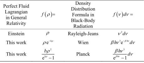
.In Table 1, we present blackbody radiation inspired choices of function f
that, as we show later, can be used to solve the intrinsic singularity problems in GR when goes to infinity and to make the f
theory non-singular.
2
1exp 1
f b b In Table 1, the form
0b1
3
1exp 1
Planck of Table 1 is inspired by the radiation energy density distribution formula,
f d h h d
, that Planck [42,43]
derived in 1901 to solve the ultraviolet diver- gence problem of blackbody radiation. The form
ebf in Table 1 is similar to Wien’s distribu-
tion formula,
d h 3exp
h d
h 1kT
f . In this
Table 1. Comparison of the perfect fluid Lagrangian f(ρ) in General Relativity with the density distribution formula f(v) in black-body radiation (for simplicity, unimportant con- stants are removed in various black-body radiation formu- las).
Perfect Fluid Lagrangian
in General Relativity
f f d
Density Distribution
Formula in Black-Body
Radiation
Einstein Rayleigh-Jeans 2d
This work eb Wien h 3e hd
This work
2
eb 1 b
Planck
3
eh 1
h d
2
1
f d d h kT .
We are amazed, as we show later, that Planck’s magic black-body radiation formula would show its charm again, after over 100 years, in shedding some light on solving the UV divergence problem (intrinsic singularity inside of black hole or at naked singularity, etc.) in Ein- stein’s general relativity theory of gravity as well. Later on we find out that the exponential in
exp
f b or f
b2
exp
b 1
1
1
mf b are not convenient for subsequent mathematical manipu- lation and rational functions like
(m is a positive integer) can do similar job in making
f nonsingular.
From (2.1)-(2.4) we obtain:
2 2
2 2
8 4 3
8 eff 3 eff
R f
p
2p f
2 2
f
(2.13)
2
2 2 2
8 3
8 3 eff eff
R R
f p f
p
(2.14)
So for given p
as long as we pick function
f such that:
lim eff li
m f (2.15)
lim
lim
eff
p
p f
f
R R
(2.16)
We can deduce from (2.13)-(2.14) that 2
0R 0 (2.17) The black-body radiation inspired formulas
exp
f b or f
b2
exp
b 1
1ture tensor nonsingular. If we assume
are clearly satisfying the conditions (2.13)-(2.14) and can be used to make Ricci scalar curvature and the Ricci
curva-
lim p C k
C k, 0
, then we may select
1 m m
nf b
b m, ,n0,mn k
to make R2 and R R nonsingular as well. Equationserve
s (2.15) and (2.16) as one of the sufficient conditions for mak- ing the f
theory of gravity nonsingular.3. The Friedmann Equations
lker (FLRW) cos-
1
2 2 2 2
2 2 2 2 2
1
sin
dt a t k r dr
a t r d d
In Friedmann-Lemaitre-Robertson-Wa
mology, the comoving (infalling) spherical symmetric line element is given by [44]:
2
ds g dx dx
(3.1)
where
a t is the scale factor and t is the cosmolo- e. T
gical tim he energy density
t and pressure p t
are assumed to be functions of well. The Einstein’s equations (2.1) then reduce to the Friedmann equations [40]:
t as
2
2
8 8
3 3
t
eff
a k
f
a
(3.2)
2
4 3
3 8
4 3
t
eff eff
a
p a
f p f
(3.3)
From the conservation of the enegy-momentum
0
T
, one nonzero condition remains [40]:
0 3 t t f
a p
a
(3.4)
Assuming that
0f
only occurs at isolated points, (3.4) then reduces to
0 3
a p
ta t
. (3.5)
Equations (3.3) and (3.5) are not independent; we can pick one and derive the other. Given f
and p
, Equations (3.2) and (3.5) can be use olve th e evolution for the scale factor a t
and energy density d to s e tim
t . Equation (2.5) for weff t
will then tell us effective equation of st
ike at that
what ate looks l
t .We copied Table 2 from [45] to demonstrate what ef-fective equation of state weff
may look like at vari- ous stages of (the las is from [46]). In Figure 1, we will sh w that the effective equation of statet entry o
eff
w for a new cyclic universe model does vary from
−1 to larger than +1 in a continuous fashion. Using (3.5) we obtain
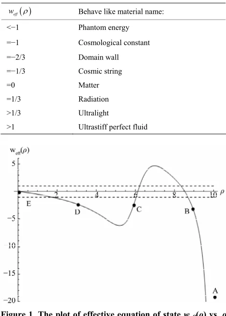
Ta of state weff(ρ) at various values
eff
ble 2. Effective equation of ρ.
w Behave like material name:
<−1 Phantom energy
=−1 Cosmological constant
n
erfect fluid
=−2/3 Domain wall
=−1/3 Cosmic string
=0 Matter
=1/3 Radiatio
>1/3 Ultralight
>1 Ultrastiff p
Figure 1. The plot of effective equation of state weff(ρ) vs. ρ for the M-shaped f(ρ) of (4.1) Numerical constants are l = m = n = 1, p = wρ, w = 0, α = 10, β = 6, γ = 1, λ = 10−3. For con- venience, we also indicate the points A, B, C, D, and E that are shown in Figure 1 and defined in the main text above. The two dashed lines are for weff(ρ) = −1, the phantom cross; and weff(ρ) = +1, the cross over to ultrastiff perfect fluid (see the last entry of Table 2).
3H 3 ta a t p (H t
is Hubble func-
tion) and a
a0exp
1
d p
where a0 of integration. Substituting these results i tois a constant n
(3.2), we can rewrite the Friedmann Equation (3.2) as:
2
2
1 2
0 9
8
exp 2 d
3
t
H p
k
f p
a
2
(3.6)
k0
model, (3.6) reduces to:
For spatially flat
2
8 3
H f
2 2
9
t
p
f and p
. We would prefer to work with Fried- quations the format of (3.6) and (3.7) instead of the Friedman equations in the format of (3.2) and (3.5). This is because, as we show in the next section, that we do not need to specify the Equation of Stateman e in
0p
to obtain major features of cosmology models when
f is given. could bund
We le (3.2) and (3.5) together and write the Friedmann equations in the following different formats as [40]:
(3.7)
This is probably as far as we can go without specifying
2 2
8 3 k
H f
a
(3.8)
3 p H t0 (3.9)
We would consider the Friedmann equations in terms of
ta t a t, , a p, ,f
in terms of
as in (3.8) and (3.9) or
t t , t p, ,f
the major results of the f
as in (3.6)- (3.7) as one of
theory of gravity.This set of Friedmann equations are clearly different from but also closely related to various (modified/gener- alized) Friedmann equations in the literature [47-53]. For example [47] considered a dark fluid with Equation of State like,
p f (3.10) In notation of the current work
tio
, the Einstein’s equa- ns are given by
1
8 G p u u pg (3.11)
The Friedmann equations in this case beco
me,
2 k 8
2 3
H
a
(3.12)
3f H t0 (3.13) We can clearly see that (3.11) and
bu
(3.12) is similar to t different from (3.8) and (3.9).
1) If we identify eff
f
and identify
p peff f p f then (3.12) is t from (3.9). The function
,
identical to (3.8), but (3.13) is differen f and f are related via,
1
f f p f .
2) If we identify , then 3.13) is identical to
(3 erent f
where the Fried- m
( .9), but (3.12) is diff rom (3.8).
Other examples are considered in [48] an equations and Equation of State go like
i1, 2,3
,2 2
8
3 i
i
k H
a
(3.14)
3 0
[image:4.595.57.288.107.421.2] [image:4.595.56.287.109.431.2]
i i i
p p We can that (3.14)-diffe
(3.16) also show (3.16) is similar to but rent from (3.8) and (3.9).
1) If we identify
ii eff
f
and iden- tify
ipi peff
f
p
f
5) is diffe
, then (3.14) is identical to rent from (3.9).
2) If we identify i1
(3.8), but (3.1
, then (3.15) with
i1
isidentical to (3.9), bu s different from (3
4. A Cyclic Cosmological Model
t (3.14) i .8).
flat We now consider a concrete and spatially
k0
el does cosmological model. We will show that our mod
not rely on the signature of the 3D space curvature k to make universe close, open, or flat anymore. The function
f is assumed to be a 7-parameter M-shaped:
22 2
m m
n m
2
1 1
m
n l
m l
f
(4.1)
l m 0
where , ,n0;1n; ; 0. Function f
has two positive roots
,
lex-c
and two comp onjugated roots
m
.1m
im
And f
0 . The constant is selected
f
such that has a local minimum near . Thus f
is M-shaped.This form of f
is the combination of 3 s that of peared in the liteform ten ap rature; namely the RS brane world [54-57]induced form (a) f
1
, the Cardassian expansion [58] form (b)
1 m m
f
0 m 1
, and cosmology con-
f
stant form (c) . The trinsic singularity an
form (a) is used for getting rid of in d producing bounc- ing solution; form (b) and (c) for explaining cosmic late accelerated expansion. We would like to mention that form f
1
was already used in the ori- ginal paper of f
theory of gravity [40] for getting rid of the intrin ity at a t
0 and providing a bouncing solution in the Oppenheimer-Snyder dust collapsing model [59,60].We substitute (4.1) into (3.7) and also rewrite the re- sult in a form mimic 1D Ne
sic singular
wtonian dynamics:
2
1 0
2 t W E (4.2)
2
2
2 2
12
m m
n m
W p
2
1 1
m
n l
m l
(4.3)
Equation (4.2) represents a particle moving in a 1D potential well W
in classic mechanics.We remark that the Firedmann equations expr terms of
essed in
t ,t
t
like those in (4.2) and (4.3) arebetter suited for further discussion and treatment in
f theory than those traditional ones expressed in terms of
a t
,a t
. This is because we do not need to specify function tp
yet in (4.2) and (4.3).As shown in the Figure 2 below that potential well
W is W-shaped (inverse of M-shape because of the negative sign in front of it). Inherited from f
,
W al o h s tw ositive roots s a o p
,
and two complex-conjugated roots
m im
1m
.
0W . This is the reason we would name it
W instead of V
or U
in this paper. Without specifying p
and so Fridmannon (4.2), we can already illu ain fea- lving the
Equati strate the m
model. The big-bang tarts at (Point A)
tures of this cosmological s
[image:5.595.309.539.530.678.2]
t 0 1,t t0 0,W 0
as Figure 2. The top of the m le hump (Point B) isshown idd
near
, the ea osmic inflation happened roughly fromrly c
(Point A) to
1
2
(Point B). The unive the
original FLWR model is roughly between
rse expansion described by
1
2
(Point B) to
(Point C). Weare currently undergoing an accelerated expansion pro- bably in the range from
(Point C) to
1
2
(Point D). The universe will stop expansion at
t T
1, t
t T
0,W 0
c
(Point E)
and turn itself around and start the big crunch and go all the way back to end the big crun h at
t2T ,t t Tthen starts a new big bang
2 0,W 0 (Point A). It —big crunch process. So this cosmological model is a cyclic universe model. This model also covers the eras (like bouncing at both ends which are) beyond the early cosmic inflation and late cosmic accelerated expansion.
Our cyclic universe model with W-shaped potential well do incorporate the cosmic early inflation era as well as the cosmic late accelerated expansion, thanks to two downhill slopes (Point A to Point B and Point C to Point D in Figure 2). This cyclic universe model is thus dif- ferent from those in [61-63] where there is only one downhill slope because their potential U
is a U- shaped.We now define t
24
1 2l2
22
m2 and also consider
as a function of instead of
as a function of . The solution to (4.2) and (4.3) then becomes,
1 1 2
d x p x h x x
(4.4)
2 2
1 n n m m 1 l l
h x x x x x (4.5) The time, T, it takes to go from big-band at Point A to big-stop at Point E is given by:
1 1 2
0 d
T x p x h x x
(4.6) We now assume p
wr
r1
. We empha-size that if 0, then the dominant part tegrand in (4.6) ne
of in
ar x0 becomes x3 2 so (4.6) diverges. t tiny
Thus we need a positive bu (no matter how tiny it is, e.g., 100 m2 in metric unit) to obtain a
T and thus a cyclic universe model. When n 1 10
finite ,
we can relate to the cosmology constant via re of gravita- of lig
cosm nstant
8G
1c4 nstant G d a nega
we nee
(we recove and speed tive but tiny
d the unit ht c ology co
tional co here). Hence
to ology m
1 n r
,
(4 )
al values for
, , , mak In e
A
T finite an ppendix B, we
d the cosm show th
odel cyclic. n l m at wh
, , ,l m n of the e
.4) and (4.5 can be expressed as a linear combination of Elliptical integrals of first kind, third kind, as well as an elementary function arctan. The optim
7-parameters M-shaped f
should be determined by the odel with
ob is is beyond
go thr
als m the a
fitting of this m
servational data. Th our current capability. We now ough our check list to see if we have achieved 5 go entioned in bstract using the cy- clic universe model with 7-paramet M-shaped er f
of (4.1).Goal number (1): producing a non-singular co - logical model
R2
,
0 R R
. rom
cause
t 20 we getsmo F (
0 be
4.2) and (4.3), .
Thus eff
f
is bounded fr m above andbelow in this range. And WEC is also satisfied. To ow o
sh
eff
p is bounded; it is suffice to show that
f
p is bounded. Substituting p = wρr
and (4.1) into
1 r
p f , It is straight forward to show that p
f
is bounded from above and below in the range .ved goal number (
an
Thus via (2.15) and (2.16)
we have achie 1).
Goal number (2): explaining the cosmic early inflation and late acceleration in a unified fashion. See Figure 2
d the description right after.
Goal number (3): passing the solar system tests. As long as , large enough and is tiny enoug have
h, we
f and we can pass the solar system tests. ures 1 and 2 nd the descriptio
number ( : i
r
one material (
Goal number (4): unifying the dark matter with dark
energy. See Fig a n in be-
tween.
l 5) un
Goa fying the regular matter/energy with dark matter/energy in a seamless fashion. Unlike othe dark energy (+ regular matter) theory, there is only
one energy density and one p p) in our
ressure
f theory bas material plays
d in th
wn th
ed cyclic universe model. This single both the role of regular mat- ter/energy when neede e FLRW era and the role of dark matter/energy when needed in other eras in the cy- clic universe model. See Figures 1 and 2 and the de- scription in between for details. It is in this sense that we meant we achieve goal number (5). Maybe regular mat- ter/energy (like perfect fluid) and dark matter/energy are just two aspects of the same material. In other words, we have sho e bright side of the dark matter/energy or the dark side of the regular matter/energy (perfect fluid).
The concept of cyclic universe model itself is not new. For example, any cosmology model in general and cyclic cosmology model in particular, could be reconstructed in
F R theories of gravity. The corresponding technique is described in [64,65]. Realistic F R
gravity cos- mology model has recently been proposed in [66]. This model can a o achieve goals (1) through (4) mentioned above.One unique thing about the f
ls theory based cy- clic model of (4.2) and (4.3) is that, the mathematics is very much simplified. Without specifying p
and solving the Fridmann equations (4.2) and (4.3), we can already il- lustrate the main features of this cosmological model.5. The Relation between
f
(
ρ
) Theory and
F
(
R
) Theories, Chaplygin Gas, NED, etc.
5.1. The Relation between f(ρ) Theory and F(R) Theories
perfect fluid
1 2
8 eff
R
R g R
T T R
F R
(5.1)
perfect fluid
T p uu pg (5.2)
1
8 R
1 16
eff
R
T R
g F R R F R
g g F R
(5.3)
If we equate (2.1) to (5.1), then we obtain a formal re- lation between the energy-momentum tensor of f
ry in (2.2) a
theo nd that of F R
theories in (5.2):
, , 1
p f
perfect fluid , eff
T
T p T F R
F R
(5.4)
It remains to be seen if anything signific
deduced from (5.4). We would look at the relation be- tween f
ant can be
theory and F R
theories (and Palatini
F R theo a different angle. W
looking at thei odified actions against the original Hil- bert-Einstein s first compare the correspond- ing Lagran he corresponding trace equations (with units 8 1 in this section) for dust
ry) from r m action. Let u gians with t
G c
e can start by
(p w , 0) in
We start with (5.5b), the w Table 3 below.
trace of the original Ein- stein’s equation for dust, R. We observe that as long as R and go to infinity at the same speed, the trace equation R can still be satisfied. We that this is the cause of the ic singularity.
think intrins
1) One way to break up this running away (to infinity) situation is to replace R with
exp
R f
b with
1
Planckb .
From
[image:7.595.59.287.626.734.2]this equation, we can immediately obtain R b1. Con- sequently ρis, via R f
exp
b
, also bounded from above and below. If we replace R withTable 3 parison of the angians and trace equa- or f(ρ) theory, F(R) theories, and Palatini
. Com Lagr
tions f F
Rtheory.
Spacetime Lagrangian + Mate angian
Trace of Einstein’s Equation
rial Lagr R T
Hilbert- R R
Einstein −ρ (5.5a) (5.5b) f(ρ) Theory R −f(ρ) (5.6a) R4f 3f (5.6b) f(R) Theo
[68] f(R) (5.7a)
3
2
R R
F R
R F R F R
ry −ρ
(5.7b)
Palatini F(R)
Theory [69] F(R) −ρ (5.8a) R RF R 2F R (5.8b)
1
R f b 2
e can obtain
, w R b1 as well. Of course, we can not just replace with f
in the trace of Einstein’s equations. We h o it at the Lagrangian lev place Lagran- gian of (5.5a) in Einstein’s theory,
ave to d el. Thus we are led to re
R, with that of
f R f
(5.6a) in theory, . The resulting trace equation is (5.6b), R4f
3 f
. Assuming
exp
f b or f
1b
2, straightit is forward to show from (5.6b) that R is bounded from bov a e and below and so is .
2) Anot thi away o in-
fi ation ce Lagrangian o Ein-
stein’s theory,
her way to break up s running (t nity) situ is to repla f (5.5a) in
R, with that of (5.8a) in Palatini
F R theory, F
R . The resulting trace equation is (5.8b), R RF
R 2F
R
. Assuming
exp
2 2
F 1 R with
2
R R lPlanck
, it is straightsh 8b) that 0 1
forward to ow from (5.
bounded from above an tly R , i.e., d below. Consequen is, via R RF
R 2F
R , also bou ed from above and below. If we select F
R Rnd
12R 2
1, we can show that and R are bounded from above and below as well.Because of the higher or ative term in (5.7b), a similar analysis is pr straight for-
der deriv
obably doable but less ward.
y
onlin 72]. A of facto
thors of [40,70] can be tr he fa- mous Born-Infeld theory [
The Lagrangian
5.2. The Relation between f(ρ) Theor and Nonlinear Electro Dynamics (NED)
We are intrigued by the nonsingular exact black hole solutions with N ear Electro Dynamics (NED) [70- s a matter r, the inspiration to both the
original au aced back to t
73].
f and the NED Lagrangian
L F F can be used as material L in the Hilbert-Einstein like action
agrangian
16 1
d4S R f g
x and
1 4
16 d
S
R L F F g x. One major dif- ference between these two theories is that the energy- momentum tensor generated from L F F
is trace-less while as the energy-momentum tensor generated from f
is not.ven by
Recall that in Born-Infeld theory the action is gi
L F j A
d4x
withS
2
1
1 21 det
L F b b F
. The square root
1
4
2
b F F
1 might do a4
L F F F si-
running away situation.
5.3. The Relation between f(ρ y and Chaplygin Gas
74-76]:
sion. Notice that the equation of
milar job in breaking up the
) Theor
The Chaplygin gas is an exotic perfect fluid (a kind of dark energy) with equation of state [
0 , 0 1
p A A (5.9)
It is used to explain the cosmic late accelerated expan- haves like: state be
1 0w p A (5.10)
1
0w p A
2 (5.10)
From Figure 1, we deduce that weff
near
(Point C) ke a Chaplygin gas. The problem with in gas of (5.9) verges at 0behaves li
Chaplyg is that it di-
in the range
0,
. The f
based cyclic universe model of (4.1) does not have kind of divergence problem.
this
6. Conclusions
We considered FLRW cosmological model for perfect fluid (with 0 as the energy density) in the frame work of the f
modified theory of gravity. With antion f
M-shaped func , we achieved, li in ke F R
modified theory of gravity, the following 4 specific goals, 1) producing a non-singular cosmological model
0R2
,
0R R
; 2) explaining the
nd late accelerat
fashion; 3) passing the solar system tests; 4) unifying the dark matter with dark energy.
al numb ifying
the y in a
se
cosmic early inflation a ion in a unified
In addition, we also achieve go er 5) un regular matter/energy with dark matter/energ
amless fashion in f theory and goal number 6) simplifying the Einstein’s equations (in omparison to
cF R theory).
We would like to emphasize that in our f
theory based cyclic universe model, the single material (energy density ) plays bwhen needed in the
oth the regular matter/energy FLRW e he role of dark
e co uid)
same s, we
(per-fect fluid).
(Friedman’s equations) ar
role of
ra and t mat- ter/energy when needed in other eras in the cyclic uni- verse. Thus w njecture that the regular matter/energy (like perfect fl and dark matter/energy might just be two aspects of the material. In other word have probably shown the bright side of the dark matter/ energy or the dark side of the regular matter/energy
The apparent unification of the regular matter/energy with dark matter/energy in a seamless fashion and sim- plification of Einstein’s equations
e probably the two interesting benefits of f
the- ory.7. Acknowledgements
D have
REFERENCES
uring the development of this work, we greatly benefited from the stimulating discussions with Dr. Jie Qing, Dr. J. E. Hearst, Dr. W. M. McClain, Dr. R. A. Harris, Dr. R. P. Lin, Dr. Lei Xu, Dr. Zixiang Zhou, Dr. Ying-Qiu Gu, Dr. Ru-keng Su, Dr. Bin Wang, Dr. Jing- lan Sun, and Dr. W. Liu.
We would also appreciate the feedback from Dr. S. D. Odintsov, Dr. S. Nojiri, Dr. E. Elizalde, Dr. T. P. Sotiriou, Dr. V. Faraoni, and Dr. K. Lake.
[1] A. A. Starobinsky, Physics Letters B, Vol. 91, 1980, pp. 99-102. doi:10.1016/0370-2693(80)90670-X
[2] D. Kazanas, The Astrophysical Journal, Vol. 241, 1980, pp. L59-L63. doi:10.1086/183361
[3] A. H. Guth, Physical Review D, Vol. 23, 1981, pp. 347- D.23.347
356. doi:10.1103/PhysRev
of the Royal Astronomical So- [4] K. Sato, Monthly Notices
ciety, Vol. 195, 1981, pp. 467-479.
[5] G. F. Smoot, C. L. Bennett, A. Kogut, E. L. Wright, J. Aymon, N. W. Boggess, E. S. Cheng, G. de Amici, S. Gulkis, M. G. Hauser, G. Hinshaw, P. D. Jackson, M. Janssen, E. Kaita, T. Kelsall, P. Keegstra, C. Lineweaver, K. Loewenstein, P. Lubin, J. Mather, S. S. Meyer, S. H. Moseley, T. Murdock, L. Rokke, R. F. Silverberg, L. Tenorio, R. Weiss and D. T. Wilkinson, The Astrophysi- cal Journal, Vol. 396, 1992, pp. L1-L5.
doi:10.1086/186504
[6] D. H. Lyth and A. Riotto, Physics Reports, Vol. 314, 1999, pp. 1-14
doi:10.1016/S 6.
0370-1573(98)00128-8.
[7] A. R. Liddle and D. H. Lyth, “Cosmological Inflation and Large-Scale Structure,” Cambridge University Press, Cam- bridge, New York, 2000.
doi:10.1017/CBO9781139175180
[8] B. A. Bassett, S. Tsujikawa and D. Wands, Reviews of Modern Physics, Vol. 78, 2006, pp. 537-589.
doi:10.1103/RevModPhys.78.537
[9] D. Huterer and M. S. Turner,Physical Review D, Vol. 60, 1999, Article ID: 081301.
doi:10.1103/PhysRevD.60.081301
[10] S. Perlmutter, G. Aldering, G. Goldhaber, R. A. Knop, P. Nugent, P. G. Castro, S. Deustua, S. Fabbro, A. Goobar, D. E. Groom, I. M. Hook, A. G. Kim, M. Y. Kim, J. C. Lee, N. J. Nunes, R. Pain, C. R. Pennypacker, R. Quimby, C. Lidman, R. S. Ellis, M. Irwin, R. G. McMahon, P. Ruiz-Lapuente, N. Walton, B. Schaefer, B.
A. Diercks, P. M. Garnavich, R. L. Gilliland, C. J. Hogan,
98, pp. 1009-1038. S. Jha, R. P. Kirshner, B. Leibundgut, M. M. Phillips, D. Reiss, B. P. Schmidt, R. A. Schommer, R. C. Smith, J. Spyromilio, C. Stubbs, N. B. Suntzeff and J. Tonry, The Astrophysical Journal, Vol. 116, 19
doi:10.1086/300499
[12] A. G. Riess, R. P. Kirshner, B. P. Schmidt, S. Jha, P. Challis, P. M. Garnavich, A. A. Esin, C. C
Grashius, R. E. Schild, P. L. Berli
arpenter, R.
ilippenko roner, J. P. Hughes, P. nd, J. P. Huchra, C. F. Prosser, E. E. Falco, P. J. Benson, C. Bricẽno, W. R. Brown, N. Caldwell, I. P. Dell’Antonio, A. V. F
A. A. Goodman, N. A. Grogin, T. G , J. Green, R. A. Jansen, J. T. Kleyna, J. X. Luu, L. M. Macri, B. A. McLeod, K. K. McLeod, B. R. McNamara, B. McLean, A. A. E. Milone, J. J. Mohr, D. Moraru, C. Peng, J. Peters, A. H. Prestwich, K. Z. Stanek, A. Szent- gyorgyi and P. Zhao, The Astrophysical Journal, Vol. 117, 1999, pp. 707-724. doi:10.1086/300738
[13] M. Tegmark, et al. (SDSS Collaboration), Physical Re- view D, Vol. 69, 2004, Article ID: 103501.
doi:10.1103/PhysRevD.69.103501
[14] M. Tegmark, et al. (SDSS Collaboration), Physical Re- view D, Vol. 74, 2006, Article ID: 123507.
doi:10.1103/PhysRevD.74.123507
[15] D. J. Eisenstein, et al. (SDSS Collaboration), The Astro- physical Journal, Vol. 633, 2005, pp. 560-574.
doi:10.1086/466512
[16] W. J. Percival, S. Cole, D. J. Eisenstein, R. C. Nichol, J. A. Peacock, A. C. Pope and A. S. Szalay, Monthly No- tices of the Royal Astronomical Society, Vol. 381, 2007, pp. 1053-1066. doi:10.1111/j.1365-2966.2007.12268.x [17] D. N. Spergel, et al. (WMAP Collaboration), The Astro-
physical Journal Supplement Series, Vol. 148, 2003, pp. 175-194. doi:10.1086/377226
[18] D. N. Spergel, et al. (WMAP Collaboration), The Astro- physical Journal Supplement Series, Vol. 170, 2007, pp. 377-408. doi:10.1086/513700
[19] E. Komatsu, et al. (WMAP Collaboration), The Astro- physical Journal Supplement Series, Vol. 180, 2009, pp. 330-376. doi:10.1088/0067-0049/180/2/330
[20] V. Sahni, Classical and Quantum Gravity, V
pp. 3435-3448. ol. 19, 2002,
DPB Summe
ysic [21] S. E. Deustua, et al., “Cosmological Parameters, Dark En-
ergy and Large Scale Structure,” APS/DPF/ Study on the Future of Particle Physics
r (Snowmass 2001) ed N Graf, eConf C010630 P342, arXiv:astro-ph/0207293v1. [22] M. S. Turner and D. Huterer, Journal of the Ph
ciety of Japan, Vol. 7
al So- 6, 2007, Article ID: 111015. doi:10.1143/JPSJ.76.111015
[23] T. Padmanabhan, Current Science, Vol. 88, 2005, p. 1057. [24] M. Ishak, Foundations of Physics, Vol. 37, 2007, pp. 1470-
1498. doi:10.1007/s10701-007-9175-z
[25] M. Szydlowski, JCAP, Vol. 0709, 2007, p. 007.
[26] E. V. Linder, Journal of Physics A, Vol. 40, 2007, p. 6697. doi:10.1088/1751-8113/40/25/S14
[27] C. Clarkson, M. Cortes and B. Bassett, JCAP, Vol. 0708, 2007, p. 011.
[28] Y.-Q. Gu, “Dynamic Behavior and Topological Structure of the Universe with Dark Energy,” arXiv:0709.2414v5 [gr-qc].
[29] V. Sahni and A. A. Starobinsky, International Journal of Modern Physics D, Vol. 9, 2000, pp. 373-443.
doi:10.1142/S0218271800000542
[30] S. M. Carroll, Living Reviews in Relativity, Vol. 4, 2001, 1-56.
http://relativity.livingreviews.org/Articles/lrr-2001-1 [31] T. Padmanabhan, Physics Reports, Vol. 380, 2003, pp.
235-320. doi:10.1016/S0370-1573(03)00120-0
[32] P. J. E. Peebles and B. Ratra, Reviews of Modern Physics, Vol. 75, 2003, pp. 559-606.
doi:10.1103/RevModPhys.75.559
[33] E. J. Copeland, M. Sami and S. Tsujikawa, International Journal of Modern Physics D, Vol. 15, 2006, pp. 1753-1935. doi:10.1142/S021827180600942X
[34] L. Amendola and S. Tsujikawa, “Dark Energy: Theory and Observations,” Cambridge University Press, Cam- bridge, New York, 2010.
doi:10.1017/CBO9780511750823
03/RevModPhys.82.451
[35] T. P. Sotiriou and V. Faraoni, Reviews of Modern Physics, Vol. 82, 2010, pp. 451-497.
doi:10.11
Vol. [36] A. De Felice and S. Shinji Tsujikawa, Living Reviews in
Relativity, Vol. 13, 2010, p. 3.
[37] S. Nojiri and S. D. Odintsov, Physics Reports, Vol. 505, 2011, pp. 59-144.
[38] S. Nojiri and S. D. Odintsov, Academic Journal, 1241, 2010, p. 1094.
[39] S. Capozziello, M. De Laurentis, S. Nojiri and S. D. Odintsov, Physical Review D, Vol. 79, 2009, Article ID: 124007. doi:10.1103/PhysRevD.79.124007
[40] V. N. Tunyak, Russian Physics Journal, Vol. 21, 1978, pp. 1221-1223.
[41] J. R. Ray and L. L. Smalley, Physical Review D, Vol. 26, 1982, pp. 2615-2618. doi:10.1103/PhysRevD.26.2615 [42] M. Planck, Annalen der Physik, Vol. 4, 1901, pp. 553-563.
doi:10.1002/andp.19013090310 [43] L. D. Landau and E. M. L
John Wiley, New York, 1972.
ifshitz, “Statistical Mechanics,”
Theory of Relativity,” John
:10.1119/1.2830536 [44] S. Weinberg, “Gravitation and Cosmology: Principles and
Applications of the General Wiley, New York, 1972.
[45] R. J. Nemiroff and B. Patla, American Journal of Physics, Vol. 76, 2008, pp. 265-276. doi
ol. 313, 2012, pp. 385-403.
Modern Physics, Vol. 4, 2007, pp.
2006, Article [46] J. M. Heinzle and P. Sandin, Communications in Mathe-
matical Physics, V
[47] S. Nojiri and S. D. Odintsov, International Journal of Geometric Methods in
115-146.
[48] S. Capozziello, V. F. Cardone, E. Elizalde, S. Nojiri and S. D. Odintsov, Physical Review D, Vol. 73,
ID: 043512. doi:10.1103/PhysRevD.73.043512
2005, Article ID: 023003. doi:10.1103/PhysRevD.72.023003
[50] K. Lake, Physical Review D, Vol. 74, 2006, Article ID: 123505. doi:10.1103/PhysRevD.74.123505
178.
[51] M. Szydlowski, A. Kurek and A. Krawiec, Physics Let- ters B, Vol. 642, 2006, pp.
171-doi:10.1016/j.physletb.2006.09.052
[52] Y. Q. Gu, International Journal of Modern Physics A, Vol. 22, 2007, pp. 4667-4678.
doi:10.1142/S0217751X07037925
[53] Y. Q. Gu, “Accelerating Expansion of the Universe with
etter Nonlinear Spinors,” 2006.
[54] L. Randall and R. Sundrum, Physical Review L s, Vol. 83, 1999, pp. 3370-3373.
doi:10.1103/PhysRevLett.83.3370
[55] L. Randall and R. Sundrum, Physical Review Letters, Vol. 83, 1999, pp. 4690-4693.
doi:10.1103/PhysRevLett.83.4690
[56] Y. V. Shtanov, Reports on Progress in Physics, Vol. 67,
Physics Letters B, Vol. 557, 693(03)00179-5 2004, pp. 2183-2232.
[57] Y. Shtanov and V. Sahni, 2003, pp. 1-6. doi:10.1016/S0370-2
[58] K. Freese and M. Lewis, Physics Letters B, Vol. 540, 2002, pp. 1-8. doi:10.1016/S0370-2693(02)02122-6 [59] J. R. Oppenheimer and H. Snyder, Physical Review, Vol.
56, 1939, pp. 455-459. doi:10.1103/PhysRev.56.455 [60] S. Weinberg, “Gravitation and Cosmology: Principles and
ce, Vol. 296, 2002, pp Applications of the General Theory of Relativity,” John Wiley, New York, 1972.
[61] P. J. Steinhardt and N. Turok, Scien . 1436-1439. doi:10.1126/science.1070462
[62] P. J. Steinhardt and N. Turok, New Astronomy Reviews 1.003
, Vol. 49, 2005, pp. 43-57.
doi:10.1016/j.newar.2005.0
urok, Physical Review .031302
[63] J. Khoury, P. J. Steinhardt and N. T Letters, Vol. 92, 2004, Article ID: 031302. doi:10.1103/PhysRevLett.92
Review D, Vol. 74, [64] S. Nojiri and S. D. Odintsov, Physical
2006, Article ID: 086005. doi:10.1103/PhysRevD.74.086005
[65] S. Nojiri and S. D. Odintsov, Journal of Physics: Confe-
. Odintsov, L. Sebastiani and S. , Article ID:
odern Phys- 0)
. Eq.(8)
ws of Modern Physics, , rence Series, Vol. 66, 2007, Article ID: 012005.
[66] E. Elizalde, S. Nojiri, S. D
Zerbini, Physical Review D, Vol. 83, 2011 086006.
[67] T. P. Sotiriou and V. Faraoni, Reviews of M ics, Vol. 82, 2010, pp. 451-497. Eq.(1
[68] T. P. Sotiriou and V. Faraoni, Reviews of Modern Physics, Vol. 82, 2010, pp. 451-497
[69] T. P. Sotiriou and V. Faraoni, Revie Vol. 82, 2010, pp. 451-497. Eq.(20)
[70] E. Ayon-Beato and A. Garcia, Physics Letters B, Vol. 464 1999, pp. 25-29. doi:10.1016/S0370-2693(99)01038-2 [71] K. A. Bronnikov, Physical Review D, Vol. 63, 2001, Ar-
ticle ID: 044005. doi:10.1103/PhysRevD.63.044005
47504
[72] J. Matyjasek, Physical Review D, Vol. 70, 2004, Article ID: 047504. doi:10.1103/PhysRevD.70.0
, pp. 425-451. [73] M. Born and L. Infeld, Proceedings of the Royal Society
of London. Series A, Vol. 144, 1934 doi:10.1098/rspa.1934.0059
[74] M. C. Bento, O. Bertolami and A. A. Sen, Physical Re- view D, Vol. 66, 2002, Article ID: 043507.
doi:10.1103/PhysRevD.66.043507
[75] A. Y. Kamenshchik, U. Moschella and V. Pasquier, Phy- sics Letters B, Vol. 511, 2001, pp. 265-268.
doi:10.1016/S0370-2693(01)00571-8
[76] M. Chevallier and D. Polarski, International Journal of Modern Physics D, Vol.10, 2001, pp. 213-224.
doi:10.1142/S0218271801000822
[77] S. W. Hawking and G. F. R. Ellis, “Gravitation and Cos-
al Functions,” Science mology: Principles and Applications of the General The- ory of Relativity,” John Wiley, New York, 1972.
[78] Z. X. Wang and D. R. Guo, “Speci