Munich Personal RePEc Archive
Environmental efficiency indices: towards
a new approach to green-growth
accounting
Peroni, Chiara
STATEC
1 February 2012
Environmental efficiency indices:
towards a new approach to green-growth accounting
Chiara Peroni∗
Institute National de la Statistique et des Etudes Economiques, Luxembourg
(Preliminary and incomplete)
May 8, 2012
Abstract
This article analyses the link between environmental and productive efficiency in a group of EU member states and the US using data from the UN Framework Convention on Climate Change. Its main indicator, carbon intensity, is defined as the ratio of total greenhouse gases emissions to output. A non-parametric frontier approach enables mod-elling a multiple output technology in which greenhouse gas emissions are an undesirable outcome of a production process. A DEA method is used to compute environmental ef-ficiency indices, which grade countries according to their ability to increase production while reducing pollutants, under minimal assumptions. The only assumptions are that bad outputs are costly to dispose of and that returns to scale are variable. The study shows that productive efficiency is considerably lowered when environmental degradation are taken into account. Only two (Luxembourg and Sweden) out of 16 countries are envi-ronmentally efficient. Malmquist indices, however, show that environmental performances improved over the period considered in nearly all countries. A decomposition of carbon intensity, which links emission performance to technical progress, is also presented; this highlights the positive contribution of labour productivity on the reduction in carbon intensity. Finally, no evidence of a DEA-based environmental Kuznet curve is found.
KEYWORDS: Carbon intensity; data envelopment analysis; Malmquist index; decom-position; Kuznet curve.
∗Statec & ANEC & Observatoire de la Comp´etitivit´e. Corresponding address: Statec, 13, Rue Erasme,
Environmental protection and sustainability have an immediate economic and financial impact. There is growing widespread concern related to the effect of industrial activities on the environment and to the consequences of climate change on human welfare. Economic growth is perceived to generate environmental degradation. The link between climate change and human activity has been recently established by a comprehensive study conducted by the Berkeley Earth group, which confirms previous studies by the MET office/CRU-UEA and NASA.1 The idea that production processes and economic policies should take into
ac-count sustainability issues is the focus of demand from (and to) policy makers. At the core of environmental policy guidelines of international organisations such as UN and OECD, is the principle of prevention, which states that technology should aim to reduce pollution. In addition, international agreements (the 1997 Kyoto protocol), which set targets to reduce emissions of greenhouse gases, envisage mechanisms to develop markets for tradable emission quotas or permits. One such scheme, the European Union Emissions Trading Scheme, en-ables less polluting companies to sell their surplus of emission allowances to bigger polluters (Directive 2003/87/EC). In this context, it is crucial to measure how production units (firms, industries, countries) are successful in reducing pollutants.
This study is concerned with measuring the environmental efficiency of countries, where environmental efficiency is defined as the ability of producing more while polluting less. In a production-frontier setting, it incorporates pollutants into production technologies as un-desirable outputs, following Fare et al. (1989), and makes two crucial assumptions on the technology: 1) the elimination of bad outputs is costly (weak disposability); 2) returns to scales are variable. This is implemented by Data Envelopment Analysis (DEA — Charnes et al., 1978), which computes environmental efficiency scores by comparing each economic unit to a best practice frontier, identifying those units that produce lower levels of pollutants
and greater amount of desirable productions.
The DEA approach has several advantages: (a) data requirements are mild; (b) there are no assumptions on the functional form of the technology (sauf returns to scale) or on market structure; (b) its benchmarking nature permits flexible application to different prob-lems/aggregation level.
Advantages of DEA-based measures of environmental efficiency on standard economic approaches have already been pointed out in the literature. This framework does not require observations on undesirable outputs’ prices (Fare et al., 1989). As a result, it avoids placing a monetary weight on environmental impacts, which is regarded as highly controversial, and can compute a single aggregate index which does not require weighting of environmental impacts (Tyteca, 1996, 1997). Here, it is argued that DEA-based indicators of environmental performance offer more robust measures of environmental efficiency than standard indicator. The latter often capture economic cycles and changes in the structure of economies rather than genuine improvements in environmental efficiency which, for example, stems from the adoption of greener technologies.
In this light, the goal of this study is to estimate an enhanced measure of carbon intensity for a group of 15 European Countries and the US from 1995 to 2009. The most recent data on greenhouse gases emissions from the United Nations Framework Convention on Climate Change (UNFCC) are used to construct an aggregate environmental efficiency index (EPI) at country level. Malmquist indices based on the EPIs are also computed, capturing how environmental performance evolves over time. This is done under a Variable Returns to Scale
DEA technology (Zhou et al., 2008). The environmental efficiency scores are compared to pure economic efficiency measures to test the existence of Environmental Kuznet Curves (EKCs), a popular — and much questioned — framework to analyse the relation of environmental degradation to economic growth. Furthermore, it is shown that the frontier approach can lead to an alternative green growth accounting framework, which establishes a link between productive efficiency, technical progress and measures of environmental performance. A pre-vious version of the UN dataset was analysed in DiMaria and Ciccone (2008); computations are carried out using SAS routines developed by these authors.
Related studies are those of Zaim and Taskin (2000a), Fare et al. (2004), Zaim and Taskin (2000b), Zhou et al. (2008), and Zhou et al. (2010), which assess eco-environmental perfor-mance at country or regional level. These studies uses economic data from the OECD and energy consumption and emission data from the International Energy Agency (IEA); they differ mainly in sample periods, countries analysed and measures of bad outputs and inputs. Zaim and Taskin (2000a) study environmental performances of the OECD countries from 1980 to 1990. These authors compare indices obtained under weak and strong disposability, with the aim of computing output losses generated by environmental policies constraints. Zaim and Taskin (2000b) use the same measure of environmental efficiency to test for the existence of EKC within a standard regression framework. Fare et al. (2004) compare production of desirable output (GDP) to multiple undesirable outputs (carbon oxide - CO2, nitrous oxide - N2O, and sulfur oxide - SOX) in a group of industrialised countries for 1990. Inputs are energy consumption, capital stock and labour. These authors compute separate indices to quantify by how much it is possible to increase good output given bad output and inputs use, and by how much it is possible to expand bad output while keeping good output and inputs fixed. The ratio of these two quantities gives the environmental efficiency index. Canada, US, Ireland, Greece and Finland are the countries with the lowest scores. These authors find that environmental performance is significantly affected by variation in oil consumption rather than per capita income. Zhou et al. (2008) compares the environmental performances of 8 world regions (OECD, non-OECD Europe, Africa, etc..) for 2002. Input and outputs are, respectively, energy consumption, GDP and CO2 emissions; thus, the corresponding EPI indices amount to an estimate of ratios of the reciprocal of carbon intensity, while taking into account the carbon factor (emissions/energy). Results show that indeed carbon intensity is correlated to environmental performances. Zhou et al. (2010) extends this framework to compute Malmquist indices, which give the evolution of environmental efficiency over time, for a panel of 18 (top emitters) countries from 1995 to 2004. They found that environmental performance improved by 24%, due mainly to technical progress.
1
The environmental efficiency index
The evaluation of countries’ environmental performance uses a framework originally devel-oped by Farrell (1957) for measuring the productive efficiency of economic units. In this framework, production sets and distance functions generalise the idea of production function. Production sets define technology in terms of feasible input/output sets; distance functions measure operating efficiency by comparing observed output to the boundary of the produc-tion set (the frontier). Distance funcproduc-tions offer a mean of comparing different units in terms of their position to the frontier, and to study the evolution of the units’ performance when the structure of technology changes.
Assume that each economic unit — or Decision Making Unit (DMU) — produces a sin-gle output, denoted by y, using a vector of input x ∈ RN
+. 2
Formally, the production possibility set in periodtis as follows:
St={(xt, yt) :xt can produce yt}; (1)
Here, The set S represents all feasible input/output vectors (x, y) such that usingxone can produce y. The boundary of S, the frontier, gives the maximum output obtainable from a given amount of inputs use. DMUs operating on the frontier are said to be efficient because they make full use of the inputs. The output distance function describes all operating DMUs in terms of their relative position to the frontier:
Dt(xt, yt) =inf{θ: (xt,
yt
θ)∈St, θ ≥0}; (2)
Here,D gives the smallest (infimum) of the set of real numbers θ, where θ is such that the input/output combination (xt, yt) belongs to the production possibility set St.3 Dt(xt, yt)
measures the reciprocal of the required expansion in output given inputs xt to attain the
frontier defined bySt. D takes the value of 1 for those DMUs on the frontier and less than 1
for those DMUs below the frontier. Larger values ofD are associated to units closer to the frontier.
The DEA method (Charnes et al., 1978) provides a way of computing distance functions. DEA selects the most efficient unit for each observed combination of input (that is, the unit which produces the highest amount of output), and constructs the frontier by joining the set of points represented by those efficient units. This is done by solving the following linear programming problem (LP):
maxλ,Φ λ0 (3)
s.t. PJj=1xijφj ≤xi0, for every i −PJj=1yjφj+λ0y0 ≤0
Φ, λ≥0
Here, the subscripts iand j index, respectively, inputs and DMUs; Φ is a vector (J x 1) of coefficients for the DMUs; λis a score to be maximized. (The subscript 0 indicates that the problem is solved with respect to a reference DMUs.) Intuitively, the LP problem above seeks the biggest possible expansion of the output of DMU0, while remaining within the feasibility
set. The solution gives a score for each DMU, λ∗
0; the efficiency measure for DMU0 is equal
to the reciprocal of such score: E0 = 1/λ∗0. The DMUs with a score equal to 1 will define the
efficient frontier.4
The method outlined above can be extended to incorporate pollution as an undesirable output of production technologies. Fare et al. (1989) first extended Farrell’s approach to productive efficiency when production yields outputs that are undesirable and others that are not. In this context, efficiency is measured by the amount by which it is possible to increase output and, at the same time, reduce the amount of pollutants at a given level of inputs use. The best practice frontier identifies those units producing the lowest level of pollutants together with the greatest amount of desirable production. According to Fare et al. (1989), an environmental feasible technology set satisfies the following assumptions:
1. if (x, y, u)∈S and 0≤θ≤1then (x, θy, θu)∈S
2. if (x, y, u)∈S and u= 0 then y= 0
(Here, u denotes the undesirable output.) The first assumption, weak disposability, implies that the disposal of undesirable output is costly and that it is not possible to decrease the production of the bad output without decreasing the production of the good output (or de-creasing inputs’ use) (Fare and Grosskopf, 2004; Fare et al., 1994a). The second assumptions, thepollution problem, states that it is not possible to stop production of bad outputs unless production is stopped altogether. Fare et al. (1989) formulate a DEA problem which permits the expansion of output and the simultaneous contraction of undesirable output, within the constraints imposed by inputs’ use and technology, as follows:
maxλ,Φ λ0 (4)
s.t. PJj=1xijφj ≤xi0, for every i −PJj=1yjφj+λ0y0 ≤0 −PJj=1ujφj+λ−
1 0 u0= 0
Φ, λ≥0
(Here, the equality sign in the constraint for the undesirable output guarantees that weak disposability is satisfied.)5
The resulting optimal score give a measure of efficiency that takes into account the presence of environmental constraints and pollution, an environmental performance indicator (EPI). In the spirit of Fare et al. (1989), Zhou et al. (2008) extend the problem of eq. 4 to consider the computation of environmental efficiency scores under different assumptions on returns to scale, namely non-increasing returns to scale (NIRS) and
4The formulation of problem 3, also referred to as the envelopment form, represents the dual of a non-linear
fractional problem. Charnes et al. (1978) shows how the original problem, which minimises a ratio of input on output, can be transformed into a linear score problem. This clarifies the link between the linear program and the measurement of productive efficiency. The score formulation reduces the dimensionality of the problem as the number of constraints is equal toI (number of inputs) rather thanJ(number of DMU). The optimisation problem presented here is an output-oriented version, but it is also possible to formulate the problem as an input-oriented one. In the latter case, we seek the biggest possible reduction in inputs’ use, while keeping output levels constant.
5Alternative formulations of the DEA environmental problem are possible. One can see Fare et al. (1989,
variable returns to scale (VRS). The LP problem under environmental constraint and VRS is as follows:
minλ,Φ λθ0
0 (5)
s.t. −PJj=1xijφj+xi0 ≥0, for every i
PJ
j=1yjφj+θ0y0 ≥0
PJ
j=1ujφj−λ0u0= 0
PJ
j=1φj = 1
Φ≥0
This problem seeks to minimize the ratio of undesirable inputs to desirable output. The constraint that the DMU’s coefficients’ sum should be equal to one imposes VRS on the technology set. (Note that, once again, this is a non-linear problem, for which Zhou et al., 2008, give a linearised formulation.).
The direct approach outlined above allows us to construct an aggregated environmental performance index (EPI) at country level, which grades countries according to their ability to increase output and decrease desirable output. The EPI is computed at any given point in time. The next section considers the measurement of environmental efficiency performances in a dynamic context.
1.1 Malmquist indices of environmental performance
Caves et al. (1982) first proposed the use of the Malmquist index to measure productivity changes. Given two time period tand t+ 1, the Malmquist index of productivity is defined as follows:
Mt,t+1 =
Dt(xt+1 , yt+1
)
Dt(xt, yt)
Dt+1
(xt+1 , yt+1
)
Dt+1(xt, yt)
12
; (6)
The index is given by the ratio of distance functions obtained by comparing output to inputs in time t and time t+ 1 using a given reference technology. (Here, the geometric averages of indices obtained using both St and St+1
production sets avoids the arbitrary choice of a reference technology.) In other words, equation 6 considers how much a unit could produce using the inputs available int+ 1, if it used the technology at time t, and how much a unit could produce using the inputs available int, if it used the technology available int+ 1.6 Fare
et al. (1994b) showed that equation 6 can be decomposed into efficiency gains and technical progress, as follows:
Mt,t+1 = D
t+1
(xt+1 , yt+1
)
Dt(xt, yt)
| {z }
ef f iciency gains
Dt(xt+1 , yt+1
)
Dt+1(xt+1, yt+1)
Dt(xt, yt)
Dt+1(xt, yt)
12
| {z }
technical progress
; (7)
Here, the first term — a ratio of distances to the frontiers in periodtandt+ 1 — represents the pure change in efficiency. The second term, which measures the shifts in the frontier, provides a measure of technical change.7
This is achieved by comparing, for the same level
of inputs (int ort+ 1), the distance functions obtained under the technology in tand t+ 1. (Once again, we have a geometric mean of ratios obtained under the technology in t and
t+ 1.)
The Malmquist index has been widely applied in the analysis of productivity and total factor productivity changes. In this article, Malmquist indices are computed using distance functions obtained from a VRS environmental DEA technology, which replace standard output distance functions. These give changes in environmental performances over time.
2
The data
This analysis uses data on greenhouse gases emissions and on the economic performances of 15 Western European (EU member) countries and the US from 1995 to 2009. (The analysis is restricted to this group of countries for reasons of data availability and reliability.) Employ-ment and GDP data are gathered from Eurostat and Statec. Energy consumption is sourced from the enery and environment database published by Eurostat, with the exception of the US, for which energy consumption comes from EIA (Energy Information Administration).8
Data on carbon dioxide (CO2), nitrous oxide (N2O), and total greenhouse gases (GHGs) emissions are gathered from the United Nations Framework Convention on Climate Change (UNFCC) database. The series range from 1995 to 2009, the last available observation.9
N2O is included because this gas is a major air pollutant.10 (Data on Metan — CH4 — were briefly
analysed in DiMaria and Ciccone, 2008, .) The remaining of this section briefly describes the data and presents some widely used indicators of environmental performance. Summary statistics for the main variables are reported in Table 9 in the Appendix to this article.
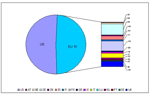
Figure 1 shows that the US were responsible for the largest share of CO2 emissions in 2009, accounting for about the 64% of total CO2 emissions in our sample. Among european countries, the biggest polluters were Germany (about 9% of total emissions), followed by the UK (5.6%), Italy (about 5%), France (4.4%) and Spain (3.5%). All other countries contributed for less than 2% each. Luxembourg emitted the 0.12% of total CO2. (Pie charts for GHGs are not reported, as figure are very close to those in the CO2 graph.) Things look somewhat different when considering shares in N2O emissions, as shown in figure 2. The US and the EU equally shared the N2O emissions; among EU countries, Germany and France were the biggest polluters, with respective shares of 12% and 11%. The UK, Italy, and Spain accounted for, respectively, 6%, 5% and 4.6% of total emissions. Over the period analysed,
8Labour is measured by the domestic employment concept, which includes both resident and non-resident
workers. GDP and employment series are from the Eurostat Economy and Finance database. (The series have been converted using the PPPs, which ensures comparability of aggregates across countries.) Estimates of capital stock are constructed using capital stock data from the EUKLEMS database, downloadable at www.euklems.net, and investment series from Eurostat. Luxembourg data are from the Statec.
9Data are downloadable from the UNFCC website http://unfccc.int/2860.php. The last update of the
database was published in March 2011. Note that the countries considered in our analysis account for a share of 61% of the GHG emissions in the UNFCC database. China and India data are not available in this database.
10While CO2 emissions are the largest contributors to total GHGs emissions, N20 has been found the largest
the US share of emissions increased from 62% recorded in 1995 to the 64% in 2009 for CO2, and from 47% to 51% for N2O.
Figure 1: CO2 emissions for the US and EU in 2009 (% share).(Source: UNFCC).
Figure 2: N2O emissions for the US and EU in 2009 (% share).(Source: UNFCC).
[image:9.612.176.428.367.527.2]Figure 3 presents the countries’ total GHG emissions per worker for selected years. To depict the time series evolution of this indicator, the graph compares beginning-of-period data (1994) to end-of-period data (2009), and includes observations for 2004, the last available year in the study by DiMaria and Ciccone (2008). One can see that, in 1995, the US, Luxembourg and Ireland were the countries with the highest level of emission per capita (> 30 tonnes), followed by Belgium and Finland. The countries’ ranking did not change over the period, but the worst polluters managed to substantially reduce their emissions per capita (with the exception of the US were the decline was moderate). Indeed, the comparison of figures in different years reveals the general fall in GHGs per worker that occurred in nearly all countries. In Greece, Portugal and Austria, emissions recorded in 2004 were higher than in 1995, but fell in 2009 (possibly due to the effect of the financial crisis).
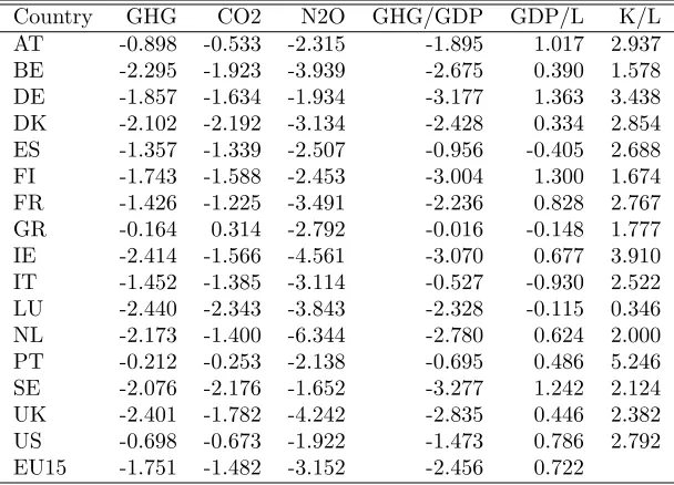
Table 1: Environmental performance indicators: yearly % changes (1995-2009)
Country GHG CO2 N2O GHG/GDP GDP/L K/L
AT -0.898 -0.533 -2.315 -1.895 1.017 2.937 BE -2.295 -1.923 -3.939 -2.675 0.390 1.578 DE -1.857 -1.634 -1.934 -3.177 1.363 3.438 DK -2.102 -2.192 -3.134 -2.428 0.334 2.854 ES -1.357 -1.339 -2.507 -0.956 -0.405 2.688 FI -1.743 -1.588 -2.453 -3.004 1.300 1.674 FR -1.426 -1.225 -3.491 -2.236 0.828 2.767 GR -0.164 0.314 -2.792 -0.016 -0.148 1.777 IE -2.414 -1.566 -4.561 -3.070 0.677 3.910 IT -1.452 -1.385 -3.114 -0.527 -0.930 2.522 LU -2.440 -2.343 -3.843 -2.328 -0.115 0.346 NL -2.173 -1.400 -6.344 -2.780 0.624 2.000 PT -0.212 -0.253 -2.138 -0.695 0.486 5.246 SE -2.076 -2.176 -1.652 -3.277 1.242 2.124 UK -2.401 -1.782 -4.242 -2.835 0.446 2.382 US -0.698 -0.673 -1.922 -1.473 0.786 2.792 EU15 -1.751 -1.482 -3.152 -2.456 0.722
Figure 3: Evolution of GHGs emissions per worker, 1995-2009.(Source: UNFCC, Eurostat).
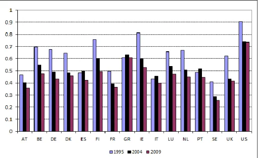
[image:11.612.82.344.425.584.2]Among indicators of environmental performance, carbon intensity is widely used to mon-itor the evolution of emissions at country level (Ang, 1999). Here, carbon intensity is given by total greenhouse gases emissions per unit of GDP. Figure 4 depicts the evolution of this indicator for each country and for selected years. We observe that carbon intensity declined for a large majority of countries. The country ranking, however, is different from the one suggested by the data on emissions per capita. In 1995, the US were the worst performers, followed by Ireland, Finland and Belgium. Luxembourg, the Netherlands, Germany and Den-mark also had high levels of carbon intensity. In 2009 relative positions had changed, with the US still the worst performer but this time round followed by Greece, Ireland, Finland and Belgium and. The downward trend is confirmed by data in Table 1 (fourth column) which show that rates of decrease in carbon intensity were high in a majority of countries over the period, with the exception of Greece.
The figures also suggest some increase in convergence among the countries analysed. (The indicator’s standard deviation drops from 0.14 to 0.10 from 1995 to 2009.) In other words, it seems that countries which experienced the biggest change in carbon intensity were among the worst performers in the beginning of the period, whereas countries with lowest percentage changes in carbon intensity are those comparatively “virtuous” in the beginning of the period. (For example, Belgium is the fourth largest polluter in 1994: its 2009 emissions, however, are about 29% lower than their level in 1994.)
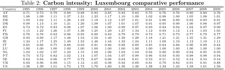
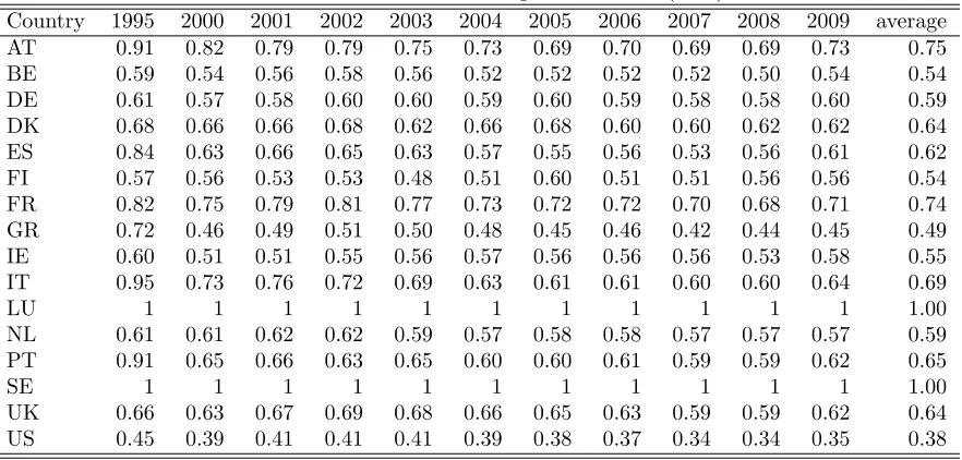
[image:12.612.82.521.509.646.2]To analyse the evolution of countries’ environmental performance with respect to Lux-embourg, the worst EU performers in terms of emissions per capita, table 2 presents carbon intensity series, normalised so that Luxembourg data is equal to 1 in each period. One can see that, overall, Luxembourg was decisively outperformed by several countries, namely Austria, France, Italy, Spain, Sweden and the UK. (These countries have period averages below 1.) Another group of countries, which includes the US, Ireland, Finland and Belgium, performed worse than Luxembourg. Denmark, Germany and the Netherlands data were close to Luxem-bourg. Comparing 2009 to 1995, one observes that the ranking of Luxembourg deteriorated slightly, from the 7t to th 6th position.
Table 2: Carbon intensity: Luxembourg comparative performance
Country 1995 1996 1997 1998 1999 2000 2001 2002 2003 2004 2005 2006 2007 2008 2009 AT 0.71 0.73 0.79 0.89 0.88 0.83 0.85 0.82 0.83 0.75 0.76 0.76 0.80 0.80 0.76 BE 1.06 1.09 1.11 1.37 1.31 1.23 1.17 1.10 1.09 1.02 0.98 1.00 1.05 1.08 1.01 DE 1.03 1.04 1.11 1.26 1.23 1.18 1.12 1.07 1.01 0.91 0.86 0.89 0.92 0.93 0.91 DK 0.99 1.13 1.10 1.21 1.20 1.08 1.07 1.01 1.07 0.91 0.85 0.99 1.00 0.98 0.97 ES 0.74 0.72 0.83 0.98 1.07 1.06 1.00 0.99 0.97 0.93 0.94 0.94 1.02 0.97 0.90 FI 1.15 1.22 1.26 1.37 1.36 1.25 1.29 1.27 1.34 1.12 0.93 1.12 1.14 1.03 1.05 FR 0.76 0.78 0.83 0.98 0.95 0.89 0.83 0.79 0.79 0.73 0.71 0.73 0.77 0.79 0.77 GR 0.93 0.99 1.17 1.48 1.53 1.50 1.40 1.30 1.28 1.18 1.21 1.21 1.35 1.31 1.29 IE 1.24 1.17 1.25 1.49 1.52 1.48 1.44 1.32 1.24 1.11 1.09 1.10 1.12 1.19 1.11 IT 0.65 0.66 0.75 0.88 0.93 0.91 0.86 0.88 0.89 0.85 0.84 0.86 0.90 0.89 0.84 LU 1.00 1.00 1.00 1.00 1.00 1.00 1.00 1.00 1.00 1.00 1.00 1.00 1.00 1.00 1.00 NL 1.02 1.02 1.07 1.22 1.15 1.09 1.06 1.03 1.03 0.94 0.89 0.90 0.94 0.95 0.95 PT 0.74 0.72 0.82 1.02 1.14 1.07 1.04 1.07 0.98 0.96 0.93 0.93 0.98 0.98 0.94 SE 0.62 0.64 0.66 0.77 0.72 0.67 0.66 0.64 0.61 0.53 0.51 0.52 0.54 0.54 0.54 UK 0.94 0.96 0.99 1.15 1.12 1.05 0.98 0.92 0.89 0.81 0.79 0.83 0.91 0.91 0.88 US 1.38 1.39 1.51 1.73 1.73 1.70 1.60 1.56 1.48 1.38 1.34 1.43 1.58 1.61 1.56
The data presented above pose the problem of the relation between common indicators of environmental performance and economic growth, and whether the first are capable of detect-ing genuine improvements in environmental performances. The indicators above are ratios of environmental degradation measures (emissions) to pure economic indicators (employment and output). As a result, an improvement/worsening in one of the measures may reflect economic cycles or changes in the economy’s structure rather than the adoption of environ-mental technologies or increases in energy efficiency. Emissions per capita reflect mainly the evolution in the numerator, whereas carbon intensity figures reflect both changes in output and in emissions.11
Figure 5 presents a scatterplot of rates of growth of GDP per capita versus GHG emissions per capita (growth rates are period averages). One observes several group of countries char-acterised by different relations between income and emissions, thus possible non-linearities in this key relation. The left portion of the graph suggests a positive relation between income and emissions, that is, as the rate of decline in emission lowers, the rate of income growth in-creases. Moving rightwards (lower rates of decline in emissions), the relation income-emissions turns negative. In this region of the graph, increasing emissions are associated to lowering rates of income growth. (Here, we find Austria, the US, Portugal and Greece.) One also observes two possible outliers, Spain (ES) and Italy (IT), characterised by moderate decline in emissions and negative GDP per capita growth.12
Thus, the decline in carbon intensity was the consequence of increases in GDP in Germany, Finland and Sweden, whereas it reflected lower levels of emissions in Luxembourg, Denmark, Belgium and Ireland. In turn, the latter was the likely consequence of the de-indutrialisation process occurring in at least some of those countries (well knwon service-intensive economies). Furthermore, the countries where the decline in carbon intensity was lower are also those countries which experienced low or negative economic growth. (One can see table 1.)
In summary, the descriptive analysis of this section suggests that the relation income-pollution is far from being simple, and that standard indicators may not be adequate in capturing the environmental efficiency of countries. One also notices a contradiction between the general perception of an increase in environmental degradation and reductions in emissions indicators, at least for western European countries and the US. Thus, the remaining of this article attempts to identify better measures of environmental perfromance and review the evidence on their link with economic indicators.
11In western Europe, employment figures were pretty stable in the last decade. One should note, however,
that employment growth was sustained in Ireland and Luxembourg, which may partly explain the decline in emissions per capita in those two countries. On the evolution of inputs and output indicators for the same group of countries analysed in this paper, one can see Peroni (2012).
12A cluster analysis, conducted on several countries characteristics, does not allow to shed further light on
Figure 5: Scatterplot of period average rates of growth of income vs total GHG emissions (per capita). (Source: UNFCC, Eurostat).
3
Eco-environmental performance
This section presents an aggregate environmental performance index (EPI) for the 16 countries in our dataset from 1995 to 2009. This index provides a ranking of countries according to their ability to increase output and decrease the undesirable output. The index implemented here is the mixed environmental performance index (MEI) proposed by Zhou et al. (2008).The underlying environmental DEA technology assumes weak disposability of the undesirable output (Fare et al., 1989) and Variable Returns to Scale (VRS).
Table 3 lists the countries and displays their eco-environmental efficiency scores for selected years from 1995 to 2009. (Full results are reported in the Appendix, Table 10.) The EPIs are obtained by solving the linear programming problem in equation 5 using cross-sectional data. The optimisation problem compares the use of inputs to two categories of output, namely desirable and undesirable output, for each country and for each year. Inputs to production are labour, energy, and capital stock. Output and undesirable output are, respectively, GDP and total greenhouse gases emissions (GHGs). Energy is included as many studies have concluded that this is a relevant input in efficiency analysis (one can see Chen and Yu, 2012, and references therein). The resulting score lie between zero — worst performance — and one — best performance, and their values indicate the factor by which a country can reduce emissions while simultaneously expanding its output and still remain within the feasible production set. For example, a score of 0.35 for the US in 2009 means that this country could expand is production by an amount of 1/0.35 while decreasing by the same amount its emissions.
that is, from an improvement in the technology.
The EPI index is significantly negatively correlated with carbon intensity and emissions per worker indicators, as expected. (An increase in emissions per capita/unit of GDP signals a deterioration in environmental performance.)
[image:15.612.84.525.331.542.2]One also notes that nearly all countries exhibit a deterioration in their performances over the period analysed. (That is, they move further away from the best practise frontier during the period.) The countries experiencing the biggest deterioration are Spain, Italy and Por-tugal. This contrasts the improvements evidenced by standard indicators of environmental performance presented in the previous section, and suggests that it is inappropriate to evaluate environmental performances only by looking at indicators such as carbon intensity or carbon emissions per capita. Efficiency scores, however, are computed using cross-sectional data. Thus, results are better interpreted as static rankings, or cross-sectional measures of perfor-mances. To overcome this limitation and study the evolution of environmental performances over time, the next section presents Malmquist indices of environmental perfromances.
Table 3: Eco-environmental performances (EPI)
Country 1995 2000 2001 2002 2003 2004 2005 2006 2007 2008 2009 average AT 0.91 0.82 0.79 0.79 0.75 0.73 0.69 0.70 0.69 0.69 0.73 0.75 BE 0.59 0.54 0.56 0.58 0.56 0.52 0.52 0.52 0.52 0.50 0.54 0.54 DE 0.61 0.57 0.58 0.60 0.60 0.59 0.60 0.59 0.58 0.58 0.60 0.59 DK 0.68 0.66 0.66 0.68 0.62 0.66 0.68 0.60 0.60 0.62 0.62 0.64 ES 0.84 0.63 0.66 0.65 0.63 0.57 0.55 0.56 0.53 0.56 0.61 0.62 FI 0.57 0.56 0.53 0.53 0.48 0.51 0.60 0.51 0.51 0.56 0.56 0.54 FR 0.82 0.75 0.79 0.81 0.77 0.73 0.72 0.72 0.70 0.68 0.71 0.74 GR 0.72 0.46 0.49 0.51 0.50 0.48 0.45 0.46 0.42 0.44 0.45 0.49 IE 0.60 0.51 0.51 0.55 0.56 0.57 0.56 0.56 0.56 0.53 0.58 0.55 IT 0.95 0.73 0.76 0.72 0.69 0.63 0.61 0.61 0.60 0.60 0.64 0.69
LU 1 1 1 1 1 1 1 1 1 1 1 1.00
NL 0.61 0.61 0.62 0.62 0.59 0.57 0.58 0.58 0.57 0.57 0.57 0.59 PT 0.91 0.65 0.66 0.63 0.65 0.60 0.60 0.61 0.59 0.59 0.62 0.65
SE 1 1 1 1 1 1 1 1 1 1 1 1.00
UK 0.66 0.63 0.67 0.69 0.68 0.66 0.65 0.63 0.59 0.59 0.62 0.64 US 0.45 0.39 0.41 0.41 0.41 0.39 0.38 0.37 0.34 0.34 0.35 0.38
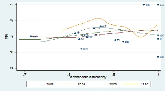
3.1 Is there an efficiency kuznet curve?
performance on productive efficiency scores, are superimposed to the scatterplot to check for the existence of a DEA-based environmental Kuznet curve (EKC).13
[image:16.612.89.369.313.468.2]The curves’ shape evidence inverted U for some years and monotonic relations for others. Clearly, a monotonic relation in this context implies that higher levels of economic efficiencies lead to higher level of environmental efficiencies. An inverted U suggests instead a trade-off, by which, at lower levels of economic efficiency, efficiency gains lead to environmental improvements, whereas at high level of economic efficiency efficiency gains lead to proportional increase in environmental degradation. The inspection of the curves also reveal that the relation between economic and environmental performances is not stable over time. Over the period, the curve becomes lower, meaning that same levels of pure economic efficiency are associated with lower levels of environmental efficiency. In conclusion, an EKC does not seem a stable feature of this data. This simple exercise rather suggests that more research is needed on the relation between environmental and economic performances and a proper account of the time series properties of the data is necessary in order to obtain meaningful results.
Figure 6: Kuznet curves, 1995-2009.(Source: UNFCC, Eurostat).
13Regression curves are obtained with local polynomial fitting, which fits regression lines over portions of
4
Malmquist indices of environmental performance: towards
a new framework for green growth accounting
This section presents Malmquist indices of environmental performance for the 16 countries in the sample. The Malmquist indices allow us to depict the dynamics of the EPI computed in the previous section, and to attribute improvements in environmental performances to increases in efficiency or improvements in technology. Changes in efficiency are usually interpreted as technological catch-up, as they measure how much a country approach the frontier, whereas changes in technology are viewed as the result of innovation efforts (Fare et al., 1994b) or investment in intangibles (Corrado et al., 2009). The indices are computed using equation 6, where distance functions are based on the DEA environmental technology described in Section 1.14 A related study is the one of Zhou et al. (2010), who computed Malmquist indices of total
factor carbon emission performance for the top 18 emitters from 1997 to 2004 using a CRS DEA technology. Here, Malmquist indices are computed under the assumptions of variable returns to scale (VRS), which makes results robust to change in the scale of technology both across countries and over time.
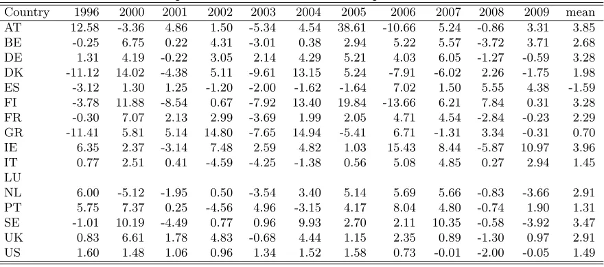
Table 4 presents the estimates of the Malmquist indices of environmental performances for the 16 countries. Table 5 and 6 shows, respectively, the efficiency change and the technological change components (for reasons of spaceonly selected years, ). The last column of each table presents geometric means of yearly changes over the period. The Malmquist index is not available for Luxembourg, due to a feasibility problem. The estimates indicate that all countries, with the exception of Spain, improved their emission performances. A group of countries, comprising Austria, Ireland, Sweden and Germany, was characterised by average growth rates higher than 3%. In some countries the volatility was also high.
One can see that nearly all countries were characterised by efficiency losses. Only Finland, Ireland and the US realised some efficiency gains. Countries which experienced the biggest efficiency losses were Italy, Spain, Portugal and Greece. Sweden and Luxembourg were on the frontier for the entire period. Thus, the improvements in environmental performances were largely driven by technological progress, which was high enough to compensate efficiency losses. One also observes environmental performances deteriorated in the years 2001 and 2008-2009, in correspondence of economic downturns. Once again, it is negative technical changes that drives this results.
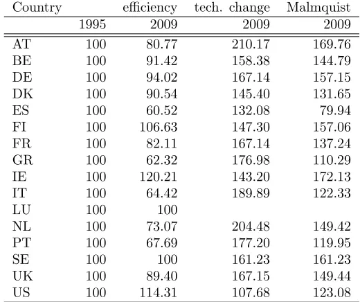
Table 7 shows the cumulative Malmquist index and its component in 2009. (1995 is taken as base year.) This allows to compare relative positions in the end of the period to the base year. Several countries show large improvements, with Ireland, Austria, Sweden, Germany and Finland being the best performers. By contrast, Spain is worse off compared to 1995. Improvements in relative positions in Greece, Italy and Portugal are also modest.
14The computation of the Malmquist index involves the solution of 4 linear programming problems, 2 of
Table 4: Malmquist indices of environmental performance 1995-2009
Country 1996 2000 2001 2002 2003 2004 2005 2006 2007 2008 2009 mean AT 12.58 -3.36 4.86 1.50 -5.34 4.54 38.61 -10.66 5.24 -0.86 3.31 3.85 BE -0.25 6.75 0.22 4.31 -3.01 0.38 2.94 5.22 5.57 -3.72 3.71 2.68 DE 1.31 4.19 -0.22 3.05 2.14 4.29 5.21 4.03 6.05 -1.27 -0.59 3.28 DK -11.12 14.02 -4.38 5.11 -9.61 13.15 5.24 -7.91 -6.02 2.26 -1.75 1.98 ES -3.12 1.30 1.25 -1.20 -2.00 -1.62 -1.64 7.02 1.50 5.55 4.38 -1.59 FI -3.78 11.88 -8.54 0.67 -7.92 13.40 19.84 -13.66 6.21 7.84 0.31 3.28 FR -0.30 7.07 2.13 2.99 -3.69 1.99 2.05 4.71 4.54 -2.84 -0.23 2.29 GR -11.41 5.81 5.14 14.80 -7.65 14.94 -5.41 6.71 -1.31 3.34 -0.31 0.70 IE 6.35 2.37 -3.14 7.48 2.59 4.82 1.03 15.43 8.44 -5.87 10.97 3.96 IT 0.77 2.51 0.41 -4.59 -4.25 -1.38 0.56 5.08 4.85 0.27 2.94 1.45 LU
NL 6.00 -5.12 -1.95 0.50 -3.54 3.40 5.14 5.69 5.66 -0.83 -3.66 2.91 PT 5.75 7.37 0.25 -4.56 4.96 -3.15 4.17 8.04 4.80 -0.74 1.90 1.31 SE -1.01 10.19 -4.49 0.77 0.96 9.93 2.70 2.11 10.35 -0.58 -3.92 3.47 UK 0.83 6.61 1.78 4.83 -0.68 4.44 1.15 2.35 0.89 -1.30 0.97 2.91 US 1.60 1.48 1.06 0.96 1.34 1.52 1.58 0.73 -0.01 -2.00 -0.05 1.49
(Period averages are geometric means of yearly changes. Sources: author’s calculations from UNFCC, Eurostat, Statec data.)
Once again, we find no evidence of environmental Kuznet curves in this data. This time, we compare Malmquist indices of environmental performance to Malmquist indices of pure economic performance and find no clear and stable pattern in the data.
Table 5: Efficiency changes 1995-2009
Country 1996 2000 2001 2002 2003 2004 2005 2006 2007 2008 2009 mean AT 0.25 -18.00 -4.04 0.86 -6.09 -2.12 37.07 -29.59 -2.22 -0.44 6.84 -1.51 BE 0.56 -1.65 3.88 3.49 -3.98 -6.59 -0.13 0.28 -1.64 -2.99 7.44 -0.64 DE 0.52 1.63 -0.63 -21.95 1.12 -2.99 2.02 -1.01 -1.39 -0.62 3.19 -0.44 DK -11.47 6.29 3.39 -12.35 -9.62 33.57 -16.89 -12.93 0.92 2.72 1.19 -0.71 ES 0.00 -6.83 4.82 -2.01 -2.98 -8.49 -4.62 1.83 -5.62 6.25 8.35 -3.52 FI -3.40 1.67 -2.89 -4.93 -4.93 8.49 19.40 -16.70 -0.26 9.28 2.68 0.46 FR -1.08 -1.52 5.72 2.14 -4.65 -5.13 -1.05 -0.37 -2.80 -2.19 3.57 -1.40 GR -26.73 -3.52 14.52 9.97 -1.15 13.27 -42.12 1.14 -8.47 3.78 43.20 -3.32 IE 6.66 -3.90 0.78 9.02 5.08 4.49 -7.45 -1.52 0.07 -5.44 37.05 1.32 IT 0.00 -5.71 3.95 -5.37 -5.20 -8.27 -2.49 -0.02 -2.51 0.94 6.86 -3.09
LU 0 0 0 0 0 0 0 0 0 0 0 0
NL -19.59 -21.85 1.50 -0.33 -4.50 -3.82 1.94 0.56 -1.76 -0.16 0.01 -2.22 PT 5.42 -0.55 7.81 -20.30 4.58 15.95 -21.19 2.31 -2.91 -0.31 5.14 -2.75
SE 0 0 0 0 0 0 0 0 0 0 0 0
UK 0.08 -1.94 5.36 3.96 -1.67 -2.85 -1.92 -2.62 -6.19 -0.65 4.81 -0.80 US 0.80 -1.01 0.64 5.81 5.84 2.95 1.01 -4.13 -4.64 -2.27 -2.91 0.96
[image:19.612.81.559.127.337.2](Period averages are geometric means of yearly changes. Sources: author’s calculations from UNFCC, Eurostat, Statec data.)
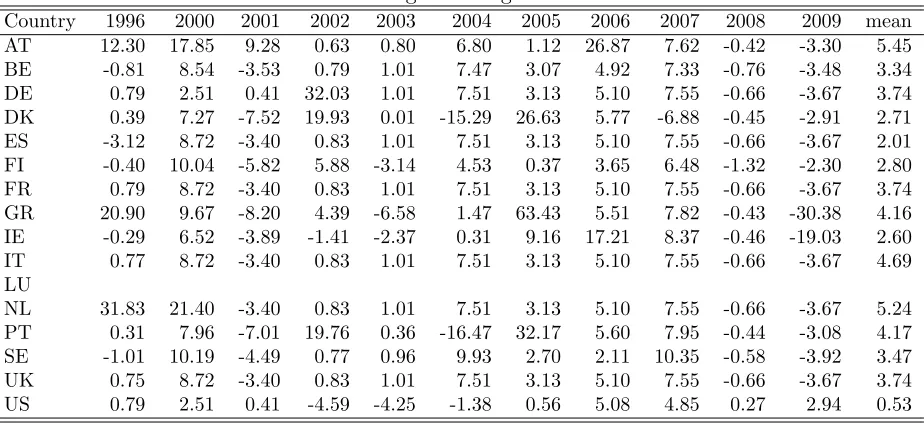
Table 6: Technological changes 1995-2009
Country 1996 2000 2001 2002 2003 2004 2005 2006 2007 2008 2009 mean AT 12.30 17.85 9.28 0.63 0.80 6.80 1.12 26.87 7.62 -0.42 -3.30 5.45 BE -0.81 8.54 -3.53 0.79 1.01 7.47 3.07 4.92 7.33 -0.76 -3.48 3.34 DE 0.79 2.51 0.41 32.03 1.01 7.51 3.13 5.10 7.55 -0.66 -3.67 3.74 DK 0.39 7.27 -7.52 19.93 0.01 -15.29 26.63 5.77 -6.88 -0.45 -2.91 2.71 ES -3.12 8.72 -3.40 0.83 1.01 7.51 3.13 5.10 7.55 -0.66 -3.67 2.01 FI -0.40 10.04 -5.82 5.88 -3.14 4.53 0.37 3.65 6.48 -1.32 -2.30 2.80 FR 0.79 8.72 -3.40 0.83 1.01 7.51 3.13 5.10 7.55 -0.66 -3.67 3.74 GR 20.90 9.67 -8.20 4.39 -6.58 1.47 63.43 5.51 7.82 -0.43 -30.38 4.16 IE -0.29 6.52 -3.89 -1.41 -2.37 0.31 9.16 17.21 8.37 -0.46 -19.03 2.60 IT 0.77 8.72 -3.40 0.83 1.01 7.51 3.13 5.10 7.55 -0.66 -3.67 4.69 LU
NL 31.83 21.40 -3.40 0.83 1.01 7.51 3.13 5.10 7.55 -0.66 -3.67 5.24 PT 0.31 7.96 -7.01 19.76 0.36 -16.47 32.17 5.60 7.95 -0.44 -3.08 4.17 SE -1.01 10.19 -4.49 0.77 0.96 9.93 2.70 2.11 10.35 -0.58 -3.92 3.47 UK 0.75 8.72 -3.40 0.83 1.01 7.51 3.13 5.10 7.55 -0.66 -3.67 3.74 US 0.79 2.51 0.41 -4.59 -4.25 -1.38 0.56 5.08 4.85 0.27 2.94 0.53
[image:19.612.85.547.407.620.2]Table 7: Cumulative changes in eco-environmental performance 1995-2009
Country efficiency tech. change Malmquist
1995 2009 2009 2009
AT 100 80.77 210.17 169.76
BE 100 91.42 158.38 144.79
DE 100 94.02 167.14 157.15
DK 100 90.54 145.40 131.65
ES 100 60.52 132.08 79.94
FI 100 106.63 147.30 157.06
FR 100 82.11 167.14 137.24
GR 100 62.32 176.98 110.29
IE 100 120.21 143.20 172.13
IT 100 64.42 189.89 122.33
LU 100 100
NL 100 73.07 204.48 149.42
PT 100 67.69 177.20 119.95
SE 100 100 161.23 161.23
UK 100 89.40 167.15 149.44
US 100 114.31 107.68 123.08
(Sources: author’s calculations from UNFCC, Eurostat, Statec data.)
4.1 The decomposition of carbon intensity
The EPI index can be interpreted as an enhanced measure of carbon intensity (Zhou et al., 2008). Indeed, these two measures are significantly positively correlated, as noted in previous sections. This section present a decomposition of carbon intensity changes over time using distance functions which provides a link between environmental performance, economic effi-ciency and technical progress. It shows that the change in carbon intensity can be decomposed into the contribution of changes in labour productivity scaled by changes in production and labour input. Labour productivity, in turn, is decomposed in the contribution of capital ac-cumulation, efficiency gains and technical progress (Kumar and Russell, 2002). The following decomposition
The change over time of carbon intensity can be written as the product of changes in the reciprocal of labour productivity and emissions per capita:
CO2t+1/Yt+1 CO2t/Yt
= Yt
Yt+1 Lt
Lt+1 Lt+1
Lt
CO2t+1 CO2t
(8)
=
Yt+1/Lt+1 Yt/Lt
−1
CO2t+1/Lt+1 CO2t/Lt
(This is done by multiplying and dividing carbon intensity by the change in labour input.) Here, CO2 denotes carbon dioxide emissions, Y production, and K and L, respectively, capital stock and labour inputs.
Following Kumar and Russell (2002), we decompose the first term, labour productivity, into the product of changes in efficiency, changes in technology, and (a function of) changes in capital accumulation:
CO2t+1/Yt+1 CO2t/Yt
=
T ECH ×EF F ×f(Kt+1/Lt+1
Kt/Lt
)
−1
CO2t+1/Lt+1 CO2t/Lt
where TECH denotes technical progress, EFF changes in productive efficiency, and f is a function of change in capital intensity.15
One can see that the product of the first two terms in the equation above represent a Malmquist index of production obtained under a CRS technology. Assuming that emissions are an increasing function of production, the change in CO2 per capita can be expressed as the product of the decrease in labour input and an
increasing function of the change in production:16
CO2t+1/Lt+1 CO2t/Lt
= (Lt+1/Lt)−1g(Yt+1/Yt), g′(·)>0, g′′(·)>0 (10)
Thus, the equation 9 for carbon intensity becomes:
CO2t+1/Yt+1 CO2t/Yt
=
T ECH×EF F ×f(Kt+1/Lt+1
Kt/Lt
)
−1
(Lt+1/Lt)−1g(Yt+1/Yt) (11)
Thus, carbon intensity is increasing in production, and decreasing in efficiency gains, techni-cal progress, capital accumulation and labour. Viceversa, carbon efficiency is an increasing function of technical progress, efficiency gains, capital accumulation, employment growth, and a decreasing function of production growth. It is easy to see that technical progress incor-porating newer technologies and new capital, likely to be more energy efficient, can lead to improvements in environmental efficiency. The last two terms are more difficult to interpret. If we assume that output grows at a constant rateα, and that the technology that transforms output in emissions changes over time, we can write the last term as follows:
g(Yt+1/Yt) =g1(Yt+1)/g2(Yt), Yt+1/Yt=α (12)
Rearranging and taking derivatives we get
g1′(Yt)α=g(α)g ′
2(Yt), (13)
Then,
g(α) =αg
′
1(Yt)
g′
2(Yt)
(14)
The expression above offers an interpretation for the last term of equation 11. Asg compares slopes of two functions between two periods, it represents changes in the way that output is transformed into emissions over time. Indeed, one should note that the same level of output can generate different level of emissions depending on the combination of inputs used. For example, it is generally agreed that increases in output lead to increases in pollution through increased energy consumption. Regardless of energy, if a technology implies the use of a bundle of inputs that generates less pollution than other bundles, this should lead to increases in environmental efficiency. (Notice that the decomposition is written in terms of CO2, but is valid also when considering total emissions or any other pollutant in this article.)
15Under CRS and assuming that production is described by a standard Cobb-Douglas function in K and L,
it is possible to show thatf(K/L) = (Kt+1/Lt+1 Kt/Lt )
α.
16g is a positive and increasing function of production. Its second negative with respect to production is
The equation 11 above can be written in terms of distance function as follows:
CO2t+1/Yt+1 CO2t/Yt
= D
t+1
(kt+1 , yt+1
)
Dt(kt, yt)
| {z }
ef f iciency gains
×
Dt(kt+1 , yt+1
)
Dt+1(kt+1, yt+1)
Dt(kt, yt)
Dt+1(kt, yt)
12
| {z }
technical progress
×
Dt(kt, yt)
Dt(kt, yt)
Dt+1
(kt, yt)
Dt+1(kt+1, yt+1)
12
| {z }
capital deepening
×
z(Dt+1
env(xt+1, CO2t+1)/Dtenv(xt, CO2t)) (15)
[image:22.612.100.520.136.253.2]The first three terms, which represents the Kumar and Russell decomposition, are written in terms of standard output distance function, where one output (Y/L=y) is expanded for a given level of the single input (K/L=k). The latter term is left unspecified at this stage. We simply note that it should represent the change in environmental performance for a DEA technology where the objective is to contract the emissions for a certain level of input use. This is interesting because it highlights that the impact of production on CO2 is determined by inputs’ use rather than output itself. (This is also supported by previous study, such as the one of Fare et al., 2004, .)
Table 8 presents figures for carbon intensity and each of its component for the 16 countries from 1995 to 2009. (Data in the table refer to total greenhouse gases emissions.) One can see that, while capital accumulation is sustained and employment grows at positive rates, efficiency gains and technical progress figures are poor. Many countries experience efficiency losses and nearly all of them technical regress.17
(Recall that these terms enter with a minus in the equation for carbon intensity.) Thus, these data suggest that reductions in carbon intensity have been largely driven by improvements in labour productivity, sustained primarily by capital accumulation. This also implies that, had productivity growth being higher, due to efficiency improvements and postive technical progress, the countries performance could have improved even further.18
In summary, the decomposition above establish a link between technical progress, eco-nomic efficiency and environmental efficiency. More research should lead to the complete specification of the decomposition in this section using environmental DEA technologies.
17For a discussion of these results one can see Peroni (2012).
18One should note that figures in the table are period averages, so the decomposition cannot hold exactly.
Table 8: Decomposition of carbon intensity
Country ∆ carbon int. EFF TECH f(∆K/L) ∆L g(∆Y) AT -1.90 0.26 0.35 0.40 0.93 0.12 BE -2.67 -0.16 0.31 0.24 0.99 -1.22 DE -3.18 0.52 -0.23 1.05 0.47 -1.29 DK -2.43 0.07 -1.27 1.54 0.63 -1.36 ES -0.96 -1.13 -0.14 0.81 2.50 1.13 FI -3.00 0.69 -0.17 0.77 1.30 -0.27 FR -2.24 0.08 0.21 0.51 0.90 -0.44 GR -0.02 0.27 -1.65 1.20 1.00 0.92 IE -3.07 -0.21 -1.54 2.44 2.95 0.71 IT -0.53 -1.46 -0.43 0.91 0.92 -0.51 LU -2.33 0.00 -0.15 0.04 3.57 1.27 NL -2.78 0.01 0.08 0.52 1.38 -0.66 PT -0.69 -1.89 -2.64 4.95 0.73 0.53 SE -3.28 1.34 -1.04 0.96 0.57 -1.31 UK -2.84 0.37 -2.19 2.27 0.83 -1.51 US -1.47 0.02 -0.01 0.76 0.78 0.13
Legend: Data are average yearly changes (geometric means). (Sources: UNFCC, Eurostat.)
5
Conclusions
This study investigated the relation between environmental and economic performance for a group of EU member states and the US from 1995 to 2009 using recently published data from the UN Framework Convention on Climate Change. Rather than resorting to standard Environmental Kuznet Curves (EKC), the article models environmental performances using an environmental DEA technology. This regards greenhouse gas emissions as an undesirable output of a productive process, and assumes costly disposability of pollutants. Using this approach, the study computes an environmental performance index (EPI) which allow us to grade countries according to their ability to increase output and decrease emissions at a given level of inputs.
Standard indicators of environmental performances, such as greenhouse gas emissions per capita and carbon intensity, exhibit a substantial decline over the period analysed for nearly all countries, which contrasts with a general perception of improvements in environmental quality in Western countries. The descriptive analysis of the data shows that a non-standard inverse U shaped curve links GDP per capita growth and emissions per capita growth. We find several interesting results:
• Two countries are fully efficient with respect to the EU-US environmental efficiency frontier: Luxembourg and Sweden. Worst performers are US, Greece and Finland. Efficient countries obtain the maximum possible output with the minimum amount of emissions. The simultaneous increase production and decrease emissions can only be achieved through technical progress. In contrast, countries below the frontier can expand their output while reducing pollution.
the environmental constraint. The productive efficiency scores are substantially lowered when greenhouse emissions are taken into account. Furthermore, there is no evidence of a DEA-based EKC in the data.
• Malmquist indices, better suited to describe the time series evolution of efficiency scores than EPIs, evidence a general improvement in environmental performances over the pe-riod. Countries which improved the most were Sweden, Germany, Finland and the Netherlands. These improvements were driven by technical progress. Many countries, however, experienced efficiency losses which determined a poorer environmental perfor-mance.
• A decomposition of carbon intensity using standard output distance functions estab-lishes a positive link between technical progress, economic efficiency gains and carbon intensity. This may explain the findings regarding the EKCs.
The analysis of this article has several limitations. The computation of Malmquist indices under VRS poses problems of feasibility not solvable with standard method available in the literature. This involves a country positioned on the frontier. Moreover, our sample is limited to Western countries, data from developing countries are not considered. The rigorous de-composition of carbon intensity using environmental DEA technology and distance functions requires also further research. The study presented here, however, opens the possibility of a growth accounting exercise that takes into account environmental issues.
References
Ang, B. (1999). Is the energy intensity a less useful indicator than the carbon factor in the study of climate change? Energy Policy, 27:943–946.
Caves, D., Christensen, L., and Diewert, W. (1982). The economic theory of index numbers and the measurement of input, output, and productivity. Econometrica, 50:73–86.
Charnes, A., Cooper, W., and Rhodes, E. (1978). Measuring the efficiency of decision-making units. European Journal of Operational Research, 2:429–444.
Chen, P. and Yu, M. (2012). Total factor productivity growth and directions of technical change bias: evidence from 99 oecd and non-oecd countries. Annals of Operations Research, Online First.
Corrado, C., Hulten, C., and Sichel, D. (2009). Intangible capital and u.s. economic growth.
Review of Income & Wealth, 55:661–685.
DiMaria, C. and Ciccone, J. (2008). Luxklems: Productivite et competitivite. Perpectives de Politique Economique, N 8, Le Gouvernment du Grand-Duche de Luxembourg.
Fare, R. and Grosskopf, S. (2004). Modelling undesirable factors in efficiency valuation: a comment. European Journal of Operational Research, 157:242–245.
Fare, R., Grosskopf, S., and Lovell, C. K. (1994a).Production Frontiers. Cambridge University Press.
Fare, R., Grosskopf, S., Norris, M., and Zhongyang, Z. (1994b). Productivity growth, technical progress and efficiency change in industrialised countries. American Economic Review, 84:666–83.
Fare, R., Grosskopf, S., and Sancho, F. H. (2004). Environmental performance: an index number approach. Resource and Energy economics, 26:343–352.
Farrell, M. (1957). The measurement of productive efficiency. Journal of the Royal Statistical Society, Series A, 120:253–90.
Hua, Z., Bian, Y., and Liang, L. (2007). Eco-efficiency analysis of paper mills along the huai river: An extended DEA approach. Omega, 35:578 – 587.
Kumar, S. and Russell, R. (2002). Technological change, technological catch-up, and capital deepening: relative contributions to growth and convergence. The American Economic Review, 92:527–48.
Peroni, C. (2012). Productivity and competitiveness in luxemnbourg; productivity & the crisis. Perpectives de Politique Economique, N 18, Ministre de l’economie e du commerce exterieur du Grand-Duch de Luxembourg.
Ravishankara, A., Daniel, J., and Portmann, R. (2009). Nitrous oxide (n2o): The dominant ozone-depleting substance emitted in the 21st century. Science, 326:123–125.
Tyteca, D. (1996). On the measurement of the environmental performance of firms. Journal of environmental management, 46:281–308.
Tyteca, D. (1997). Linear programming models for the measurement of environmental per-formance of firms — concepts and empirical results. Journal of Productivity Analysis, 8:183–197.
Zaim, O. and Taskin, F. (2000a). Environmental efficiency in carbon dioxide emissions in the oecd: a non-parametric approach. Journal of Environmental Management, 58:95–107.
Zaim, O. and Taskin, F. (2000b). A kuznets curve in environmental efficiency: an application to OECD countries. Journal of Environmental and Resource Economics, 17:21–36.
Zhou, P., Ang, B., and Poh, K. (2006). Slacks-based efficiency measures for modeling envi-ronmental performance. Ecological Economics, 60:111 – 118.
Zhou, P., Ang, B., and Poh, K. (2008). Measuring environmental performance under different environmental technologies. Energy Economics, 30:1–14.
6
Appendix: tables
Table 9: Summary Statistics: means
Country GDP K L CO2 N2O GHG GDP K GHG CO2 N2O GHG/ nrg nrg/
pc pc pc pc pc GDP GDP
AT 211.13 477.38 37.81 71.11 5.98 85.23 55.71 125.65 22.56 18.81 1.59 0.41 25.28 0.12 BE 254.22 536.58 41.52 122.99 10.06 142.98 61.16 128.87 34.58 29.72 2.44 0.57 36.53 0.14 DE 1996.62 4234.50 389.98 885.64 68.48 1036.95 51.13 108.29 26.63 22.74 1.76 0.53 224.00 0.11 DK 137.39 264.71 27.71 58.50 7.31 72.42 49.55 95.22 26.21 21.18 2.65 0.53 15.18 0.11 ES 801.52 1909.25 172.61 310.28 29.27 380.21 46.62 109.33 22.14 18.02 1.73 0.47 83.51 0.10 EU15 8956.04 0.00 1698.64 3369.63 329.71 4127.15 52.62 24.38 19.88 1.96 0.47 975.38 0.11 FI 123.74 254.15 23.14 61.93 6.53 74.20 53.22 109.33 32.18 26.85 2.83 0.61 24.84 0.20 FR 1387.95 2860.13 254.52 409.20 76.01 565.68 54.41 111.81 22.29 16.11 3.01 0.41 155.78 0.11 GR 194.69 394.26 44.13 103.57 8.29 125.20 44.08 88.91 28.39 23.46 1.89 0.64 19.35 0.10 IE 104.82 167.77 17.49 43.60 8.40 65.94 59.85 94.12 38.38 25.19 4.99 0.64 10.96 0.10 IT 1286.99 2448.47 235.78 464.15 36.48 547.66 54.69 103.38 23.27 19.72 1.56 0.43 125.19 0.10 LU 21.79 73.25 2.82 10.03 0.48 11.02 76.97 258.87 39.35 35.78 1.73 0.51 3.78 0.18 NL 417.28 901.65 81.04 173.99 16.23 214.66 51.38 110.73 26.64 21.54 2.03 0.52 50.67 0.12 PT 162.98 306.76 49.80 60.63 5.39 78.76 32.70 61.15 15.80 12.16 1.09 0.48 17.40 0.11 SE 226.05 405.65 43.13 54.82 7.60 69.66 52.28 93.79 16.20 12.75 1.77 0.31 34.11 0.15 UK 1400.67 2158.00 278.40 547.35 43.73 666.38 50.22 77.18 24.03 19.71 1.58 0.48 148.80 0.11 US 8974.29 15135.45 1390.49 5838.01 320.48 6945.69 64.41 108.30 50.00 42.02 2.31 0.78 2449.83 0.27
Sample 1870.35 2033.00 341.81 740.32 57.67 894.69 53.46 111.56 27.82 22.68 2.17 0.49 288.03 0.13
[image:26.612.80.522.413.548.2]Legend: nrg denotes energy consumption. Units: Greenhouse gases emissions are in billion tonnes of CO2 equivalent (1000 gigagrams - Gg); energy consumption is recorded in million tonnes of oil equivalent (TOE); GDP and capital stock data are in billion euros and employment in 100.000 units. pc indicates that data are in per capita terms.
Table 10: Eco-environmental performances (EPI) 1995-2009
Country 1995 1996 1997 1998 1999 2000 2001 2002 2003 2004 2005 2006 2007 2008 2009 AT 0.91 0.91 0.86 0.88 0.84 0.82 0.79 0.79 0.75 0.73 0.69 0.70 0.69 0.69 0.73 BE 0.59 0.59 0.60 0.56 0.55 0.54 0.56 0.58 0.56 0.52 0.52 0.52 0.52 0.50 0.54 DE 0.61 0.62 0.60 0.61 0.59 0.57 0.58 0.60 0.60 0.59 0.60 0.59 0.58 0.58 0.60 DK 0.68 0.61 0.64 0.66 0.64 0.66 0.66 0.68 0.62 0.66 0.68 0.60 0.60 0.62 0.62 ES 0.84 0.89 0.80 0.79 0.68 0.63 0.66 0.65 0.63 0.57 0.55 0.56 0.53 0.56 0.61 FI 0.57 0.55 0.55 0.57 0.55 0.56 0.53 0.53 0.48 0.51 0.60 0.51 0.51 0.56 0.56 FR 0.82 0.83 0.80 0.79 0.76 0.75 0.79 0.81 0.77 0.73 0.72 0.72 0.70 0.68 0.71 GR 0.72 0.68 0.60 0.53 0.49 0.46 0.49 0.51 0.50 0.48 0.45 0.46 0.42 0.44 0.45 IE 0.60 0.64 0.61 0.56 0.52 0.51 0.51 0.55 0.56 0.57 0.56 0.56 0.56 0.53 0.58 IT 0.95 0.97 0.89 0.87 0.78 0.73 0.76 0.72 0.69 0.63 0.61 0.61 0.60 0.60 0.64
LU 1 1 1 1 1 1 1 1 1 1 1 1 1 1 1
NL 0.61 0.63 0.62 0.63 0.63 0.61 0.62 0.62 0.59 0.57 0.58 0.58 0.57 0.57 0.57 PT 0.91 0.97 0.86 0.78 0.66 0.65 0.66 0.63 0.65 0.60 0.60 0.61 0.59 0.59 0.62
SE 1 1 1 1 1 1 1 1 1 1 1 1 1 1 1
UK 0.66 0.67 0.67 0.67 0.65 0.63 0.67 0.69 0.68 0.66 0.65 0.63 0.59 0.59 0.62 US 0.45 0.46 0.44 0.45 0.42 0.39 0.41 0.41 0.41 0.39 0.38 0.37 0.34 0.34 0.35
Table 11: Economic performances 1995-2009
Country 1995 1996 1997 1998 1999 2000 2001 2002 2003 2004 2005 2006 2007 2008 2009 AT 0.84 0.84 0.84 0.84 0.83 0.85 0.83 0.85 0.85 0.85 0.84 0.88 0.88 0.89 0.87 BE 0.97 0.96 0.97 0.93 0.92 0.95 0.94 0.96 0.94 0.92 0.91 0.93 0.93 0.93 0.92 DE 0.81 0.80 0.78 0.78 0.77 0.77 0.78 0.78 0.78 0.78 0.80 0.85 0.86 0.88 0.84 DK 0.84 0.83 0.82 0.82 0.82 0.83 0.83 0.82 0.82 0.83 0.84 0.85 0.84 0.86 0.86 ES 0.84 0.82 0.80 0.78 0.74 0.73 0.73 0.72 0.71 0.69 0.68 0.68 0.68 0.69 0.71 FI 0.79 0.78 0.79 0.81 0.81 0.83 0.83 0.83 0.83 0.87 0.88 0.91 0.93 0.95 0.90 FR 0.85 0.84 0.85 0.84 0.83 0.84 0.86 0.85 0.82 0.82 0.83 0.85 0.86 0.86 0.86 GR 0.80 0.78 0.77 0.76 0.76 0.76 0.78 0.78 0.79 0.78 0.78 0.79 0.79 0.81 0.83
IE 1 1 1 1 1 1 1 1 1 1 1 1 1 1 1
IT 1.00 0.96 0.94 0.93 0.90 0.89 0.90 0.87 0.85 0.83 0.82 0.83 0.83 0.83 0.81
LU 1 1 1 1 1 1 1 1 1 1 1 1 1 1 1
NL 0.82 0.82 0.81 0.80 0.79 0.80 0.79 0.78 0.76 0.77 0.79 0.81 0.83 0.84 0.82 PT 1 1 0.97 0.93 0.89 0.85 0.82 0.79 0.76 0.75 0.75 0.76 0.77 0.80 0.83 SE 0.80 0.80 0.80 0.82 0.85 0.87 0.87 0.88 0.90 0.94 0.95 0.97 0.98 0.98 0.97
UK 1 1 1 1 1 1 1 1 1 1 1 1 1 1 1
US 1 1 1 1 1 1 1 1 1 1 1 1 1 1 1
[image:26.612.83.518.582.714.2]Table 12: Environmental performances: Malmquist indices 1995-2009
Country 1996 1997 1998 1999 2000 2001 2002 2003 2004 2005 2006 2007 2008 2009 AT 12.58 4.22 5.59 0.85 -3.36 4.86 1.50 -5.34 4.54 38.61 -10.66 5.24 -0.86 3.31 BE -0.25 10.48 -3.33 9.58 6.75 0.22 4.31 -3.01 0.38 2.94 5.22 5.57 -3.72 3.71 DE 1.31 5.99 4.41 7.82 4.19 -0.22 3.05 2.14 4.29 5.21 4.03 6.05 -1.27 -0.59 DK -11.12 17.39 8.79 8.12 14.02 -4.38 5.11 -9.61 13.15 5.24 -7.91 -6.02 2.26 -1.75 ES -3.12 -7.15 -9.18 -14.93 1.30 1.25 -1.20 -2.00 -1.62 -1.64 7.02 1.50 5.55 4.38 FI -3.78 9.20 9.25 6.98 11.88 -8.54 0.67 -7.92 13.40 19.84 -13.66 6.21 7.84 0.31 FR -0.30 5.25 1.38 7.68 7.07 2.13 2.99 -3.69 1.99 2.05 4.71 4.54 -2.84 -0.23 GR -11.41 -4.91 -8.92 3.34 5.81 5.14 14.80 -7.65 14.94 -5.41 6.71 -1.31 3.34 -0.31 IE 6.35 4.74 -0.73 2.83 2.37 -3.14 7.48 2.59 4.82 1.03 15.43 8.44 -5.87 10.97 IT 0.77 6.35 7.43 0.18 2.51 0.41 -4.59 -4.25 -1.38 0.56 5.08 4.85 0.27 2.94 LU